Tests in a Case-Control Design Including Relatives

(1)

Tests in a Case-Control Design Including Rela- tives

STEFANIE BIEDERMANN and EVA NAGEL Department of Mathematics

Ruhr-University Bochum

AXEL MUNK and HAJO HOLZMANN Department of Mathematics

Georg-August-University G¨ottingen ANSGAR STELAND

Department of Mathematics Ruhr-University Bochum

Running Heading: Case-control studies with relatives Abstract

We present a new approach to handle dependencies within the general framework of case-control designs, illustrating our approach by a particular application from the field of genetic epidemiology. The method is derived for parent-offspring trios, which will later be relaxed to more general family structures. For applications in genetic epidemiology we consider tests on equality of allele frequencies among cases and controls utilizing well-known risk measures to test for independence of phenotype and genotype at the observed locus. These test statistics are derived as functions of the entries in the associated contingency table containing the numbers of the alleles under consideration in the case and the control group. We find the joint asymptotic distribution of these entries, which enables us to derive critical values for any test constructed on this basis. A simulation study reveals the finite sample behavior of our test statistics.

Key words: association tests, contingency tables, dependent data, risk measures

(2)

1 Introduction

The aim of this article is to give a new approach to handle data of relatives within a case-control study. We first introduce our method for the situation of parent-child trios with no missing observations, and show later in the discussion how to modify the tests for more general data situations such as more complex pedigrees and missing data. Our approach is based on commonly tests to analyze contingency tables, namely the odds ratio, the attributable risk, and the relative risk. We derive the asymptotic distributions of these test statistics by establishing a general result on the asymptotic normality of the (appropriately standardized) entries of the contingency table. To illustrate our approach we refer to a particular application in genetic epidemiology where the null hypothesis of identical cell probabilities for cases and controls is equivalent to the independence of a specific genotype from the phenotype.

Most methods to detect association with disease in the literature are either pure population based (case-control samples with unrelated individuals only) or pure family based, where parental (founder) genotypes are used to construct tests of association that are entirely contained within the family and thus robust to population stratification. The TDT, for example, which was introduced by Spielman, McGinnis & Ewens (1993), uses nontransmitted parental alleles of a case as a control sample, analyzing the data by a McNemar statistic. Case-control studies, however, tend to have a better power than pure family based procedures;

see, e.g., McGinnis, Shifman & Darvasi (2002). Risch & Teng (1998), Teng &

Risch (1999), and Risch (2000) point out that using pedigrees including many cases will lead to an increase in power, due to higher expected frequencies of disease-susceptibility alleles in pedigrees with multiple cases compared to the frequencies of these alleles in population based cases. Moreover, utilizing all cases in a pedigree rather than just one per pedigree improves power by increasing the effective sample size. Several authors have therefore derived methods to combine the benefits of population based and family based approaches.

(3)

Let us briefly discuss some recent contributions of this kind. Purcell, Sham &

Daly (2005) identify the ignorance of parental phenotypes as one possible source for the lower efficiency of pure family based methods. Fitting a variance component model for nuclear families (both parents and an arbitrary number of children), they break phenotypic association with genotype into two components;

a within component, robust to stratification, in which association is examined within each family, and a between component, where association is examined across families. In their terminology, the TDT consists of a within-family component only, whereas a case-control study with unrelated individuals is entirely a between-family test. Risch & Teng (1998) propose a method, which is applicable to several different designs including sibships with parents, sibships without parents and unrelated controls, using DNA pooling. In Slager & Schaid (2001) the test for trend in proportions introduced by Armitage (1955) is extended to general family data, whereas B¨ohringer & Steland (2006) provide a very accurate version of the likelihood for parent-offspring duos. Whittemore & Tu (2000) present a class of score statistics accommodating genotypes of both unrelated individuals and families with arbitrary structures. Epstein et al. (2005) discuss the issue of sampling both parental and unrelated controls, modifying the approximate analysis approach of Nagelkerke et al. (2004), who had found under quite restrictive model assumptions that analyzing data from triads and unrelated controls to- gether yields a higher power than separate analyses. The approach of Epstein et al. (2005) allows for more flexibility of modelling allele effects, and less restrictive assumptions are needed, without losing power compared with Nagelkerke et al.

(2004). Browning et al. (2005) account for correlations between individuals in a case-control design by calculating an optimal weight for each individual based on IBD sharing probabilities as in McPeek, Wu & Ober (2004), who introduced these optimal weights in the context of finding the best linear unbiased estimator for allele frequencies of data where the relationships among the sampled individuals are specified by a large, complex pedigree such as in isolated founder populations,

(4)

which makes the use of maximum likelihood estimation impractical.

All the methods discussed above are in fact likelihood ratio tests. Since likelihood approaches require a full specification of the genetic model, we propose nonparametric levelα tests to test for independence of genotype and phenotype.

This article is organized as follows. Section 2 deals with a more detailed discussion of the genetic model under consideration. The main results of our research are then stated in Section 3, where the asymptotic distributions of the test statistics are derived. Section 4 provides various important extensions of our method, e.g., polygenic disorders, different inheritance models or strategies to deal with population stratification. To assess the finite sample behavior of the tests in terms of sample size and power, we conduct a simulation study under various scenarios of practical interest in Section 5. The simulations analyze whether including relatives increases statistical power, and also provide a comparison with the TDT, which has become a kind of “benchmark” test among the family based procedures. The simulations demonstrate on the one hand that including relatives in the study always leads to a significant increase in power, and on the other hand that the nonparametric tests have increased power compared to the TDT for virtually all scenarios under consideration under the assumption of no population stratification. The discussion in Section 6 provides a more detailed insight into the problem of dealing with different family structures and the situation of missing data. The proofs of our results, finally, are deferred to an appendix.

2 Genetic model and assumptions

We assume that there are two biallelic lociL1 andL2, withL1 being the candidate locus where data are observed, whereasL2 denotes the true but unknown causal locus. The goal of the study is to ascertain if there is significant evidence for linkage disequilibrium between L1 andL2 by comparing the allele frequencies of a marker allele at L1 in the case and the control group, respectively. We denote the possible alleles at bothL1 andL2 byA and ¯A, where the causative allele for

(5)

the disease atL2 will be termedAin what follows, whereasAatL1 stands for that allele at the marker locus which is suspected to be associated with the disease.

Using the same notation for the alleles at L1 and L2 does not imply that the alleles at the different loci would consist of the same sequence of nucleotides, but is merely for notational convenience. For simplicity of motivation and derivation of results, we further suppose that the underlying inheritance model is dominant, i.e. for any individual the probability of being affected given there is at least one alleleApresent at locusL2 is equal to the penetrance f with 0< f ≤1, whereas individuals without any alleleA atL2 are affected with probability zero. At first glance it seems that our assumptions concerning the number of candidate and disease loci and the mode of inheritance imposed at this stage are quite restrictive, but we show in Section 4 how to apply our approach to an arbitrary number of markers and predisposing loci as well as different modes of inheritance.

We consider the following study setup. A sample ofn₁ affected children (cases) is randomly collected. Similarly, a random sample of n₂ unaffected children forms the basis of the control group. Denote byn =n₁+n₂ the total number of children at stage 1. There are no degrees of relationship allowed among these children to avoid dependencies within the data at this stage of the experiment. To each child from this basic sample we assign a random variableC_i,i= 1, . . . , n,which counts the number of occurrences of allele A at the candidate locus L1, i.e. C_i = 2, 1 or 0, accordingly. In what follows, we will consider the case that data from family trios, i.e. from the children and their parents are available, bringing the total number of individuals taking part in the study to 3n. The random variables corresponding to parental observations are defined equivalently to the offspring data and denoted by A_i and B_i for the first and second parent of the i^th trio, respectively. From the above study setup, it follows that there are dependencies among the data and, as a further complication, the number of parents belonging to either group is also random.

In what follows, we suppose that the following standard assumptions on the

(6)

various processes involved in inheritance are satisfied.

(A1) The random processes yielding the phenotype given the genotype are independent for different individuals.

(A2) Gamete formation is independent of phenotype.

(A3) Hardy-Weinberg equilibrium holds for each locus.

(A4) Offspring data are randomly sampled from the two groups in the population, and the children in the basic sample are unrelated.

Our interest is on testing whether there is an influence of the observed genotype at locus L1 on the phenotype. We therefore test the null hypothesis H₀ that there is no linkage disequilibrium (LD) between the observed locus L1 and the disease locus L2 against the alternative H₁ of the existence of LD between these two loci. Note that the LD coefficientδ describing the LD between alleles at the two loci L1 and L2 within the population is given by δ = δ_AA = h_AA−p_1Ap_2A, whereh_AA denotes the haplotype frequency of alleles A, Aat the lociL1 and L2, and p_1A, p_2A stand for the allele frequencies of A at L1 and L2, respectively. In terms of the LD coefficient δ, the testing problem is thus given by testing the null hypothesis H₀ : δ = 0 against H₁ : δ >0 or H₁ : δ 6= 0, depending on the experimenter’s preference for either a one- or a two-sided alternative. In order to construct tests for these hypotheses, we reformulate the hypotheses in terms of the allele frequencies of A at L1 in the two respective groups. Letp_v denote the frequency of A at L1 among the affected individuals in the population, and p_w the corresponding term among the unaffected individuals. Then p_v and p_w can be expressed in terms of the model parameters δ,f, p_1A and p_2A by

p_v = p_1A+δ 1−p_2A

p_2A(2−p_2A), p_w =p_1A−δ f(1−p_2A)

1−f p_2A(2−p_2A), (1) where a derivation of formula (1) can be found in the appendix. The hypotheses can thus be reformulated equivalently byH₀ :p_v =p_w =p_1AagainstH₁ :p_v > p_w orH₁ :p_v 6=p_w.

(7)

3 The test statistics and their asymptotic dis- tributions

The null hypothesis H₀ implies that the allele frequency of A at locus L1 is the same among affected and unaffected individuals in the population. It is therefore reasonable to consider test statistics based on differences or ratios of estimators for the allele frequencies p_v and p_w to detect deviations from H₀. We choose as estimators ˆp_v and ˆp_w the empirical counterparts of p_v and p_w in the two respective groups, which can be obtained from the corresponding contingency table with entries N₁, N₂, N₃ and N₄, where N₁ denotes the number of alleles A atL1 among the affected individuals,N₂ is the number of A atL1 among the unaffected individuals, and N₃, N₄ are the corresponding numbers of alleles ¯A at L1. Substituting ˆp_v and ˆp_w in the formulae for the risk measures yields the following test statistics

attributable risk T_n1 = ˆp_v −pˆ_w = N₁

N₁+N₃ − N₂ N₂+N₄, odds ratio T_n2 = pˆ_v(1−pˆ_w)

ˆ

p_w(1−pˆ_v) = N₁N₄ N₂N₃, relative risk T_n3 = pˆ_v

ˆ pw

= N₁(N₂+N₄) N2(N1+N3).

We are now ready to present the main result of this article, which gives the joint asymptotic distribution of the empirical allele frequencies ˆp_v and ˆp_w under the null hypothesis H₀. Since under H₀ we have Var(C₁) = Var(A₁) = Var(B₁) and Cov(C₁, A₁) = Cov(C₁, B₁) the results are given in terms of Var(C₁) and Cov(C₁, A₁) instead of these five different expressions for brevity of notations.

The proof of Theorem 1 is deferred to the appendix.

Theorem 1 Suppose the null hypothesis H₀ is valid, assumptions (A1)-(A4) are satisfied and the ration1/nconverges to a positive constant c∈(0,1)forn→ ∞.

Then the joint asymptotic distribution of pˆ_v and pˆ_w is given by

√n ˆ

p_v −p_1A, pˆ_w−p_1A^T _D

−→ N(0,Σ), (2)

(8)

where the entries of the covariance matrix Σ are given by Σ_1,1 = Var(C₁)

12t1

+ c p₁Cov(C₁, A₁)

9t²₁ , Σ_2,2 = Var(C₁)

12 (1−t1) +(1−c)(1−p₂)Cov(C₁, A₁) 9 (1−t1)² , Σ_1,2 = Σ_2,1 = Cov(C1, A1)(c(1−p1) + (1−c)p2)

18t₁(1−t₁)

where p₁ and p₂ denote the probabilities that a parent is affected given the corresponding child is affected or unaffected, respectively. Var(C1) = 2p1A(1−p1A), Cov(C₁, A₁) = p_1A(1−p_1A), and t₁ is the asymptotic expected percentage of affected individuals in the study, i.e. t1 = (c+ 2c p1+ 2(1−c)p2)/3.

Please note that the condition n₁/n → c ∈ (0,1) ensures that the number of data in one of the groups is not outbalanced by the corresponding quantity in the other group. The condition is required in this particular form due to the asymptotic nature of the result of Theorem 1. In a real data application where of course bothn andn₁ are finite, this means that the experimenter should make sure that the ration1/n is not too close to either zero or one to avoid situations where there are almost no cases or no controls in the study.

3.1 Asymptotic distributions of the test statistics

To find asymptotic critical values for the tests under consideration, we utilize the result of Theorem 1 to derive the asymptotic distributions of the test statistics Tn1, log(Tn2) and log(Tn3). Instead of Tn2 and Tn3, we will use the logarithms of these test statistics in the ensuing derivations since log(T_n2) and log(T_n3) were found to preserve the nominal significance level α more precisely in simulations than the original versions of the tests.

Corollary 1 Under the assumptions of Theorem 1 the asymptotic distributions of the test statistics T_n1, log(T_n2) and log(T_n3) under H₀ are given by

√n Tn1

−→ ND (0, σ₁²), √

n log(Tn2)−→ N^D (0, σ²₂), √

n log(Tn3)−→ N^D (0, σ₃²),

(9)

where the asymptotic variances σ₁², σ²₂ and σ²₃ are obtained as

σ₁² = Var(C₁)

12t₁(1−t₁) +Cov(C₁, A₁)(cp₁−(c+cp₁+ (1−c)p₂)t₁+t²₁) 9t²₁(1−t₁)²

= p_1A(1−p_1A) 18t²₁(1−t1)²

2cp₁+ (3−c)t₁−4t²₁ ,

σ₂² = Var(C₁)

12t1(1−t1)p²_1A(1−p1A)² +Cov(C₁, A₁)(cp₁−(c+cp₁+ (1−c)p₂)t₁+t²₁) 9t²₁(1−t1)²p²_1A(1−p1A)²

= 1

18t²₁(1−t₁)²p_1A(1−p_1A)

2cp₁+ (3−c)t₁−4t²₁ ,

σ₃² = Var(C₁)

12t₁(1−t₁)p²_1A +Cov(C₁, A₁)(cp₁−(c+cp₁+ (1−c)p₂)t₁+t²₁) 9t²₁(1−t₁)²p²_1A

= (1−p_1A) 18t²₁(1−t₁)²p_1A

2cp₁+ (3−c)t₁−4t²₁

The assertions of Corollary 1 follow from Theorem 1 and a straightforward application of the ∆-method; see, e.g., Serfling (1980).

3.2 Estimation of unknown parameters

Since the asymptotic variances of the test statistics depend on the unknown parameters p_1A, p₁ and p₂, these parameters have to be estimated in practice.

By Slutsky’s theorem, the results given in Corollary 1 still hold if σ²₁, σ₂² and σ²₃ are replaced by consistent estimators. Under the null hypothesis H₀, the allele frequency p_1A of A at L1 in the two respective groups and the probabilities p₁ and p₂ of a parent being affected given the corresponding child is affected or unaffected, respectively, can be estimated √

n-consistently by the sample means of the corresponding random variables.

For estimating Var(C₁) and Cov(C₁, A₁), there are several approaches. Firstly, one could simply replace p_1A by its estimator ˆp_1A in the relations Var(C₁) = 2p_1A(1−p_1A) and Cov(C₁, A₁) = p_1A(1−p_1A). Alternatively, one could use the estimators ˆv for Var(C₁) and ˆcov for Cov(C₁, A₁) given by

ˆ v = 1

3n

n

X

i=1

(C_i²+A²_i +B_i²)− 1 9n(n−1)

n

X

i=1 n

X

j6=i

(C_i+A_i+B_i)(C_j +A_j+B_j)

(10)

ˆ

cov = 1 2n

n

X

i=1

(C_iA_i+C_iB_i)− 1 9n(n−1)

n

X

i=1 n

X

j6=i

(C_i+A_i+B_i)(C_j +A_j+B_j).

Straightforward calculations show that these estimators are unbiased with variance converging to 0 at a rate of 1/n.

4 Extensions

We demonstrate our method for the case of a monogenic disease and a single marker locus for the sake of clearness and brevity of this article. The proposed tests, however, can readily be extended to genetically more complex models. If a set of k ≥ 1 candidate loci has been chosen we can test as follows whether a specific allele combination (genotype), say G = (g₁, . . . , g_k), at these k loci contributes to the phenotype expression. We define a virtual biallelic locus L with alleles Gand ¯Gwhere ¯G consists of all allele combinations specified by the k markers except the candidate genotype G. The proposed tests can then be applied toLwhere the candidate allele Afrom the original test is replaced by G.

Some slight changes have to be accounted for in the calculation of the variances of the test statistics. In this way, all different allele combinations can be tested with an appropriately corrected significance levelα, which can, e.g., be found by Bonferroni correction or more sophisticated (more powerful) techniques such as Holm’s (1979) or Hochberg’s (1988) procedures or modifications of these. This approach will provide us with p-values for forward and backward selection procedures with respect to single allele combinations and/or marker loci. If the k markers are closely located on the same chromosome one could also think of con- ducting test procedures on haplotypes since classical genetics has demonstrated that the phenotypic effect of several mutations at different loci can sensitively depend on whether the mutations occur in cis or in trans position; see, e.g., Schaid et al. (2002). Again, we can test if a specific haplotype, say H, has an influence on the phenotype by defining a virtual biallelic locus with alleles H and ¯H and

(11)

applying our method. To identify the unknown phase the method of molecular haplotyping can be used if the DNA sequence containing the markers is not too long; see Michalatos-Beloin et al. (1996). Otherwise haplotypes can either be determined by pedigree analysis or haplotype frequencies can be estimated for example by an EM-algorithm; see, e.g., Fallin et al. (2001). A more detailed exploration of this issue will be the subject of further research.

In the situation of a highly inhomogeneous population some care is needed when collecting the data to avoid possible biases of the tests created by population stratification, which is a potential worry in case-control studies; see, e.g., Thomas &

Witte (2002). The simplest ways to cope with this situation would be to include only individuals of homogeneous ethnic and geographic origin, or to categorize the data into the different subpopulations, which are then analyzed separately.

In case of almost equal allele frequencies at the predisposing locus (percentages of affected individuals in each subpopulation are about equal), it is also feasible to

“match” the controls from the basic sample to the cases such that the percentages of different subpopulations are equal in both groups. This will then on average also be true for the parents in the two groups, so that the percentages of different subpopulations will be about equal among the affected and the unaffected individuals. A different strategy to robustify the tests against stratification bias would be to modify the test statistics by estimating p_v and p_w for all subpopulations separately and defining ˆp_v, ˆp_w as the sums (or weighted sums) of the respective estimates. The tests can then be carried out on these modified estimators as before, taking into account the changes in the asymptotic variances. All the methods proposed above, however, rely on knowing the strata, i.e. categoriz- ing individuals into the wrong ethnic group will lead to biased results. Pritchard, Stephens & Donnelly (2000) developed a Bayesian method for the estimation of ethnic origins using genomic information from polymorphic markers that are not linked with the candidate genes under study. The use of this method (or another genomic adjustment approach) can be a helpful supplement to our tests. The

(12)

issue of population stratification may, however, not be dismissed.

At first glance it seems that the genetic inheritance model plays a crucial role, and the question arises, whether the proposed tests also work if the assumption of a dominant mode of inheritance is violated. An inspection of the proof shows that Theorem 1 remains valid even in this general setting. The underlying mode of inheritance influences the asymptotic null distributions only through the values of the parameters p₁ and p₂. These parameters, however, can be consistently estimated from phenotype data, so that the tests can be applied to data from any type of inheritance model.

5 Simulation Study

To assess the finite sample behavior of our tests, we carried out a simulation study for various parameter settings. We were, firstly, interested in investigating whether the inclusion of parental data yields a substantial gain in power, and, secondly, in comparing our tests with the TDT as an already established method.

Thirdly, we examined the sensitivity of the real significance level with respect to the dependency structure of the data. For brevity, we restricted ourselves to simulate the test H₀ : δ = 0 against the one-sided alternative H₁ : δ > 0, which corresponds to the scenario that the experimenter’s belief is in positive LD between A at L1 and A at L2. To simulate random variables with the same distributions asCi, Ai and Bi, i = 1, . . . , n,four parameters have to be specified in advance. In the study at hand we fixed the values of the two allele frequencies p1A,p2A, the penetrancef and the LD coefficientδ. Due to the dependency of the LD coefficientδon the haplotype frequency and the allele frequencies, it is difficult to compare the amount of LD between different pairs of loci using the respective LD coefficients. We therefore use an appropriately standardized version, i.e.

Lewontin’sD⁰ =|δ|/δmax whereδmaxis defined by min{p1A(1−p2A),(1−p1A)p2A} if δ > 0, and δ_max = min{p_1Ap_2A,(1−p_1A)(1−p_2A)} if δ < 0; see, e.g., Devlin

& Risch (1995). In what follows, the parameters will be given in terms of D⁰

(13)

instead ofδ for comparability.

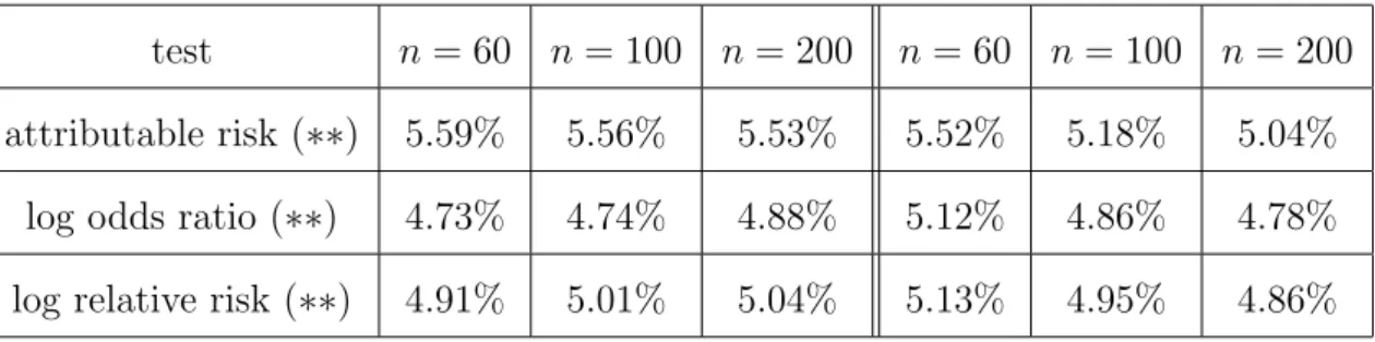
Using a nominal type I error of α = 0.05 we report the empirical rejection rate based on 10,000 runs. Unkown parameters are estimated as explained in Subsec- tion 3.2. We used the sample sizes n = 60, n = 100 and n = 200 for the basic sample, respectively, and the value of n₁ was chosen according to the ”expected equal allocation rule”, i.e. the expected number of affected individuals in the en- tire sample is equal to the expected number of unaffected individuals. For some parameter combinations, this choice was not admissible due to the restriction that n₁ < n. In these situations, we simulated the tests for several choices of n₁ with 0.75n ≤ n₁ ≤ 0.95n, and found that the tests are not very sensitive with respect to the particular choice of n₁ within this range. Table 1 provides results under H₀ : D⁰ = 0 to assess the accuracy of the type I error. Since in what follows we will compare the performance of our tests with the performance of the corresponding tests including either data from unrelated subjects only or data from children with one parent each, we label by (∗∗) the tests including data from both parents for each child.

Table 1 here

It can be seen that our tests preserve the α-level quite well, even for the small sample size of n = 60. Only in the situation of a very small (< 0.05) allele frequency p_1A, the tests do not preserve the α-level when the sample size is small. In this scenario, the test based on the attributable risk appears to be most robust among the three tests under consideration. Our theoretical results provide an explanation for this fact. Indeed, noting that the variances have the formσ²₁ =p_1A(1−p_1A)×f(p₁, p₂) (attr. risk) andσ₂² = 1/{p_1A(1−p_1A)}×f(p₁, p₂) (odds ratio), where f(p1, p2) is a term depending on p1 and p2 only, we see that σ₂² is more sensitive for such p_1A. Increasing the sample size, however, leads to reliable results for all three tests.

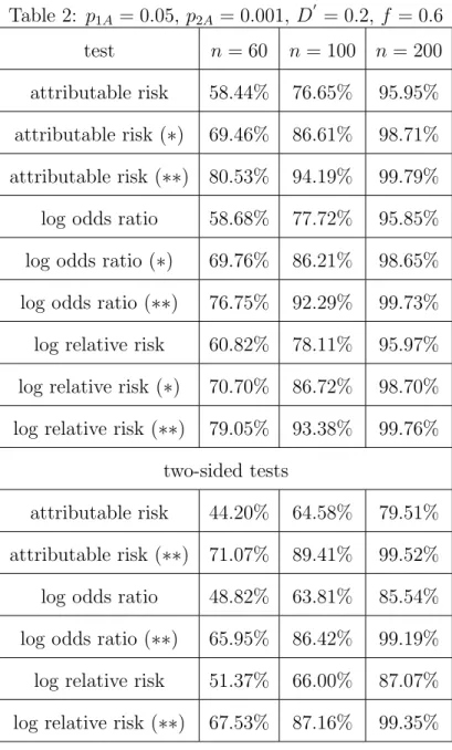
Tables 2, 3 and 4 show the simulated powers of the tests on trios under the alternative hypothesis H1. For comparison, we also display the corresponding

(14)

values when only data of unrelated subjects are included in the test statistics. In this case, the number of affected individualsn₁ was chosen according to the equal allocation rule n₁ =n/2. The tests including offspring data only, thus having a total sample size of n individuals, are not given any label. The tests labeled by (∗) denote the tests including the data from the basic sample plus the data from one randomly chosen parent for each child, bringing the total sample size in this situation to 2n. For these tests, the expected equal allocation rule was used to determine n₁. In Table 2, we chose relatively small allele frequencies of A at the two loci L1 and L2, a small amount of LD measured by D⁰ = 0.2 and a high penetrance of f = 0.6.

Table 2 here

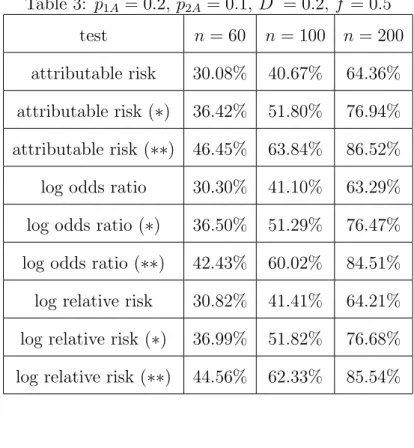
We observe that the inclusion of parental data increases the powers of the tests considerably. We further added the powers of the two-sided tests (H1 : δ6= 0) to Table 2 (scenarios: children only (no label) and both parents included (∗∗)) to show that also in this testing problem the inclusion of parental data significantly increases the capability to detect deviation from H₀. The same holds true for medium scale values of the allele frequencies p1A and p2A as can be seen from Table 3.

Table 3 here

Table 4, finally, displays the values of the simulated powers when the value for the penetrancef is chosen relatively small.

Table 4 here

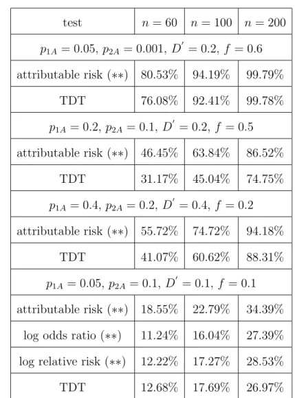
To further assess the practical relevance of a newly developed method it is of great importance to compare its performance with an already established procedure.

We chose the TDT as the competing method in this simulation study since it has become the benchmark method for surveys on trios. Table 5 shows the simulated powers of the TDT for the parameter combinations used above so that they can readily be compared with the powers of the tests (with trios) proposed in this

(15)

article given in Tables 2, 3 and 4. For convenience, the corresponding results for the test based on the attributable risk are given again in Table 5. The number n in this table refers to the number of trios, on which we carried out the tests.

Furthermore, we simulated a scenario where the penetrance f is small (f = 0.1) to assess the power of our tests if the number of affected parents is likely to be small.

Table 5 here

We observe from Table 5 that for all four scenarios our tests perform between

“slightly” better to “significantly” better than the TDT. In particular the test based on the attributable risk has a considerably higher capability to detect deviations from the null hypothesis H0. In the last scenario where p1A is small, we find that the tests based on the relative risk and the odds ratio are less stable than the test based on the attributable risk, which is again due to the form of the asymptotic variances of these tests. In this situation, these two tests are comparable with the TDT.

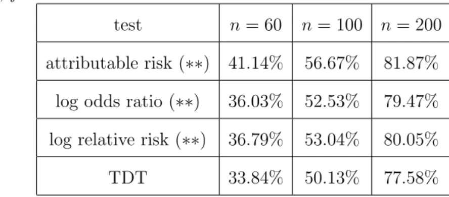
To provide an example for another mode of inheritance than the dominant, we also simulated a recessive inheritance model, and again compared our tests with the TDT. The results, which are very similar to those for the dominant model, are given in Table 6.

Table 6 here

The three tests proposed in this article are asymptotically equivalent, but con- sidering all the tables in this study, we observe that for some scenarios the test based on the attributable risk has a higher power than the other two tests in a finite sample. For many scenarios, however, there is virtually no difference in performance between the three tests. This simulation study therefore indicates that in practice one would best use the test based on the attributable risk, which is also hinted at by further simulation results that are not presented here for brevity.

(16)

6 Discussion

The simulation study reveals that our tests preserve the nominal significance level very well and are quite robust with respect to the genetic parameters. The statistical power to detect linkage disequilibrium, i.e. to detect predisposing genes, is substantially increased by including parental information. Moreover, a comparative power simulation study with respect to the TDT, which has become a benchmark procedure in practical applications, reveals a superiority of our tests (in terms of power) for many scenarios, demonstrating the practical relevance of our approach. These findings are in line with the theoretical results of McGinnis, Shifman & Darvasi (2002) (for unrelated cases and controls), who found that in general fewer case-control samples are required to achieve the same power as the TDT, suggesting greater genotyping efficiency with the case-control design.

The TDT, however, was invented as a test robust to population stratification, which is a potential problem in case-control studies. We have provided some robustification strategies for our tests, which are described in Section 4, but there is no complete solution for this problem. It therefore mainly depends on the structure of the population, which test (our tests or the TDT) might be more appropriate for a particular problem. The reason why our method is more powerful than the TDT seems to be as follows. In contrast to the TDT or other methods based on transmission of marker alleles, we use all available data, i.e. parental phenotypes as well as all parental genotypes, whereas the TDT discards both parental phenotypes and the genotype data of those parents that are homozygote at the observed locus.

The results presented in Section 3 cover the important case that data from parent- offspring trios are available. However, the methodology established in the appendix can be extended to cope with more general family data and the situation of missing data. For example, from a practical viewpoint the generalization to more general types of relatives as the additional inclusion of sibs’ data may be a concern. As an example to get the ideas, we first consider the case where for each

(17)

child from the basic sample the required phenotype and genotype data of both parents and one sib are available. In this scenario, the number of participants in the study is still fixed. From the proof of Theorem 1 in the appendix, we conclude that it is sufficient to extend the random vectorsX_i, i= 1, . . . , n₁, and Y_j, j = 1, . . . , n₂, each corresponding to a child from the two respective groups, by three additional entries giving the phenotype and genotype status of the sib as well as a combination of both exactly analogous to the entries corresponding to the parents. An asymptotic result similar to Lemma 1 can then be proven im- mediately, from which then the asymptotic null distributions of the test statistics can be derived. Other types of relatives can be added to the study analogously, further increasing the sample size and hence the power to detect deviations from the null hypothesis.

Another strategy to increase power would be to sample on the one hand families with many cases and on the other hand unrelated controls, as, under the alternative hypothesis, this will increase the allele frequency difference between the two groups; see, e.g., Risch & Teng (1998), Teng & Risch (1999), and Risch (2000).

It is even possible to allow for missing data under a missing at random assumption. The problem of missing data can be addressed adequately by introducing a random variable indicating if a particular relative takes part in the study or not. Again, the random vectors X_i, i = 1, . . . , n₁, and Y_j, j = 1, . . . , n₂, are extended by these indicators as well as combinations of the indicator variables with random variables giving the genotype and phenotype status of the respective relative. If the study is designed for data from related cases and unrelated controls it is only necessary to modify the vectors X_i, i = 1, . . . , n₁, corresponding to affected children by the indicators. The vectorsY_j, j= 1, . . . , n₂, will then be one-dimensional consisting of the offspring genotype data C_i, i =n₁+ 1, . . . , n.

Note that in these scenarios the number of individuals taking part in the study is random. We therefore have to include the entry N₄ when we calculate the joint asymptotic distribution of the entries of the contingency table since the distribu-

(18)

tion of N₄ is no longer given by the joint distribution of the other entries N₁,N₂ and N₃.

Note that in models extended in such a way additional nuisance parameters describing the dependence structure and the missing data mechanism, respectively, shall appear, and for a practical implementation of the tests the number of parameters to be estimated (complexity of the model), and the increase of data have to be balanced carefully, since estimating too many parameters compared to the increase in available data can lead to poor results. Therefore more detailed investigations of these issues should be a subject of future research.

Acknowledgements

The authors are indebted to two unknown referees, an Associate Editor and the Editor for some really helpful comments, which improved this article and its pre- sentation substantially. This research was supported by the Deutsche Forschungs- gemeinschaft (project: ”Statistical methods for the analysis of association studies in human genetics” and SFB 475 ”Reduction of Complexity for Multivariate Data Structures”). H. Holzmann and A. Munk acknowledge financial support of the Deutsche Forschungsgemeinschaft, MU 1230/8-1. The authors are also grateful to S. B¨ohringer for some interesting discussions and helpful comments on an earlier version of this article.

References

Armitage, P. (1955). Tests for linear trends in proportions and frequencies.

Biometrics 11, 375–386.

B¨ohringer, S. & Steland, A. (2006). Testing genetic causality for binary traits using parent-offspring data. Technical Report. Available at http://www.ruhr- uni-bochum.de/mathematik3/steland.htm#DFG-Project on statistical genetics Browning, S. R., Briley, J. D., Briley, L. P., Chandra, G., Charnecki, J. H.,

Ehm, M. G., Johansson, K. A., Jones, B. J., Karter, A. J., Yarnall, D.

(19)

P. & Wagner, M. J. (2005). Case-control single marker and haplotypic association analysis of pedigree data. Genetic Epidemiology 28, 110–122.

Devlin, B. & Risch, N. (1995). A comparison of linkage disequilibrium measures for fine-scale mapping. Genomics 29(2), 311–22.

Epstein, M. P., Veal, C. D., Trembath, R. C., Barker, J. N. W. N., Li, C. &

Satten, G. A. (2005). Genetic association analysis using data from triads and unrelated subjects. American Journal of Human Genetics76, 592–608.

Fallin, D., Cohen, A., Essioux, L., Chumakov, I., Blumenfeld, M., Cohen, D.

& Schork, N. J. (2001). Genetic analysis of case/control data using estimated haplotype frequencies: Application to APOE locus variation and Alzheimer’s disease. Genome Research11, 143–151.

Hochberg, Y. (1988). A sharper Bonferroni procedure for multiple tests of significance. Biometrika75(4), 800–802.

Holm, S. (1979). A simple sequentially rejective multiple test procedure. Scand.

J. Statist. 6, 65–70.

McGinnis, R., Shifman, S. & Darvasi, A. (2002). Power and Efficiency of the TDT and Case-Control Design for Association Scans. Behavior Genetics 32(2), 135–144.

McPeek, M. S., Wu, X. & Ober, C. (2004). Best linear unbiased allele-frequency estimation in complex pedigrees. Biometrics 60, 359–367.

Michalatos-Beloin, S., Tishkoff, S., Bentley, K., Kidd, K. & Ruano, G. (1996).

Molecular haplotyping of genetic markers 10 kb apart by allele-specific long- range PCR. Nucleic Acids Research24, 4841–4843.

Nagelkerke, N. J., Hoebee, B., Teunis, P. & Kimman, T. G. (2004). Combining the transmission disequilibrium test and case-control methodology using

(20)

generalized logistic regression. European Journal of Human Genetics 12, 964–970.

Pritchard, J. K., Stephens, M. & Donnelly, P. (2000). Inference of population structure using multilocus genotype data. Genetics 155, 945–959.

Purcell, S., Sham, P. & Daly, M. J. (2005). Parental phenotypes in family-based association analysis. American Journal of Human Genetics 76, 249–259.

Risch, N. (2000). Searching for genetic determinants in the new millenium, Nature405, 847–856.

Risch, N. & Teng, J. (1998). The relative power of family-based and case-control designs for linkage disequilibrium studies of complex human diseases. I.

DNA pooling. Genome Research8, 1273–1288.

Schaid, D. J., Rowland, C. M., Tines, D. E., Jacobson, R. M. & Poland, G.

A. (2002). Score tests for association between traits and haplotypes when linkage phase is ambiguous. American Journal of Human Genetics 70, 425–434.

Serfling, R. J. (1980). Approximation Theorems of Mathematical Statistics. Wi- ley, New York.

Slager, S. L. & Schaid, D. J. (2001). Evaluation of candidate genes in case- control studies: a statistical method to account for related subjects. Amer- ican Journal of Human Genetics68, 1457–1462.

Spielman, R. S., McGinnis, R. E. & Ewens, W. J. (1993). Transmission test for linkage disequilibrium: the insulin gene region and insulin-dependent diabetes mellitus (IDDM). American Journal of Human Genetics 52(3), 501–16.

(21)

Teng, J. & Risch, N. (1999). The relative power of family-based and case-control designs for linkage disequilibrium studies of complex human diseases. II.

Individual genotyping. Genome Research 9, 234–241.

Thomas, D. C. & Witte, J. S. (2002). Point: Population Stratification: A Problem for Case-Control Studies of Candidate-Gene Associations? Cancer Epidemiology Biomarkers & Prevention 11, 505–512.

Whittemore, A. S. & Tu, I. P. (2000). Detection of disease genes by use of family data. I. Likelihood-based theory. American Journal of Human Genetics66, 1328–1340.

Ansgar Steland, Department of Mathematics, Ruhr-University Bochum, 44780 Bochum, Germany.

E-mail: ansgar.steland@rub.de

Appendix: Proofs

Derivation of formula (1): Without loss of generality, we consider the ”first”

allele l₁ at locus L1. Then p_v =P(l₁ =A | aff), and we obtain (with l₂ denoting the ”first” allele at L2 so that l₁ and l₂ form a haplotype, and pre standing for the prevalence):

p_v = P(l₁ =A|aff, l₂ =A)P(l₂ =A|aff) +P(l₁ =A|aff, l₂ = ¯A)P(l₂ = ¯A|aff)

= δ

p_2A +p_1Af p2A

pre

+

p_1A− δ 1−p_2A

1− f p2A

pre

=p_1A+δ f−pre pre(1−p_2A) This formula holds since given l₂, l₁ does no longer depend on the phenotype.

Analogously,p_w =p_1A−δ(f−pre)/{(1−pre)(1−p_2A)}. Withpre=f p_2A(2−p_2A),

we obtain (1).

Proof of Theorem 1: The main difficulty in the proof is thatN₁ andN₂contain sums with a random number of random variables A_i and B_i. However, these can be reconstructed as sums with a deterministic number of random variables as

(22)

follows. To each affected child, we assign a seven-dimensional random vectorX_i = (X_i⁽¹⁾, X_i⁽²⁾, X_i⁽³⁾, X_i⁽⁴⁾, X_i⁽⁵⁾, X_i⁽⁶⁾, X_i⁽⁷⁾)^T, i = 1, . . . , n₁, where X_i⁽¹⁾ = C_i, X_i⁽²⁾ = I{first parent of childiis affected},X_i⁽³⁾ =A_i, X_i⁽⁴⁾ =X_i⁽²⁾X_i⁽³⁾,X_i⁽⁵⁾ =I{second parent of child i is affected}, X_i⁽⁶⁾ = B_i and X_i⁽⁷⁾ = X_i⁽⁵⁾X_i⁽⁶⁾. Analogously, we define the vectors Y_j, j = 1, . . . , n₂, for each child from the control group. Since we did not allow for any degree of relationship among the children, the random vectorsX_i, i= 1, . . . , n₁, as well as Y_j, j = 1, . . . , n₂,are iid. Lemma 1 gives the joint asymptotic distribution of the sums of the vectors under the null hypothesis H₀. For brevity of notation, we denote the expectation ofC_i, A_i and B_i byp_A, i.e. p_A= 2p_1A.

Lemma 1 Let n₁/n converge to some constant c∈(0,1) forn → ∞. Denote by m_x andm_y the means ofX₁andY₁, respectively, and byK_x, K_y the corresponding covariance matrices. Then

√n1 n

n1

X

i=1

X_i− n₁

n m_x, 1 n

n2

X

i=1

Y_i− n₂

n m_yT D

−→ N(0,Σ_K),

where the covariance matrixΣ_K is a non-degenerate block matrix with blockscK_x and (1−c)Ky. Explicitely, we have that mx = (pA, p1, pA, p1pA, p1, pA, p1pA)^T, m_y = (p_A, p₂, p_A, p₂p_A, p₂, p_A, p₂p_A)^T, and K_x is







Var(C1) 0 Cov(C1, A1) p1Cov(C1, A1) 0 Cov(C1, B1) p1Cov(C1, B1)

0 p1(1−p1) 0 pAp1(1−p1) p3 0 p3pA

Cov(C1, A1) 0 Var(C1) p1Var(C1) 0 0 0

p1Cov(C1, A1) pAp1(1−p1) p1Var(C1) p1pA(1 + (0.5−p1)pA) p3pA 0 p3p²_A

0 p3 0 p3pA p1(1−p1) 0 pAp1(1−p1)

Cov(C1, B1) 0 0 0 0 Var(C1) p1Var(C1)

p1Cov(C1, B1) p3pA 0 p3p²_A pAp1(1−p1) p1Var(C1) p1pA(1 + (0.5−p1)pA)





 .

K_y is of the same form as K_x with p₁ replaced by p₂, and the parameter p₃ describing the covariance structure between parental phenotypes given the offspring is affected, replaced by a parameter, say p₄, for the respective covariance given the child is unaffected.

Proof of Lemma 1: The expectations and covariance matrices of X₁ and Y₁ under H0 are obtained by straightforward calculations. Note that under the

(23)

null hypothesis the random variables X_i⁽²⁾, X_i⁽⁵⁾ and Y_j⁽²⁾, Y_j⁽⁵⁾ corresponding to phenotype data are independent of the random variables X_i⁽¹⁾, X_i⁽³⁾, X_i⁽⁶⁾ and Y_j⁽¹⁾, Y_j⁽³⁾, Y_j⁽⁶⁾ describing genotype features of the individuals. Asymptotic normality follows by applying the multivariate central limit theorem for iid vectors to both sequences separately, and exploiting that the sequencesX_i, i= 1, . . . , n₁, and Yj, j = 1, . . . , n2, are independent.

To prove that the covariance matrix K_x is non-degenerate we calculate its determinant |Kx| = 0.5p²₁(1−p1)²Var(C1)⁵(p²₁(1−p1)² −p²₃), where we used that Var(C₁) = 2p_1A(1−p_1A) and Cov(C₁, A₁) = p_1A(1−p_1A). Since p_1A, p₁ and p₂ are assumed to lie in (0,1) it remains to show that p²₃ < p²₁(1−p1)². Recall that p²₁(1−p₁)²−p²₃ = Var(X₁⁽²⁾)Var(X₁⁽⁵⁾)−[Cov(X₁⁽²⁾, X₁⁽⁵⁾)]² ≥ 0 by H¨older’s inequality. AsX₁⁽²⁾ andX₁⁽⁵⁾ are not linearly dependent (the four possible outcome combinations for X₁⁽²⁾ and X₁⁽⁵⁾ each occur with positive probability) even the strict inequality holds and thus the determinant of Kx is positive. Analogously,

|K_y|>0 withp₁ and p₃ replaced by p₂ and p₄, respectively.

Lemma 2 For limn→∞n₁/n=c∈(0,1), we obtain under H₀:

√nN₁

n − E[N₁] n , N₂

n − E[N₂] n , N₃

n − E[N₃] n

^T _D

−→ N(0,Σ_N),

with expectations E[N₁] = (n₁+ 2n₁p₁+ 2n₂p₂)p_A, E[N₂] = (3n−n₁ −2n₁p₁− 2n₂p₂)p_A, E[N₃] = (n₁+ 2n₁p₁ + 2n₂p₂)(2 −p_A), and the entries Σ_N,i,j, i, j = 1,2,3, of the covariance matrix Σ_N are given by

Σ_N,1,1 = Var(C₁){c+ 2cp₁+ 2(1−c)p₂}+ 4Cov(C₁, A₁)cp₁ +2p²_A{cp₁(1−p₁) + (1−c)p₂(1−p₂) +cp₃+ (1−c)p₄} Σ_N,1,2 = 2Cov(C₁, A₁){c(1−p₁) + (1−c)p₂}

−2p²_A{cp₁(1−p₁) + (1−c)p₂(1−p₂) +cp₃+ (1−c)p₄} Σ_N,1,3 = −Var(C₁){c+ 2cp₁+ 2(1−c)p₂} −4Cov(C₁, A₁)cp₁

+2p_A(2−p_A){cp₁(1−p₁) + (1−c)p₂(1−p₂) +cp₃+ (1−c)p₄} ΣN,2,2 = Var(C1){3−c−2cp1−2(1−c)p2}+ 4Cov(C1, A1)(1−c)(1−p2)

(24)

+2p²_A{cp₁(1−p₁) + (1−c)p₂(1−p₂) +cp₃+ (1−c)p₄} Σ_N,2,3 = −2Cov(C₁, A₁){c(1−p₁) + (1−c)p₂}

−2p_A(2−p_A){cp₁(1−p₁) + (1−c)p₂(1−p₂) +cp₃+ (1−c)p₄} Σ_N,3,3 = Var(C₁){c+ 2cp₁+ 2(1−c)p₂}+ 4Cov(C₁, A₁)cp₁

+2(2−p_A)²{cp₁(1−p₁) + (1−c)p₂(1−p₂) +cp₃+ (1−c)p₄}.

Proof of Lemma 2: We can expressN₁, N₂ and N₃ as functions of the sums of the entries of the vectors X_i, i= 1, . . . , n₁, Y_j, j = 1, . . . , n₂, i.e.

N₁ =

n1

X

i=1

X_i⁽¹⁾+

n1

X

i=1

X_i⁽⁴⁾+

n2

X

j=1

Y_j⁽⁴⁾+

n1

X

i=1

X_i⁽⁷⁾+

n2

X

j=1

Y_j⁽⁷⁾

and analogously for N₂ and N₃. Interpreting the vector (N₁, N₂, N₃)^T as a (measurable and differentiable) function from IR¹⁴ to IR³, we obtain the state- ment of Lemma 2 by applying the ∆-method and exploiting that Cov(C₁, A₁) =

Cov(C1, B1).

Applying the ∆-method to the function (ˆp_v,pˆ_w)^T, where ˆp_v =N₁/(N₁+N₃) and ˆ

pw =N2/(6n−N1−N3) then yields (2). The formulae for Var(C1), Cov(C1, A1) and t₁ are obtained by straightforward calculations.

(25)

Table 1: Left columns: p_1A = 0.2, p_2A= 0.015, D⁰ = 0, f = 0.5; Right columns:

p_1A= 0.2,p_2A = 0.1,D⁰ = 0, f = 0.3

test n= 60 n = 100 n= 200 n= 60 n= 100 n= 200 attributable risk (∗∗) 5.59% 5.56% 5.53% 5.52% 5.18% 5.04%

log odds ratio (∗∗) 4.73% 4.74% 4.88% 5.12% 4.86% 4.78%

log relative risk (∗∗) 4.91% 5.01% 5.04% 5.13% 4.95% 4.86%

(26)

Table 2: p_1A= 0.05, p_2A= 0.001, D⁰ = 0.2,f = 0.6 test n = 60 n = 100 n= 200 attributable risk 58.44% 76.65% 95.95%

attributable risk (∗) 69.46% 86.61% 98.71%

attributable risk (∗∗) 80.53% 94.19% 99.79%

log odds ratio 58.68% 77.72% 95.85%

log odds ratio (∗) 69.76% 86.21% 98.65%

log odds ratio (∗∗) 76.75% 92.29% 99.73%

log relative risk 60.82% 78.11% 95.97%

log relative risk (∗) 70.70% 86.72% 98.70%

log relative risk (∗∗) 79.05% 93.38% 99.76%

two-sided tests

attributable risk 44.20% 64.58% 79.51%

log odds ratio 48.82% 63.81% 85.54%

log odds ratio (∗∗) 65.95% 86.42% 99.19%

(27)

Table 3: p_1A = 0.2,p_2A= 0.1, D⁰ = 0.2,f = 0.5 test n = 60 n = 100 n= 200 attributable risk 30.08% 40.67% 64.36%

log odds ratio 30.30% 41.10% 63.29%

log odds ratio (∗) 36.50% 51.29% 76.47%

log odds ratio (∗∗) 42.43% 60.02% 84.51%

Table 4: p_1A = 0.4,p_2A= 0.2, D⁰ = 0.4,f = 0.2 test n = 60 n = 100 n= 200 attributable risk 36.51% 50.62% 75.41%

log odds ratio 35.28% 49.06% 73.88%

log odds ratio (∗) 38.90% 56.10% 80.45%

log odds ratio (∗∗) 51.05% 71.16% 93.01%

(28)

Table 5: Simulated power of the tests based on the risk measures compared with the TDT

test n = 60 n = 100 n= 200 p_1A = 0.05, p_2A = 0.001, D⁰ = 0.2, f = 0.6 attributable risk (∗∗) 80.53% 94.19% 99.79%

TDT 76.08% 92.41% 99.78%

p_1A = 0.2, p_2A= 0.1, D⁰ = 0.2,f = 0.5 attributable risk (∗∗) 46.45% 63.84% 86.52%

TDT 31.17% 45.04% 74.75%

p_1A = 0.4, p_2A= 0.2, D⁰ = 0.4,f = 0.2 attributable risk (∗∗) 55.72% 74.72% 94.18%

TDT 41.07% 60.62% 88.31%

p_1A= 0.05, p_2A= 0.1,D⁰ = 0.1, f = 0.1 attributable risk (∗∗) 18.55% 22.79% 34.39%

log odds ratio (∗∗) 11.24% 16.04% 27.39%

TDT 12.68% 17.69% 26.97%

(29)

Table 6: Simulated power of the tests based on the risk measures compared with the TDT for a recessive inheritance model and parameters p1A= 0.2, p2A= 0.2, D⁰ = 0.1, f = 0.5.

test n = 60 n = 100 n= 200 attributable risk (∗∗) 41.14% 56.67% 81.87%

log odds ratio (∗∗) 36.03% 52.53% 79.47%

TDT 33.84% 50.13% 77.58%