Tight integration of cache, path and task-interference modeling for the analysis of hard real time systems

(1)

Tight Integration of Cache, Path and Task-interference Modeling for the Analysis of Hard Real-time Systems

Dissertation

zur Erlangung des Grades eines

Doktors der Ingenieurwissenschaften der Technischen Universit¨ at Dortmund

an der Fakult¨ at f¨ ur Informatik

von

Jan C. Kleinsorge

Dortmund

2015

(2)

Ort: TU Dortmund

Fakult¨ at: Informatik

Tag der m¨ undlichen Pr¨ ufung: 28. Oktober 2015

Dekan: Prof. Dr. Gernot Fink

Gutachter: Prof. Dr. Peter Marwedel

Prof. Dr. Bj¨ orn Lisper

(3)

Abstract

Traditional timing analysis for hard real-time systems is a two-step approach consisting of isolated per-task timing analysis and subsequent scheduling analysis which is conceptually entirely separated and is based only on execution time bounds of whole tasks. Today this model is outdated as it relies on technical assumptions that are not feasible on modern processor architectures any longer. The key limiting factor in this traditional model is the interfacing from micro-architectural analysis of individual tasks to scheduling analysis

— in particular path analysis as the binding step between the two is a major obstacle.

In this thesis, we contribute to traditional techniques that overcome this problem by means of bypassing path analysis entirely, and propose a general path analysis and several derivatives to support improved interfacing. Specifically, we discuss, on the basis of a precise cache analysis, how existing metrics to bound cache-related preemption delay (CRPD) can be derived from cache representation without separate analyses, and suggest optimizations to further reduce analysis complexity and to increase accuracy.

In addition, we propose two new estimation methods for CRPD based on the explicit elimination of infeasible task interference scenarios. The first one is conventional in that path analysis is ignored, the second one specifically relies on it. We formally define a general path analysis framework in accordance to the principles of program analysis — as opposed to most existing approaches that differ conceptually and therefore either increase complexity or entail inherent loss of information — and propose solutions for several problems specific to timing analysis in this context. First, we suggest new and efficient methods for loop identification. Based on this, we show how path analysis itself is applied to the traditional problem of per-task worst-case execution time bounds, define its generalization to sub-tasks, discuss several optimizations and present an efficient reference algorithm. We further propose analyses to solve related problems in this domain, such as the estimation of bounds on best-case execution times, latest execution times, maximum blocking times and execution frequencies. Finally, we then demonstrate the utility of this additional information in scheduling analysis by proposing a new CRPD bound.

iii

(4)

(5)

Zusammenfassung

Traditionelle Zeitanalyse von harten Echtzeitsystemen ist ein typischerweise zweischritti- ges Verfahren bestehend aus der eigentlichen Analyse einzelner isolierter Tasks, sowie einer darauf folgenden Scheduling-Analyse, welche konzeptionell sehr verschieden ist und lediglich auf der Absch¨ atzung der Gesamtlaufzeit einzelner Tasks beruht. Nach heutigen Maßst¨ aben ist dieses Modell veraltet, da diesem Analyseprinzip l¨ angst ¨ uberholte technische Annahmen zu Grunde liegen. Die zentrale Beschr¨ ankung hierbei bildet gerade die Schnittstelle zwischen Mikroarchitekturanalyse einzelner Tasks und der Scheduling- Analyse. Insbesondere die sogenannte Pfadanalyse, als Bindeglied beider Phasen, ist hierbei von zentraler Bedeutung.

Mit dieser Arbeit tragen wir zum einen dazu bei, Analyseverfahren, welche die Pfad- analyse vollst¨ andig umgehen, zu verbessern. Zum anderen stellen wir eine neue allgemeine Pfadanalyse, sowie mehrere Varianten vor, die dazu beitragen die Schnittstelle erheblich zu verbessern. Genauer diskutieren wir, wie auf Grundlage einer pr¨ azisen Cache-Analyse be- reits existierende Metriken zur Absch¨ atzung von Cache-related Preemption Delay (CRPD) ohne weitere separate Analysen abgeleitet werden k¨ onnen, und wir schlagen spezifische Optimierungen vor, die sowohl die Analysekomplexit¨ at senken, sowie die Genauigkeit erh¨ ohen. Zus¨ atzlich schlagen wir zwei neuartige Methoden zur Absch¨ atzung von CRPD vor, basierend auf dem expliziten Ausschluss unm¨ oglicher Pr¨ aemptionsinterferenzen. Das Erste ist konventionell insofern, als dass die Pfadanalyse umgangen wird. Das Zweite hingegen h¨ angt explizit von ihr ab. Wir definieren formal ein allgemeines Pfadanalyse- framework, das den Prinzipien der klassischen Programmanalyse entspricht. Existierende L¨ osungen weichen davon konzeptionell erheblich ab, zeigen geringe Performanz oder sind inh¨ arent ungenau. In diesem Zusammenhang besprechen wir weiter wichtige Probleme speziell im Kontext der Zeitanalyse. Wir zeigen neue M¨ oglichkeiten zur Identifikation von Kontrollflussschleifen auf, zeigen wie darauf aufbauend das klassische Problem der Worst- Case-Zeitanalyse ganzer Tasks, sowie von Teilmengen gel¨ ost werden kann — zuz¨ uglich zahlreicher Optimierungen und eines effizienten Referenzalgorithmus. Weiter zeigen wir wie Probleme wie Best-Case- und Latest-Ausf¨ uhrungszeit, sowie Maximale-Blockierzeit und Worst-Case-Ausf¨ uhrungsfrequenz gel¨ ost werden k¨ onnen. Abschließend demonstrieren wir den Nutzen dieser Analyseergebnisse f¨ ur die Scheduling-Analyse anhand einer neuen CRPD-Absch¨ atzung.

v

(6)

vi

(7)

Acknowledgements

This thesis would not have been possible without the support of many people and whom I owe a great deal of gratitude. First of all I would like to thank Prof. Dr. Peter Marwedel who gave me the opportunity to work in his group. Along with him, I would like to thank Prof. Dr. Heiko Falk. Both gave me the advice, the freedom and the time to pursue my research and have always been valuable sources of guidance and expertise.

I would never have found the stamina to finish this work if it had not been for my formidable colleagues who were always open for discussion and who have been a great source of inspiration over the years. I would like to specially thank Dr. Michael Engel for always having an open ear and amicable advice. I would also like to explicitly thank Dr. Timon Kelter with whom it was a pleasure to work with for all these years in our little two-men work group. It has been a constant in changing tides.

I will not provide a complete list of names at this point of all the people that shared this experience with me, be it colleagues or friends — often that is indistinguishable —, or my family. But be assured that if you are looking for your name right now, then you would be on it. Thank you for your time, your dedication, your patience, all the talk, all the fun, your friendship and your love.

vii

(8)

(9)

Introduction

In the history of digital computing systems, no generation of technology had an impact on the status quo of modern civilization as profoundly as cyber-physical systems [1].

Gradually and unobtrusively, embedded computing systems [2] with capabilities focused on interaction with the physical environment became ubiquitous in our everyday life. Today these systems can be found in just about anything from vehicles to medical implants.

In a modern automobile for example, we are surrounded by systems controlling basic functions such as gasoline injection and transmission, safety-critical systems like airbags and driver assistance, and comfort features such as satellite navigation, air conditioning or entertainment systems. More than in any other digital computing domain are these systems in such direct interaction with, and their capabilities constrained by, their physical environment. Physical parameters such as energy efficiency — both in terms of operations per energy unit in mobile systems as well as in terms of heat emission in deeply embedded systems —, resistance to radiation or extreme temperatures or precise timing of operations are of significant concern. These nonfunctional properties add to the complexity of guaranteeing correctness of critical operations.

The legendary quote attributed to David Wheeler that “[a]ll problems in computer science can be solved by another level of indirection. . . Except for the problem of too many layers of indirection” is strikingly acute in the domain of embedded systems design where any layer that abstracts by means of indirection from the physical environment potentially jeopardizes provably correct operations. Every additional abstraction, be it in the form of hardware or software, potentially increases the complexity of causal chains, adding uncertainty about the behavior of functional as well as nonfunctional properties. This sets embedded computing apart from general purpose computing:

holistic hardware/software co-design with a shallow abstraction hierarchy is the norm.

In particular, multiple objectives such as efficiency or predictability must be balanced against throughput. Unfortunately, long gone are the times that computing performance

1

(14)

Chapter 1. Introduction 2 of simple system architectures could just be raised by increasing clock frequencies. First, memory technology fell short of keeping up to processor performance, followed by hitting physical boundaries to raising frequencies in general. Today, performance increments are achieved by features such as cache memory, pipelined, speculative or out-of-order execution, or the duplication of processing units. Some of these features are at odds with named nonfunctional properties, motivating their formal study to assess their applicability, devise formal analyses or give design recommendations according to the specific requirements of embedded systems. In this context it is important to recognize software as a level of indirection to cope with limited flexibility and high costs of hardware solutions which can not be avoided.

Due to their sensitivity to stimuli from physical environments, timeliness of operations in “real” physical time is an overarching concern in embedded systems. In particular in hard real-time systems the timing aspect blurs the border of nonfunctional to functional properties as correctness of computations becomes critically dependent on their time demand in addition to mere functional semantics [3]. Its formal study is referred to as timing analysis. Of particular relevance is static timing analysis which allows to derive provably correct best-case or worst-case timing estimates from mathematical models of hardware and software. The discovery and study of such models for existing and future systems is an established [4] but nonetheless active field of research [5].

A proven procedure for practical static timing analysis is the separation of analysis phases which roughly translate into discovery of potential execution paths (control flow analysis), component-wise timing analysis (micro-architectural analysis) and consolidation by selection of least or most time-demanding execution paths (path analysis). This is usually performed for each unit of functionality, referred to as task, in isolation. Since the components providing computing time as a resource to software tasks are usually shared, a scheduling policy defines global task orchestration. To determine global timing characteristics of a system, the phase of scheduling analysis consolidates per-task timings under such a given policy.

Not just the quality of analysis phases themselves but also their interfacing is a critical

aspect of the overall process. Over time the interface between micro-architectural and

scheduling analysis in particular became an increasingly severe bottleneck. Traditionally,

all information obtained in phases preceding scheduling analysis is ultimately mapped

onto a single scalar value to denote execution time per task as a parameter to this

final phase. The assumption is that global timing characteristics solely depend on the

shared resource of computation time, and scheduling analysis solely serves the purpose

of estimating task interference on this resource. However, in modern architectures, task

interference that affect global timing also — and not exclusively — occurs in cache

memories and execution pipelines. The wider the gap between memory and processing

performance, and the deeper and more sophisticated execution pipelines become, the

more imprecise traditional scheduling analysis becomes. Today, we long passed the point

where this simplification is tolerable.

(15)

Chapter 1. Introduction 3

1.1 Contribution

The problem of insufficient interfacing to scheduling analysis is known and understood [6].

In particular the inherent costs of task interference in cache memories have been subject to intense research. They are primary sources of imprecision and there exists a body of approaches that propose an additional interface by summarizing micro-architectural cache analysis results to tighten estimates of cache-related interference costs in scheduling analysis. Potential for optimization in this context can be exploited by either improve- ments in cache analysis itself, by improved interfacing or by improving cache-aware scheduling analysis. This thesis contributes to all three aspects as follows:

Cache Analysis and Cache-related Preemption Delay

On the basis of a precise cache analysis framework for set-associative caches, we show how to derive popular metrics for bounding cache interference — specifically cache-related preemption delay. We demonstrate that fast precise analysis for set-associative caches is indeed applicable nowadays, despite memory requirements, given a careful performance-conscious implementation. We show that the particular advantage is that from precise cache analysis results, metrics to bound interference can be directly and precisely derived without separate analyses. Further, we propose optimizations for instruction caches to significantly reduce overall memory requirements. In addition, we identify potential sources of pessimism for bounding task interference in set-associative caches and propose improvements.

Formal Discussion on Path Analysis

Path analysis is the central limiting factor in the interfacing of micro-architectural and scheduling analysis, as essentially all existing approaches in the context of timing analysis are limited to deriving simple per-task time bounds, which severely inhibits progress. As a historical consequence, in most approaches the mapping of cache interference to scheduling analysis completely bypasses path analysis, aggravating the problem of information loss. We formally discuss path analysis, give an overview of related issues, and show the conceptual and formal relation of existing approaches. In particular, we show the fundamental relations of approaches deemed conceptually different and we identify their specific limitations. Moreover, it becomes clear that existing approaches are not necessarily ideal fits to the general principles of program analysis in theoretical and technical terms.

Control Flow Reconstruction and Loop Identification

Path analysis is critically dependent on a precise representation of program structure.

We contribute solutions to the problem of loop identification in particular by

proposing a new general parametric and highly efficient algorithm that specifically

addresses a key problem in the context of timing analysis: Semantics but not

program structure is preserved from high-level to low-level representation of software

during compilation, but path analysis critically depends on this information which

must then be provided as parameters to the algorithm. Further, we accompany

(16)

Chapter 1. Introduction 4 the algorithm with two new methods to handle ambiguity in loop identification that cannot be tackled with the primary algorithm alone. We propose two efficient methods to either enumerate potential contexts to allow for safe but not necessarily precise path analysis, or to guide precise loop identification by annotation.

General Path Analysis

Our central contribution is the proposal of a new path analysis and a selection of several derivatives to approach various problems in timing analysis and scheduling analysis in general. We formally define a general and yet simple framework which perfectly fits principles of program analyses used in micro-architectural analysis, paving the way for more advanced and new applications. Initially, we motivate its construction along the use-case of traditional per-task worst-case execution time analysis. Beyond the base model, we propose several optimizations. We then further generalize beyond mere per-task analysis and show the application to arbitrary subgraphs and we show how to efficiently compute timing estimates from and to arbitrary program points. In addition, we also propose a highly efficient and carefully crafted reference algorithm. In all proposals, we carefully took the specific requirements of symbolic path analysis into account, formally as well as practically.

Derivatives of General Path Analysis

From the base model of path analysis which mainly serves the purpose of worst-case time estimates for traditional timing analysis, we derive several variants that either significantly improve upon existing approaches or provide entirely new solutions.

We propose a framework for best-case analysis to compute lower time bounds. We propose a new notion of time bounds, to which we refer to as latest execution times, that specifically tightens estimates in fully preemptive schedules. We further propose an analysis for the efficient estimation of maximum blocking times which is the first proposal to allow for efficient preemption point placement, and we propose a framework to bound execution frequencies of individual program points independently of potential execution paths. All variants are well-defined, directly applicable to the proposed reference implementation, highly efficient and simple.

Improved Bounds on Cache-related Preemption Delay

We improve upon the state of the art by proposing two new methods of estimation.

We identify common weaknesses in traditional approaches and specifically address

them by proposing an improved bound that performs estimates conceptually

orthogonal to existing approaches, avoiding their pessimism. We then further

extend the interface of scheduling analysis by proposing an improved estimation

method that exploits timing information from path analysis to exclude infeasible

task interferences from consideration. This demonstrates that bypassing path

analysis as in traditional approaches can lead to suboptimal results.

(17)

Chapter 1. Introduction 5

1.2 Structure

According to the order of contributions, this thesis is structured as follows. We introduce principles of program analysis and important practical aspects in Chapter 2. In Chapter 3 we set the topics subject to this thesis into perspective by providing a general overview on aspects of task scheduling and timing analysis. In Chapter 4 we give a thorough overview of cache analysis and discuss our own approach. Similarly, Chapter 5 starts with a thorough discussion of important aspects of path analysis followed by our approaches to loop identification and path analysis. In Chapter 6 we briefly review existing approaches to bound CRPD and then discuss our new bounds. We conclude the thesis in Chapter 7.

1.3 Contributing Publications

Contributions of this thesis have partially been published. The thesis bases on the following peer-reviewed publications:

•

Jan Kleinsorge, Heiko Falk, and Peter Marwedel. A Synergetic Approach to Accurate Analysis of Cache-related Preemption Delay. In Proceedings of the 7

^th

International Conference on Embedded Software, EMSOFT ’11. ACM, October 2011

•

Jan Kleinsorge, Heiko Falk, and Peter Marwedel. Simple Analysis of Partial Worst- case Execution Paths on General Control Flow Graphs. In Proceedings of the 9

^th

International Conference on Embedded Software, EMSOFT ’13. ACM, October 2013

•

Jan Kleinsorge and Peter Marwedel. Computing Maximum Blocking Times with Explicit Path Analysis under Non-local Flow Bounds. In Proceedings of the 10

^th

International Conference on Embedded Software, EMSOFT ’14. IEEE, October 2014

The contributions to this thesis have been envisioned, specified, formalized and imple-

mented by myself in their entirety in purely technical terms. Nevertheless inspiration,

motivation, guidance and assistance is due to the co-authors of aforementioned papers

by which they made invaluable contributions.

(18)

Chapter 1. Introduction 6

(19)

Chapter 2

Principles of Program Analysis

Program analysis is concerned with the discovery of facts about program execution such as the valuation of variables, the use of resources or the execution time. Dynamic analysis usually denotes the actual execution of a program under instrumentation to discover program facts directly. Static analysis, on the other hand, derives facts from a semantic model derived from programs, which does not necessarily encompass the entirety of program semantics and therefore allows for the restriction to specific facts of interest. In general, precise fact discovery is often undecidable. Most prominently, it is undecidable in general whether a program terminates — which implies execution time is undecidable either. Therefore, abstraction (approximation) of concrete semantics is necessary. Any such an abstraction has to be sound, which refers to the fact that only true facts about properties can be derived from it. Approximations are ideally tight, which means that facts derived from abstract semantics are not too imprecise to be useful. Abstract Interpretation [10, 11] denotes the general theory which provides the formal background to construct such program analyses. In this chapter we discuss its principles and the basic terminology.

In Section 2.1 we introduce some basic terminology. We then successively introduce different types of program semantics. In Section 2.2 we introduce trace semantics, followed by collecting (Section 2.3) and fixed point semantics (Section 2.4) as the foundation of the following chapters. We then focus on practical program analysis by first introducing the concept of abstraction (Section 2.5), followed by a brief primer on conventions we rely on later, and we give hints on practical implementations in Section 2.6.

7

(20)

Chapter 2. Principles of Program Analysis 8

2.1 Programs: Syntax, Semantics and Interpretation

A program

¹

P is represented by sequence of statements (l

1

, . . . , l

n

) of a language L, repre- senting its syntax, where each statement l

_i ∈

L is uniquely identified by its corresponding program point q

i ∈

Q. Every program P has a unique entry point q

0 ∈

Q and a set of exit locations Q

f ⊆

Q. Statements l

i

define the semantics of a program associated with program points q

_i

. Semantics define the transition of program states S

⊆D

in the given state domain

D

from one state to another. A state may, for example, represent the current program point or the valuation of variables. This transition of state is commonly referred to as data flow and transition of program location, specifically, is referred to as control flow. Semantics of a language define how statements affect state. In other words, it defines its interpretation. The successive interpretation of a given initial state is referred to as evaluation.

For the purpose of program analysis, we might not be interested in the complete state.

For example, we might only be interested in whether program points are ever reached or just the sign of variable valuations. On the other hand, we might be interested in aspects beyond mere program semantics such as the state of hardware which is indirectly affected by execution but which is not subject to explicit language semantics. To this end, it is often a practical necessity to derive an abstract interpretation, which reduces or extends semantics according to our requirements.

In the following we discuss and formalize abstract interpretation to clarify important aspects of program analysis and to define a general framework for efficient practical program analyses.

2.2 Trace Semantics

We first define how semantics are applied to program state in general for our definition of programs. We assume that q(s)

∈

Q denotes a program point contained in a program state s

∈D

.

Definition 2.1 (Transfer Function) For a program, let Q denote program points and let

D

denote its state domain. A transfer function (or transformer) denotes semantics at program points and is defined as:

tf : Q

7→

(

D7→

℘(

D

)) (2.1)

Evaluation of a program then is denoted by the successive application of transformer tf to an initial state.

1We assume animperativeprogram model.

(21)

Chapter 2. Principles of Program Analysis 9 Definition 2.2 (Trace) Let s

0 ∈

S

0

denote an initial state (input), then a trace tr :

D7→D^∗

is a sequence of states defined as:

tr(s

i

) =







(s

i

)

·

tr(s

i+1

) : s

i+1 ∈

tf(q(s

i

))(s

i

) if q(s

i

)

∈

/ Q

f

otherwise

(2.2)

such that tr(s

0

) denotes all reachable states for the given input. A trace path (or execution path) is the sequence of program locations along a trace: (q(s

0

), q(s

1

), . . . ).

A program is deterministic if and only if every evaluation from an initial state yields the same trace. Therefore, it must hold that

∀s_i ∈ D

:

|tf(q(s_i

))(s

_i

)| = 1. A program terminates for an input s

0 ∈D

if and only if an evaluation has a finite number of steps:

|tr(s₀

)| ∈

N. Checking for termination is known as the

halting problem: To decide whether a program terminates for a given input, we could construct a program that computes traces for a given program along with its input. This program itself might not terminate if traces cannot be computed in a finite number of steps. The halting problem is undecidable in the general case.

Definition 2.3 (Computation Tree) Let s

₀∈

S

₀

denote program input and let tr(s

₀

) = (s

₀

, . . . ) denote an execution trace. Then the digraph T = (S, R) with S

∈

tr(s

₀

) and (s

i

, s

i+1

)

∈

R is the corresponding computation tree.

For a deterministic program and concrete program semantics, its computation tree is a simple path of potentially finite length. Abstracting semantics might cause non- determinism by losing information. For example, an abstract interpretation might only model the sign of variables instead of their concrete valuation: In case of program branch decisions depending on specific values, an analysis must take all potentially resulting execution paths into account. A class of program analyses known as model checking [12]

tests for properties in computation trees specified in propositional logic.

Definition 2.4 (Trace Semantics) The trace semantics of a program is the set of all traces:

{tr(s₀

) : s

₀∈

S

₀}

(2.3) In trace semantics we collect all reachable states of a program including their order.

If a program does not terminate for a given input or interpretation, trace semantics is not computable. In any case, trace semantics might be too large to be practically computable.

By the definition above, we also recognize yet another problem for program analysis in general: The set of initial states S

0 ⊆D

does not necessarily reach all possible states.

Hence, the computed semantics may be an under-approximation (unsound) of actual

semantics if input is not exhaustive. For concrete semantics, the set of possible inputs

might be too large to be practically applicable.

(22)

Chapter 2. Principles of Program Analysis 10

2.3 Collecting Semantics

A more efficient semantics is the collecting semantics (COL). It approximates trace semantics by losing information on the sequential order of program states. Instead of sets of traces, we only compute sets of states discriminated by program points. This semantics effectively separates control from data flow by requiring the existence of a control flow graph as an abstraction of execution paths.

Definition 2.5 (Control Flow Graph) A control flow graph (CFG) G = (V, E, s, t) is a digraph where vertices (nodes) V denote a set of program points, edges E

⊆

V

²

denotes their control flow relation, node s

∈

V denotes the program entry and, without loss of generality, node t

∈

V denotes the program exit. For convenience, we just write G = (V, E) and assume nodes s and t to be implicitly be given.

We assume CFG G to be connected. Reduction from multiple exits V

_t

to a single exit t is easily achieved by adding a node t and edges V

t× {t}

to the graph. Deriving a CFG as a program abstraction is a difficult analysis problem on its own since sound and tight control flow transitions must be computed. In Chapter 5, we will address this issue in detail. For completeness, we provide some additional definitions in this context Definition 2.6 (Predecessor, Successor, Degree) Let G = (V, E) be a CFG. Then for a node u

∈

V , the sets of predecessors and successors, respectively, are denoted by pred(u) :=

{v|

(v, u)

∈

E} and succ(u) :=

{v|

(u, v)

∈

E}. The indegree of a node u is denoted by deg

_in

(u) =

|pred(u)|, its

outdegree is denoted by deg

_out

(u) =

|succ(u)|,

Definition 2.7 (Control Flow Path) Let G = (V, E) be a CFG. Then a control flow path is a sequence of nodes π = (u

₁

, . . . u

_k

)

∈

Π

⊆

V

^k

such that (u

_i

, u

_i+1

)

∈

E. It is easy to see that paths in a CFG potentially over-approximate execution paths since only a point-wise relation is maintained instead of the execution “history” of how a point is reached. Nevertheless, explicit separation of control and data flow now allows the analysis (and abstraction) of “data” independently. In the following we maintain this separation. Therefore, we redefine transfer functions for CFGs as:

tf : V

7→

(

D7→D

) (2.4)

Definition 2.8 (Path Semantics) Let π = (u

₁

, . . . , u

_k

) be a path. Then path semantics is defined as the composition of transfer functions tf along π such that:

J

π

K

(tf) =







id if π =

tf(u

i

)

◦J

(u

1

, . . . , u

i−1

)

K

(tf) otherwise

(2.5)

Application of an initial state s

₀∈D

yields the reachable state

J

π

K

(s

₀

) = s along a

path π. Hence, we can easily define the set of all reachable states in a program point.

(23)

Chapter 2. Principles of Program Analysis 11 Definition 2.9 (Collecting Semantics) Let Π denote all paths in a CFG, let u

s∈

V be an entry node and let S

₀ ∈D

denote initial state. Collecting semantics is then defined as:

col(u) =

[

s∈S0

[{J

π

K

(tf)(s)

|

π = (u

s

, . . . , u)

∈

Π} (2.6)

Then the set col(u) denotes all reachable states.

Collecting semantics as just defined is also called “state-based” (or first-order) since it denotes a mapping from program points to states. In other words, it denotes the set of “values” in this point. For example, it denotes the valuation of program variables. A

“path-based” (second-order) collecting semantics on the other hand denotes the set of paths up to a program point.

Definition 2.10 (Path-based Collecting Semantics) Let Π denote all paths in a CFG, let u

_s∈

V be an entry node and let v

_t

an exit node. Path-based collecting semantics col

π

: V

7→D

for a node u

∈

V is then defined as follows. The set of paths ending in a point u is defined as:

col

^→_π

(u) =

[

{π|

π = (u

s

, . . . , u)

∈

Π} (2.7) and the set of paths originating from a point u is defined as:

col

^←_π

(u) =

[

{π⁻¹|

π = (u, . . . , u

_t

)

∈

Π} (2.8) such that col

^→_π

(u) denotes all paths reaching point u and col

^←_π

(u) denotes all reverse paths originating from point u, respectively. The former is referred to as “forward semantics”

the latter as “backward semantics”.

This semantics is useful for answering questions of general reachability such as whether a program point is reachable from the entry (forward) or, inversely, whether it can reach the exit (backward).

Second-order semantics can be expressed in terms of first-order semantics. It is easy to see that for

D

= Π and tf(u) = λS .

{π ·

(u)

|

π

∈

S}, it holds that for an initial state S

₀

= , the set col(u) = col

^→_π

(u) denotes exactly forward second-order semantics. Backward semantics is defined symmetrically (for the respective redefinition of Equation 2.6).

Due to the abstraction of control flow, collecting semantics is not computable in the

general case, as it requires the enumeration of paths, but length and number of paths is

potentially unbounded due to cycles. To make analysis feasible in the general case, we

therefore must avoid path enumeration for state collection.

(24)

Chapter 2. Principles of Program Analysis 12

2.4 Fixed Point Semantics

We now introduce a program analysis referred to as fixed point analysis, which is practically feasible even for unbounded paths at the potential loss of additional precision.

In collecting semantics (COL), states are computed by means of a union over all paths up to a program point (Historically, this is referred to as meet-over-all-paths (MOP) although it is defined as a join over all paths.) With fixed point semantics, on the other hand, we can avoid computing paths in the first place by considering states from immediately preceding program points only.

Lattices

We first introduce the technical framework. Let S

⊂ D

denote a set such that for a function f :

D7→D

(e.g. a transfer function), it holds that S

∪ {s|

s

∈

f(s)} = S. Then S denotes an upper bound with respect to subset inclusion. Subset inclusion

⊆

denotes a partial order on

D

.

Definition 2.11 (Partial Order, Partially Ordered Set) A partial order is a binary relation

v ⊆D×D

over a set S

⊆D, which, for elements

x, y, z

∈

S, is:

•

x

v

x (reflexive)

•

x

v

y

∧

y

v

x

⇒

x = y (anti-symmetric)

•

x

v

y

∧

y

v

z

⇒

x

v

z (transitive)

The tuple (S,

v)

as called a partially ordered set or poset.

An element s

∈

S is an upper bound if

∀s⁰ ∈

S : s

v

s

⁰

and a least upper bound if for all upper bounds S

_ub⊆

S, it holds that

∀s⁰ ∈

S

_lub

: s

⁰ v

s. For a set S

∈D

,

F

S denotes its least upper bound. Symmetrically, this holds for (greatest) lower bounds denoted by

d

S. Definition 2.12 (Complete Lattice) A poset (

D

,

v)

is a complete lattice if every subset S

⊆D

has a least upper bound and a greatest lower bound. Element

>

=

F

D

denotes the top element and

⊥

=

d

D

denotes the bottom element of

L. A complete

lattice is denoted by the tuple

L

= (

D

,

⊥,>,v,t,u).

Conventionally, operators

t

and

u

are referred to as “join” and “meet” respectively.

An “incomplete” lattice (

D

,

>,v,t) is therefore referred to as

join semi-lattice. Analo- gously, the tuple (D,

⊥,v,u) is referred to as

meet semi-lattice. Figure 2.1 illustrates a complete lattice for

D

= ℘({1, 2, 3}) and subset inclusion

⊆

for

v. We recognize that

every power set domain with subset inclusion

⊆

as order relation forms a complete lattice.

In the context of program analysis, sets of states represent knowledge we collected

about a program, partial order provides a means to tell whether knowledge increases

by adding new information and a least upper bound denotes the smallest set containing

maximal knowledge. Lattices define the relation of knowledge. We now define how

knowledge is collected.

(25)

Chapter 2. Principles of Program Analysis 13

{1,2,3}=>

{2,3} {1,3} {1,2}

{3} {2} {1}

∅=⊥

Figure 2.1: A complete lattice

L

= (℘({1, 2, 3}),

⊥,>,⊆,∪,∩).

Definition 2.13 (Monotonicity, Distributivity) Let (

D1

,

v₁

) and (

D2

,

v₂

) denote posets. Then function f :

D17→D2

is monotone (order-preserving) if and only if:

∀x, y∈D1

: x

v₁

y

⇒

f(x)

v₂

f (y) (2.9) It is distributive (additive) if and only if:

∀x, y∈D1

: f (x

t₁

y)

⇒

f (x)

t₂

f (y) (2.10) Function f :

D7→D

is reductive if

∀x∈D

: f(x)

v

x and extensive if

∀x∈D

: x

v

f (x).

Fixed Points

We can now define how upper and lower bounds on lattices can be computed, respectively, and how these bounds relate to collecting semantics.

Definition 2.14 (Fixed Point) Let

L

be a lattice and let function f :

L7→L

be mono- tone. Then x

∈L

with f (x) = x denotes a fixed point.

Theorem 2.15 (Tarski [13]) Let

L

be a complete lattice and let function f :

L7→L

be monotone, then the set of fixed points fix f =

{x|

f(x) = x} is a complete lattice.

Since fix f is a complete lattice, it has a least upper bound and a greatest lower bound.

We denote the least upper bound of fix f as the least fixed point lfp(f) =

G

fix f =

G

{x|

f(x)

v

x} (2.11)

and the greatest lower bound as the greatest fixed point gfp(f) =

l

fix f =

l

{x|

x

v

f(x)} (2.12)

Theorem 2.15 guarantees the existence of fixed points in complete lattices. But we have

no notion of how it is computed yet.

(26)

Chapter 2. Principles of Program Analysis 14 Definition 2.16 (Chain) For a poset (

D

,

v), a sequence

S

⊆ D^∗

is a chain if all elements s

∈

S are totally ordered. It is ascending if

∀x_i

, x

_i+1 ∈

S : x

_i v

x

_i+1

and descending if

∀x_i

, x

_i+1∈

S : x

_i+1 v

x

_i

.

Definition 2.17 (Ascending Chain Condition) A poset (

D

,

v)

satisfies the ascending chain condition if all ascending chains eventually stabilize. A sequence of elements x

₁ v

x

₂ v

. . .

v

x

_n

with x

_i ∈D

stabilizes if there exists a k

∈N

such that x

_k

= x

_k+1

. Symmetrically, this holds for descending chains.

Theorem 2.18 (Kleene [14]) Let

L

be a lattice that satisfies the ascending chain condition and let f :

L 7→ L

be a monotone function, then the least fixed point can be computed by the repeated application of f to

⊥:

∃k∈N

: lfp(f) = f

^◦k

(⊥) (2.13)

Analogously, if

L

satisfied the descending chain condition, the greatest fixed point is computed by:

∃k∈N

: gfp(f) = f

^◦k

(>) (2.14)

By Theorem 2.18, we know the conditions under which the collection of analysis facts stabilizes and that the result will be a minimal (maximal) fixed point. We can now devise the algorithm to compute fixed point semantics.

Definition 2.19 (Minimal Fixed Point [15]) Let G = (V, E, s, t) denote a CFG, let

D

denote a complete lattice fulfilling the ascending chain condition and let tf : V

7→

(D

7→D)

denote a (monotone) transfer function. Then the minimal fixed point (MFP) solution mfp : V

7→

(

D7→D

) is the least fixed point lfp(tf):

mfp(u) =







F{tf(u)(mfp(v))|

(v, u)

∈

E} if u

6=

s

⊥

otherwise

(2.15)

Symmetrically, this holds for gfp(tf). For semi-lattices, a suitable initial element but

⊥

(>) must be given.

Note that not all ascending chains necessarily stabilize or do so only after an imprac- tically large number of steps. To solve this, widening and narrowing [16] can be applied to deal with infinite chains in finite number of steps, at the expense of a loss of precision.

To us, this will be of no relevance in the following.

Fixed point semantics is well suited for practical analysis as computations need not

be carried out by the enumeration of CFG paths as in collecting semantics (which may

not even be computable). Yet, we have not clarified the potential trade-off in precision.

(27)

Chapter 2. Principles of Program Analysis 15

Figure 2.2: Illustration of the Galois Connection

Theorem 2.20 (Soundness of MFP [17, 18]) Let

L

be a complete lattice fulfilling the ascending chain condition and let f :

L7→L

be a monotone function. If all ascending chains stabilize in a finite number of steps, it holds that:

∀u∈

V : col(u)

v

mfp(u) (2.16)

If in addition f is distributive, then it holds that:

∀u∈

V : col(u) = mfp(u) (2.17)

Theorem 2.20 is also known as the coincidence theorem. For an analysis, if we can guarantee monotonicity of the corresponding transfer function for a value domain which is a lattice that fulfills the ascending chain condition, then MFP denotes a sound approximation of collecting semantics (COL). If, in addition, the transformer is also distributive, MFP equals COL.

2.5 Abstraction

Although the MFP solution can be computed independently of program paths, and thus circumvents the problem of infinite paths, some value domains might still yield impractically large solution sets. Similar to how we abstracted from concrete control flow in the step from trace to collecting semantics by introducing control flow graphs, abstraction can be applied to the effective analysis domain — again, at the potential additional loss of precision. In the following we discuss the foundation of abstraction.

Fundamentally, we are interested in the relation of a concrete domain

D

to its corresponding abstract domain

D

ˆ . If values computed in the abstract domain are always safe approximations of the concrete domain, we can directly apply fix point semantics.

The relation of both domains is formally defined in terms of the Galois connection.

(28)

Chapter 2. Principles of Program Analysis 16

Figure 2.3: Illustration of local consistency

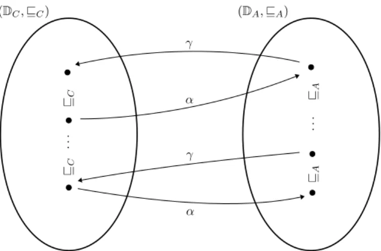
Definition 2.21 (Galois Connection) A Galois connection is a tuple (D, α, γ,

D)b

where (

D

,

v)

and (b

D

,

v)b

are partially ordered sets, α :

D7→Db

is an abstraction function and γ :

Db 7→D

is a concretization function such that α and γ are monotone and satisfy:

∀x∈D:

x

v

(γ

◦

α)(x) (2.18)

and

∀x∈Db

: (α

◦

γ)(x)

vb

x (2.19)

A Galois Insertion, in addition, satisfies:

∀x∈Db

: x = (α

◦

γ)(x) (2.20)

Monotonicity ensures that both mappings are order preserving. Property 2.18 guarantees that the abstraction is sound : The mapping into the abstract domain and back never loses information but potentially precision. Property 2.19 guarantees precision of the abstraction: The mapping into the concrete domain and back always yields a value as least as precise as the initial value. Equation 2.20 tightens these constraints:

abstraction followed by concretization maps to the original abstract value. Figure 2.2 graphically illustrates the respective mappings between the two domains

D

and

D. Theb

respective elements are ordered vertically according to the partial order relation of both posets.

To enable the applicability of the abstract domain to fixed point semantics, an abstract transformer must satisfy specific properties with regard to its concrete counterpart. Let tf : V

7→ D 7→ D

be a concrete transformer and let tf :

b

V

7→ Db 7→ Db

be an abstract transformer.

Definition 2.22 (Local Consistency) An abstract transformer tf

b

is locally consistent with a concrete transformer tf if it holds that:

∀x∈Db

:

∀u∈

V : (tf(u)

◦

γ)(x)

v

(γ

◦

tf(u))(x)

b

(2.21)

(29)

Chapter 2. Principles of Program Analysis 17 Local consistency guarantees that the abstract transfer function may be less precise than the concrete one, but it will never lose information and is therefore sound. Figure 2.3 illustrates this relation graphically. Concretization and a subsequent application of the concrete transformer is potentially more precise than the a application of the abstract transformer followed by the concretization. For a Galois insertion, γ

◦

tf

◦

α is referred to as a best abstract transformer, which may be, however, infeasible if concretization is not realizable in practice.

It remains to show that COL and MFP can equally well be applied in the abstract domain if local consistency of transformers is guaranteed. Analogously to Definition 2.8 and Definition 2.9 for concrete semantics, we define their abstract counterparts.

Definition 2.23 (Abstract Path Semantics) Let π = (u

₁

, . . . , u

_k

) be a path. Then abstract path semantics is defined as the composition of abstract transfer functions tf

b

along π such that:

J

π

K

( tf) =

b







id if π =

tf(u

b _i

)

◦J

(u

₁

, . . . , u

i−1

)

K

( tf)

b

otherwise

(2.22)

Then abstract collecting semantics for a set of paths Π and initial states S

b0 ∈ D, isb

defined as:

col(u) =

c G

s∈Sb0

G n

J

π

K

( tf)(s)

b |

π = (u

s

, . . . , u)

∈

Π

o

(2.23)

Note that in concrete collecting semantics, we assumed set union

∪

to collect all state.

For abstract states, collection of information may be performed for some other definition of union (potentially

t 6=∪).

Lemma 2.24 (Correctness of Abstract Path Semantics) Let (

D

, α, γ,

Db

) be a Galois connection, then it holds that

∀x∈D:b J

π

K

(tf)(γ (x))

⊆

γ(

J

π

K

( tf)(x))

b

(2.24) if the corresponding concrete transformer tf and abstract transformer tf

b

are locally consistent.

Proof. See [19].

Lemma 2.25 (Correctness of Abstract Collecting Semantics) Let (

D

, α, γ,

Db

) be a Galois connection, let tf

b

be an abstract transformer, S

₀∈D

and S

b₀ ∈Db

initial states such that S

0v

γ( S

b0

), then it holds that

∀u∈

V : : col(u)

v

γ ( col(u))

c

(2.25)

if for the concrete transformer tf , the abstract transformer tf

b

locally consistent.

(30)

Chapter 2. Principles of Program Analysis 18 Proof. See [19].

Reduction to abstract path-based collecting semantics (Definition 2.10) is obvious.

Also, the construction of the MFP solution (Definition 2.19) applies analogously to the abstract domain. Then Theorem 2.20 directly applies as well in the abstract domain.

To summarize, an abstraction of concrete semantics is sound if i) the abstract domain

Db

is a poset ii) abstraction α and Concretization γ are sound iii) transformers tf and tf

b

are locally consistent.

2.6 Convention and Practical Program Analysis

We will briefly address some practical aspects of program analysis. In particular, we define conventions and tools used throughout this thesis.

For convenience, we will usually define analysis problems in terms of collecting semantics. As we have seen, reduction from COL to MFP is straight forward. We denote forward semantics by col

^→

and backward semantics by col

^←

and path-based semantics by col

^→/←π

, respectively. Analogously, for the recursive equation for the MFP solution Equation 2.15, mfp

^→/←

denotes only predecessor/successor nodes in the corresponding CFG. In some cases, we restrict col and mfp to subgraphs with explicitly given source and sink nodes, or to a subset of edges. Equation 2.15 can be rewritten as:

in(u) =

G

v∈pred(u)

out(v) (2.26)

out(u) = tf(u)(in) (2.27)

which explicitly discriminates states prior and after application of a transformer, for a suitable initialization.

In practice, the least solution to the equation system above can be solved iteratively by successively updating program information in all program points by performing just one step at a time per node, cycling through all nodes (round robin).

Algorithm 2.1 Worklist algorithm for iterative data flow analysis

1 f o r u∈V do

2 in[u]←out[u]←S0

3 W ←V

4 while w6=∅ do

5 u←popW

6 in(u)←F

v∈preduout(v)

7 out(u)←tf(u)(in)

8 i f out(u) changed

9 W ←W ∪succu

Algorithm 2.1 lists a practical implementation to compute a forward MFP solution [20].

In lines 1, 2 the arrays in and out are assigned a suitable initial value, then a worklist

(31)

Chapter 2. Principles of Program Analysis 19 containing all nodes of the corresponding CFG is created (line 3). We recompute values in set in and set out, one node at a time, in some order by removing some node from W (line 5), then recompute the values (lines 6,7). If we have not reached a fixed point yet (line 8), we add the successors of the current node u (line 9) to the worklist.

If the underlying CFG is acyclic (DAG) and nodes are processed in topological order, a fixed point can be reached in time linear to the number of nodes. Consequently, if the worklist is ordered accordingly initially, a fixed point is likely to be reached quicker.

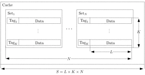
In addition, the smallest semantic unit of a program is typically a statement (or an

instruction) but not all statements affect control flow. Hence, it is customary to group

statements in basic blocks [20], which denote maximal sequences of statements with

control flow branching only at the first and the last statement, to denote a single CFG

node. More details on the general subject of practical data flow analysis can be found

in [21–23]. Note that control flow analysis [24–26] for the construction of CFG is an

important topic on its own.

(32)

Chapter 2. Principles of Program Analysis 20

(33)

Chapter 3

Context

This chapter contains background information to set this thesis into context. Every topic discussed here is related, but not necessarily a requirement to understand the remainder of this thesis. In the following the topics of real-time scheduling, aspects of hardware in real-time systems and aspects of software for real-time systems, including timing analysis of software will be addressed.

Specifically, the chapter comprises of a discussion on basics of schedulability theory in Section 3.1 and fundamentals of timing analysis in Section 3.2.

3.1 Real-time Scheduling

We start with some basic terminology. The problem of allocating processing time for concurrently running software is known as the scheduling problem. In this, the basic unit of processing is that of a task. The assignment of tasks to processors is then usually performed under a given set of constraints, which is denoted as the scheduling policy. A scheduling algorithm (or scheduler), then, is the method of finding a feasible schedule such that all tasks can be completed according to a set of constraints. A set of tasks is schedulable if for a given algorithms all constraints hold.

Real-time scheduling can typically be found in embedded systems. As opposed to non-real-time systems, the emphasis is not on load-balancing or general responsiveness but on meeting timing guarantees such as timing deadlines. Hard real-time policies give

21

(34)

Chapter 3. Context 22 firm guarantees: The consequence of deadline misses in this case is typically a complete system failure. Soft real-time policies on the other hand allow deadline misses typically at the expense of a degraded quality of service.

A schedule is preemptive if it allows the temporary suspension of a task to assign another task to the processing unit. Otherwise, a schedule is said to be non-preemptive.

If a scheduling policy allows instantaneous preemptions on demand, it is fully preemptive.

The compromise between fully and non-preemptive schedules is called deferred preemption scheduling. Under such a policy, preemption is only allowed at specific points in time or at specific program points.

Typically, tasks are being assigned priorities such that the task of highest priority is assigned to a processor. A static scheduling assigns priorities according to tasks parameters known prior to actual system execution. A scheduling is said to be dynamic if priorities are assigned at run-time. Static schedules are typically more predictable at the cost of lower performance.

Besides mere timing, additional constraints can be imposed on tasks. Precedence constraints enforce a specific order on the execution of tasks. Resource constraints impose limits on the availability of resources other than processing time, such as the mutual exclusion of accesses to certain resources.

In particular hard real-time systems pose specific requirements on the predictability of system components. Therefore, not only has the hardware and the task software to be predictable, but the scheduling algorithms themselves should be predictable in the sense that i) a safe upper bound of their processing overhead can be determined and ii) safe upper bounds on the timing behavior of the final schedule can be obtained. In the following we formally introduce the basics of uni-processor, priority-based, hard real-time scheduling without explicit precedence constraints. A general overview of hard real-time scheduling can be found in [27].

In Section 3.1.1 we define the task model used throughout the thesis, in Section 3.1.2 we address important aspects of preemptive scheduling, then we introduce two widely employed scheduling policies in Section 3.1.3. For the latter, we briefly discuss schedula- bility tests in Section 3.1.4. We further characterize issues related to task blocking and synchronization in Section 3.1.5.

3.1.1 Basic Task Model

We assume the problem of scheduling a task set

T

=

{τ₁

, τ

2

, . . .

} ⊆ N0

on a single processor. A single execution (instance) of a task is called a job where τ

_i^j

denotes the j’th job of τ

_i

.

Time in this model is discrete and measured in clock ticks if no other unit is specified

explicitly. A job can be in one of three states: ready, run and wait, as illustrated in the

automaton in Figure 3.1. The edges are labeled with the events that can occur. A job is

released once it is scheduled for execution, and placed into the ready-queue – a queue

of tasks ready for dispatch if another task is currently run by the CPU. The release of

(35)

Chapter 3. Context 23

Figure 3.1: State-machine of a task with preemption and synchronization

T

=

{τ₁

, . . . , τ

_n} ⊆N0

Task set

H

T

Hyper period

pr

_P

Priority under policy P

Task τ

i

B

_i

Blocking time

C

i

Computation time

D

i

Relative deadline

J

_i

Release jitter

R

i

Response time

T

i

Period, Inter-arrival time

U

_i

Utilization

Job τ

_i^j

a

^j_i

Arrival time

d

^j_i

Absolute deadline

f

_i^j

Finishing time

l

^j_i

Lateness

r

_i^j

Response time

s

^j_i

Starting time

Table 3.1: Task parameters

a higher priority task potentially preempts a running task. Alternatively, a job can be send into a wait state (specifically into a wait-queue ) if, for example, it fails to acquire another resource by itself. All waiting jobs receiving a signal are put back into the ready state. A task is active if there’s a job that is either ready, running or waiting. Otherwise, it is idle.

A task schedule is aperiodic if tasks are activated at arbitrary points in time. It

is periodic if activation occurs in fixed intervals or sporadic if it is aperiodic with the

constraint that there exists a minimal inter-arrival time between jobs. In the following

we only consider periodic tasks.

(36)

Chapter 3. Context 24 A task τ

i

is assigned a set of static parameters such that C

i

denotes its computation time, D

_i

its relative deadline and T

_i

its period or, alternatively, its inter-arrival time.

Release jitter is denoted by J

_i

and defines a possible imprecision in timing (e.g. time consumed by the scheduling decision and the context switch). Blocking time B

i

denotes the time span a higher priority task is prevented from execution by lower priority tasks due to deferred preemption or exclusive resource access. A deadline is an implicit deadline if D

i

= P

i

. The hyper period of a periodic task set

T

is the least common multiple of its periods T

_i

:

H

T

= lcm(T

1

, . . . , T

_k

) (3.1) The earliest release time of a job τ

_i^j

is called arrival time and is defined as:

a

^j_i

= a

^j−1_i

+ T

_i−

J

_i

(3.2)

The absolute deadline of a job is derived from the arrival time and its relative deadline:

d

^j_i

= a

^j_i

+ D

_i

(3.3)

We call the time instant at which a job executes for the first time after being released the starting time s

^j_i

and the time instant at which it completes the finishing time f

_i^j

. The response time of a job is the time span from activation to completion, defined as:

r

_i^j

= f

_i^j−

a

^j_i

(3.4)

From individual jobs, we can derive the response time R

_i

, which is defined as:

R

i

= max

j {r^j_i}

(3.5)

A task set is schedulable if all of its jobs finish before their respective deadlines:

R

i ≤

D

i−

J

i⇔

τ

i

schedulable (3.6) The time difference of finishing time and its absolute deadline is a job’s lateness:

l

_i^j

= f

_i^j−

d

^j_i

Tight integration of cache, path and task-interference modeling for the analysis of hard real time systems