Prediction of Factors Determining Changes in Stability in Protein Mutants
I n a u g u r a l - D i s s e r t a t i o n
zur
Erlangung des Doktorgrades
der Mathematisch-Naturwissenschaftlichen Fakultät
der Universität zu Köln
vorgelegt von
Parthiban Vijayarangakannan aus Dindigul (Indien)
KÖLN 2005
Berichterstatter: Prof. Dr. Dietmar Schomburg
Prof. Dr. Heinz Saedler
Tag der letzten mündlichen Prüfung: 13 Jan 2006
TABLE OF CONTENTS
1 INTRODUCTION ... 1
1.1 Preview... 1
1.2 Non-covalent Forces in Protein Stability ... 1
1.2.1 Electrostatic Interactions... 1
1.2.2 Configurational Entropy ... 5
1.2.3 Role of Water... 7
1.2.4 Hydrophobic Effect... 8
1.3 Covalent Reactions and Protein Stability... 9
1.3.1 Deamidation and Isoaspartate formation ... 11
1.3.2 Cleavage of Peptide Bonds ... 11
1.3.3 Cysteine Destruction and Thiol-Disulphide Interchange ... 13
1.3.4 Oxidation of Cysteine Residues... 13
1.3.5 Oxidation of Methionine Residues ... 14
1.3.6 Photodegradation of Proteins... 14
1.3.7 Glycation and Carbamylation of Protein Amino Groups ... 15
1.4 Protein Structural Descriptors ... 16
1.4.1 Role of Secondary Structure Elements ... 16
1.4.2 The Denatured State... 17
1.4.3 Protein/Amino Acid Packing Measures... 18
1.4.4 Protein Flexibility Measures... 19
1.5 Amino Acid Substitution Matrices... 20
1.5.1 Empirical substitution models ... 21
1.5.2 PAM matrices ... 21
1.5.3 Dayhoff matrices... 22
1.5.4 JTT matrices ... 22
1.5.5 Other empirical models... 22
1.5.6 Blosum (Block substitution matrices) ... 22
1.5.7 Poisson models ... 23
1.6 Energy Functions... 23
1.6.1 Experimental Protein Denaturation ... 23
1.6.2 Oxidants and Reductants ... 26
1.6.3 Free Energy Derivation... 26
1.6.4 ∆∆G and ∆∆GH2O ... 27
1.6.5 Theoretical Background... 29
1.7 Experimental Substitution Methods... 30
1.7.1 Site-Specific Mutagenesis... 30
1.7.2 Random Mutations at Specified Positions... 30
1.7.3 DNA Shuffling... 30
1.7.4 Protein Stability Assessment ... 31
1.8 Uses of Predicting Protein Stability ... 32
1.8.1 Increased Thermostability... 32
1.8.2 Decreased Stability / Thermosensitivity... 32
1.8.3 Mutations and Drug Targets ... 32
2 LITERATURE REVIEW ... 34
2.1 Use of Empirical and Statistical Energy Functions ... 35
2.1.1 Protein Structure Solutions ... 35
2.1.2 Protein Folding ... 36
2.2 Stability Assessment ... 37
2.2.1 Protein Structure Quality ... 38
2.3 Theoretical Prediction Models ... 38
2.3.1 Empirical Energy Functions and Prediction Models... 39
2.3.2 Statistical Energy Functions ... 41
2.3.3 Neural Networks ... 43
2.3.4 Support Vector Machines ... 43
2.4 Application Note ... 44
2.4.1 PopMuSIC ... 44
2.4.2 Fold-X... 44
2.4.3 I-Mutant (version 1 and 2) ... 44
2.4.4 DMutant ... 45
3 MATERIALS AND METHODS... 46
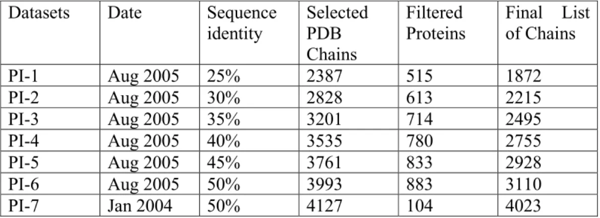
3.1 Structural Training Datasets... 46
3.1.1 Selection... 47
3.1.2 Filters ... 48
3.2 Mutation Datasets... 49
3.3 Statistical Potentials ... 50
3.4 Distance Dependent Pair Potential... 50
3.4.1 Radial Distribution of atoms... 50
3.4.2 Distance Cutoff ... 51
3.4.3 Atom Classification Models (Atom Types)... 51
3.5 Torsion Angle Potential ... 57
3.5.1 Basic Construction... 57
3.5.2 Optimisation... 58
3.6 Protein Environment Specificity ... 59
3.6.1 Amino Acid Compactness ... 59
3.6.2 Secondary Structure Specificity... 60
3.7 Statistical Methods ... 62
3.7.1 Simple Linear Regression... 62
3.7.2 Multiple Linear Regression ... 63
3.7.3 Multicolinearity Diagnostics... 64
3.7.4 Stepwise Linear Regression... 65
3.7.5 Final Prediction Model ... 65
3.7.6 Assessment of Overall Prediction Efficiency ... 66
3.7.7 Validation of Prediction Model ... 67
4 RESULTS AND DISCUSSION ... 69
4.1 Construction of Statistical Potentials ... 69
4.1.1 Structural Training Datasets ... 69
4.1.2 Distance Dependent Pair Potential ... 70
4.2 The Prediction Model... 82
4.2.1 Mutation Datasets ... 82
4.2.2 Simple Linear Regression... 82
4.2.3 Multiple Linear Regression ... 82
4.2.4 Classifying the Protein Environment... 86
4.2.5 Multicollinearity Diagnostics ... 89
4.2.6 Stepwise Linear Regression... 90
4.3 Prediction Model Analyses ... 97
4.3.1 Comparison of Structural Training Datasets ... 97
4.3.2 Comparison of Atom Classification Models ... 99
4.3.3 Effect of Torsion Angle Potentials ... 104
4.3.4 Gaussian Apodisation ... 105
4.3.5 Evaluating Structural Training Datasets for Torsion Potentials106 4.3.6 Distinguishing the Structural Regions ... 109
4.3.7 Short, Medium and Long Distance Ranges ... 112
4.4 Prediction Model Validation ... 114
4.4.1 Split-sample validation ... 115
4.4.2 k-fold cross-validation ... 115
4.4.3 Jack-knife Test and Outliers ... 118
4.5 Comparison with Other Models ... 120
4.6 Public World Wide Web Access... 122
APPENDICES ... 123
Appendix A: Abbreviations ... 123
Appendix B: Symbols/Units ... 124
Appendix C: Amino Acid Properties... 125
TABLE INDEX ... 126
FIGURE INDEX... 128
PUBLICATIONS... 131
ACKNOWLEDGEMENT ... 132
REFERENCES... 133
ZUSAMMENFASSUNG... 140
SUMMARY ... 142
ERKLÄRUNG ... 144
LEBENSLAUF ... 145
1 INTRODUCTION
1.1 Preview
The relationship between the conformational stability and chemical integrity of a protein is of particular importance to understanding the mechanisms of protein folding and inactivation. On exposure to changes in environmental conditions (elevated temperatures, acidic/basic conditions, or the presence of structure perturbing solutes), protein molecules may undergo either conformational changes (local changes in secondary and tertiary structure), reversible unfolding (cooperative loss of higher ordered structure), or inactivation (irreversible changes in structural or chemical integrity of the molecule). Perturbation of protein structure often leads to the exposure of previously buried amino acid residues, facilitating their chemical reactivity. In many cases, partial unfolding of a protein is often observed prior to the onset of irreversible chemical or conformational processes. Moreover, protein conformation generally may control the rate and extent of deleterious chemical reactions. Conversely, chemical changes to the polypeptide backbone or amino acid side chains of a protein may lead to loss of conformational stability. For instance, the reduction of disulphides or the oxidation of cysteine residues can induce protein unfolding and aggregation. The interplay between these reactions and protein conformation is crucial to emphasise the understanding of protein stability.
1.2 Non-covalent Forces in Protein Stability
1.2.1 Electrostatic Interactions
(i) Van der Waals Interactions and Electronic Shell Repulsion
Van der Waals interactions, also known as London dispersion forces, result from attractive transient oscillating diploes that non-bonded atoms induce in each other. This transient dipole is generated by electrons moving in relation to the nucleus. In a pair of atoms each dipole polarizes the opposing atom. The attraction energy is proportional to r-6, the distance between the nuclei, and to
the polarisability of the atoms. Such interactions, also ubiquitous, are fairly weak and short range. Because of the strong distance dependence of van der Waals interactions, the packing of atoms in the protein core, relative to their interaction with solvent, is important in determining whether they will stabilise or destabilise the native state.
The electronic shell repulsion is due to sterical hindrance when neighbouring atoms start to have overlap of the electron clouds. The repulsion of the electronic shells is proportional to r-12. The attractive (distant) and the repulsive (close) components are usually taken together and described by the Lennard- Jones potential. Electrostatic repulsion may be more important, not only in destabilising the native state but also in terms of its effect on the degree of extension of the unfolded state.
A series of simplifications have been made in calculating van der Waals interactions. Mainly, only atoms in contact are taken as the close neighbours that must be considered. Also, electrostatic interactions are simplified with regard to geometry of interactions. These simplifications result in a van der Waals potential which is isotropic (equal in all directions) and is a function solely of contact distance. The values of the partial charges are subject to large inaccuracies. The complete expression for dispersion forces and electron repulsion is given below:
Evdw,ij = -A/rij6 + B/rij12 (1)
Here A and B are constants depending on the atoms. The parameter, B, is taken from the sum of van der Waals radii; the parameter, A, is from the polarisability of the atoms. The resulting minimum corresponds to the most favourable atomic distance.
(ii) Hydrogen Bonding
Whenever two heavy (non-hydrogen) atoms with opposite partial charges [donor (D)-acceptor(A) pairs] were found to be within a distance (d) of 3.5Å, a hydrogen bond has been inferred. The geometrical goodness of the hydrogen
(1) Angle θD between vectors BD-D and D-A, BD is the atom covalently bonded to the donor (D) atom.
(2) Angle θA between vectors D-A and A-BA, BA is the atom covalently bonded to the acceptor (A) atom.
A hydrogen bond was taken to have good geometry if both of these angles lie in the range of 90-150°. The distance d also slightly varies according D-A pairs. Hydrogen bonding is quite sensitive to distance constraints. Hydrogen bonds between NH-O, OH-N and OH-O need an approximate distance range of 2.55-3.04Å, 2.62-2.93Å and 2.65-2.93Å respectively. The amount of energy one hydrogen bond contributes towards the stabilisation of a protein is calculated to be around 1-3 kcalmol-1.
(iii) Salt Bridges (Ion Pairs)
Salt bridges or ion-pairs are a special form of particularly strong hydrogen bonds made up of the interaction between two charged residues. On the other hand, there are also non-hydrogen bonded salt bridges and this discrimination is solely based on geometric considerations. In folded proteins, pairs of neighbouring, oppositely charged residues often interact to form salt bridges.
Salt bridges play important roles in protein structure and function such as in oligomerisation, molecular recognition, allosteric regulation, domain motions, and α-helix capping (Kumar and Nussinov 1999). An early calculation (Honig and Hubbell 1984) estimated that the cost of transferring a salt bridge from water to the protein environment is approximately 10-16 kcal/mol. Using continuum electrostatic calculations, it has been shown that the desolvation penalty due to the burial of polar and charged groups in the protein interior (a low dielectric environment) during protein folding, may not be fully recovered by favourable electrostatic interactions in the folded (Hendsch and Tidor 1994) state. Salt bridges can be stabilising or destabilising to the protein structure depending on their geometry, location in the protein, electrostatic interaction between salt-bridging side-chains with each other, and that between the salt bridge and its surroundings. But, most of the salt bridges are stabilising
irrespective of whether they are buried or exposed, isolated or networked, hydrogen bonded or not.
Salt bridge formation is inferred for a pair of oppositely charged residues (Asp or Glu with Arg, Lys or His) if they meet the following criteria (Kumar and Nussinov 1999):
(1) The centroids of the side-chain charged groups in oppositely charged residues lie within 4.0Å of each other.
(2) At least one pair of Asp or Glu side-chain carboxyl oxygen atoms and side-chain nitrogen atoms of Arg, Lys or His are within a 4.0Å distance.
The location of residues forming salt bridges is characterised in terms of the solvent accessible surface areas (ASA) (Lee and Richards 1971; Tsai and Nussinov 1997) of their constituent residues, with a probe radius of 1.4Å. The location of a salt bridge in the protein is estimated by the average ASA of the salt bridge. The average ASA of a salt bridge is average of the ASAs of the two salt-bridging residues. A salt bridge is classified as being buried in the protein core if it has an average ASA of ≤20%, otherwise it is classified as being exposed to the solvent. A salt bridge between two charged residues is considered to be networked if at least one of these charged residues forms additional salt bridge(s) with other charged residue(s) in the protein. Otherwise, the salt bridge is considered to be isolated.
The geometry of a salt bridge is characterised in terms of the distance between the centroids of the salt-bridging residue side-chain charged groups, and the angular orientation of these groups with respect to each other. The angular orientation of the side-chain charged groups in the two salt-bridging residues is computed as the angle between two unit vectors. Each unit vector joins a Cα atom and a side-chain charged group centroid in a salt bridging residue.
(iv) Other Electrostatic Interactions
Electrostatic interactions occur between charges on protein groups. Such charges are present at the amino- and carboxy- termini and on many ionisable
side chains. Charges buried in the protein interior will interact strongly since the protein interior is considered a low-dielectric medium. Van der Waals interactions are also electrostatic that involve transient dipoles. This may also occur due to the presence of permanent dipoles and have similar effects.
π-π (aromatic-aromatic) interactions between the aromatic groups are important in protein structures. Phe-Phe interactions is a good example of these interactions. However, they occur almost exclusively in electrostatically attractive geometries. Electrostatically unfavourable regions are only sparsely populated. Electrostatics dominate the geometry of interaction, while van der Waals' interactions are less significant due to the hydrophobic environment of the protein core.
Cation-π interactions are also important for protein folding. A cation-π interaction is a noncovalent binding force of broad importance in biological systems and in supramolecular chemistry. It is defined as the attraction between a cation and the face of a simple π system, such as in benzene or ethylene. The physical origin of the cation-π interaction is primarily electrostatic, involving an attraction of the cation to a locus of negative electrostatic potential associated with the face of the π system. It is a common and pervasive contributor to protein secondary structure and to a wide range of small molecule and macromolecule binding interactions in biology. Within a protein, cation-π interactions (Gallivan and Dougherty 1999) can occur between the cationic sidechains of either lysine (Lys, K) or arginine (Arg, R) and the aromatic sidechains of phenylalanine (Phe, F), tyrosine (Tyr, Y) or tryptophan (Trp, W). But, histidine can participate in cation-π interactions as either a cation or as a π-system, depending on its protonation state.
1.2.2 Configurational Entropy
Whereas the interactions discussed above tend to stabilise the native protein structure, configurational entropy destabilises it. The gain in configurational entropy relates to the increased degrees of freedom available to the protein chain in the unfolded state relative to the native state. This gain comes from
both the side chains and the backbone. Although the peptide backbone of most residues in a globular protein is relatively fixed (i.e., has low entropy), those residues that are most buried within the core of the protein have even fewer backbone degrees of freedom. The entropic effect of burying side chains is more pronounced since they have considerable flexibility on the protein surface. As larger proteins bury more of their side chains, they will have an overall larger configurational entropy change per residue. This effect may help to set a limit on the size of a globular folding domain.
The amino acid configuration also affects the configurational entropy. For instance, proteins containing large proline residues will have lower entropy in the unfolded state and thus will be more stable. The opposite will be true for proteins containing a large proportion of glycine.
(1) Entropy Cost of Fixing a Backbone
The backbone entropy term is normally used to account for the entropy cost of fixing a residue backbone. This can be different for the residues that are present in organised secondary structure regions and in loops without secondary structure due to increased flexibility of residues in loops. Compactness measures of residues are normally used to distinguish the residues in loops (Guerois et al. 2002) to assess the backbone entropy. ASA (Accessible Surface Area) and atom packing information are widely used to classify the residues in these cases (Gromiha et al. 1999b). Hydrogen bonding efficiency of specific residues is also used. If both the nearby residues can form backbone-backbone H-bond between each other, they are considered to have lower configurational entropy. Comparatively higher configurational entropy is assumed for two nearby residues that are not involved in backbone-backbone H-bonds (Guerois et al. 2002).
(2) Entropy Cost of Fixing a Side chain
Side chain entropy depends on the mobility of the side chains, which in turn directly depends on the solvent accessibility of the residues in side chains.
Decreased solvent accessibility reduces the mobility and packs the side chain.
This entropy term also depends on the ability of side chain residues to form hydrogen bonds or exhibit strong electrostatic forces with the adjacent residues (Bromberg and Dill 1994). If the entropy cost is bigger than the favourable interaction energy brought by the hydrogen bond and the electrostatic interactions, neither these interactions nor the entropy of the side-chain can be assessed efficiently (Guerois et al. 2002).
1.2.3 Role of Water
Water plays a crucial role in the stabilisation of proteins. The small molecular size of water relative to other liquids, along with its complex hydrogen bonded structure, makes it a good solvent for many functional groups (Shirley 1995).
These same features also give rise to hydrophobic effect which has got more than one definition in literature (Shirley 1995):
(1) Transfer of a compound from an organic liquid to water.
(2) Transfer of apolar surface from any initial phase into water.
(3) Transfer into water accomplished by a large ∆Cp.
Considering protein stability, the hydrophobic effect refers to energetic consequences of removing apolar groups from the protein interior and exposing them to water. So, the second definition is considered to be more relevant. The term hydration is considered to be the transfer of any group from gas phase to water. Though, hydration and hydrophobic effect are described separately, some of the other interactions are described here:
(1) Atomic Solvation Parameters
Atomic solvation parameters (ASPs) can be explained as transfer energies from water to the protein interior (Lomize et al. 2002). They can be effectively used to incorporate the role of water in protein structure and stability assessment.
Studies are available which suggest that the protein core can be approximated using atomic solvation parameters. The polarity of different atom types, that is, the rank order of their transfer energies from water to the different media, was identical for protein and organic solvents (Cali < Caro < S < N < O). However,
the absolute values and even the signs of ASP were strongly environment dependent. If mean force potentials (MFPs) are protein environment dependent based on solvent parameters (e.g., solvent accessibility), it will be more accurate than the environment independent potentials.
(2) Water molecules forming Hydrogen Bonds
Water molecules form hydrogen bonds, both in the folded and unfolded state with the primary and secondary structures of proteins. The calculation of the effect of hydrogen bonding water in protein stability is a complex issue.
Several experimental studies show that the deletion of polar atoms that make hydrogen bonds with a partially or fully buried water molecule can have a large destabilising effect on the protein interaction. (Takano et al. 1997;
Grantcharova et al. 2000; Covalt et al. 2001). It may be sensible to define a water bridge as a water molecule that makes more than two hydrogen bonds with the protein. Removing one of the polar groups involved in a water bridge may exclude the bound water from a particular site of the protein and induce the desolvation of the other polar groups partners of the water molecule. Thus, it is important to determine the water positions and its ability to form hydrogen bonds with protein structures.
1.2.4 Hydrophobic Effect
During protein folding, the transition from the unfolded state (with several short-lived intermediates) to a single native state is accompanied by the burial of solvated nonpolar side chains (and polar peptide units) into the nonsolvated core of the protein. The "hydrophobic effect" or "hydrophobic interaction" in protein structure is derived from the combined properties of H-bonds in water and van der Waals forces applied to amino acid residues with nonpolar side chains. A nonpolar side chain in water makes less favourable van der Waals interactions than if it was dissolved in an apolar solvent. In addition, the solvating water molecules cannot satisfy their four potential H-bonds while they surround an apolar solute. In contrast, a nonpolar side chain in an apolar core of a protein has gained favourable van der Waals interactions and has rid
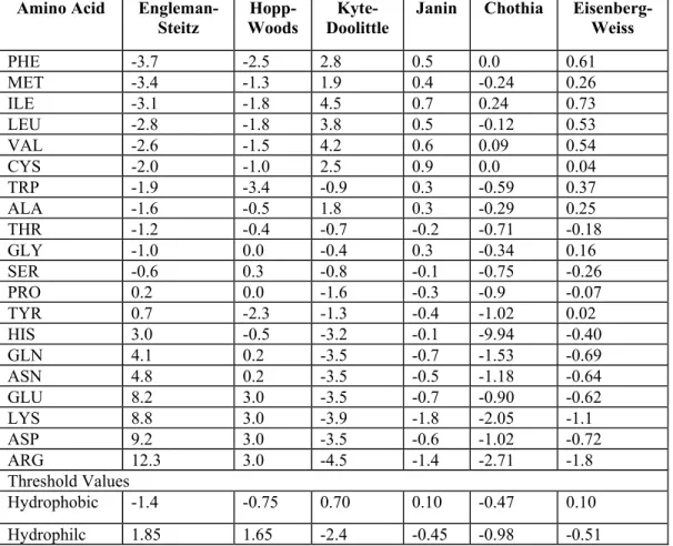
itself of the dissatisfied solvating water. The interior of folded proteins is tightly packed. Residue specific hydrophobicity scales were derived by several people to quantify the hydrophobic effect of proteins. Sequence specific plots were also generated using these hydrophobicity scales (Table 1). The solvent accessibility of the amino acids was used in this study to classify the amino acids from structural training datasets and mutations. These hydrophobicity values are highly correlated with ASA of the amino acids. So, these values can also be used for classifying amino acids instead (Muyoung et al. 2005).
Amino Acid Engleman- Steitz
Hopp- Woods
Kyte- Doolittle
Janin Chothia Eisenberg- Weiss PHE -3.7 -2.5 2.8 0.5 0.0 0.61 MET -3.4 -1.3 1.9 0.4 -0.24 0.26 ILE -3.1 -1.8 4.5 0.7 0.24 0.73 LEU -2.8 -1.8 3.8 0.5 -0.12 0.53 VAL -2.6 -1.5 4.2 0.6 0.09 0.54 CYS -2.0 -1.0 2.5 0.9 0.0 0.04 TRP -1.9 -3.4 -0.9 0.3 -0.59 0.37 ALA -1.6 -0.5 1.8 0.3 -0.29 0.25 THR -1.2 -0.4 -0.7 -0.2 -0.71 -0.18 GLY -1.0 0.0 -0.4 0.3 -0.34 0.16 SER -0.6 0.3 -0.8 -0.1 -0.75 -0.26 PRO 0.2 0.0 -1.6 -0.3 -0.9 -0.07 TYR 0.7 -2.3 -1.3 -0.4 -1.02 0.02 HIS 3.0 -0.5 -3.2 -0.1 -9.94 -0.40 GLN 4.1 0.2 -3.5 -0.7 -1.53 -0.69 ASN 4.8 0.2 -3.5 -0.5 -1.18 -0.64 GLU 8.2 3.0 -3.5 -0.7 -0.90 -0.62 LYS 8.8 3.0 -3.9 -1.8 -2.05 -1.1 ASP 9.2 3.0 -3.5 -0.6 -1.02 -0.72 ARG 12.3 3.0 -4.5 -1.4 -2.71 -1.8 Threshold Values
Hydrophobic -1.4 -0.75 0.70 0.10 -0.47 0.10 Hydrophilc 1.85 1.65 -2.4 -0.45 -0.98 -0.51
Table 1: Hydrophobicity (amino acid specific) scale values derived from various studies (Chothia 1974; Janin 1979; Hopp and Woods 1981; Kyte and Doolittle 1982; Eisenberg et al. 1984; Engelman et al. 1986).
1.3 Covalent Reactions and Protein Stability
The covalent modification of proteins in vivo has been proposed as a natural mechanism to designate enzymes for turnover. Both enzymatic and nonenzymatic pathways of posttranslational modification of proteins have been identified. Spontaneous, nonenzymatic reactions include the deamidation of
asparangynyl residues, racemisation of aspartyl residues, isomerisation of prolyl residues, and glycation of amino acids, as well as site specific metal catalysed oxidations. Enzymes have been identified in vivo that specifically interact with covalently modified proteins, including caboxymethyl transferase and alkaline protease. It has been proposed that covalent changes caused by in vivo protein oxidation are primarily responsible for the accumulation of catalytically compromised and structurally altered enzymes during aging. In addition, protein oxidation may play a role in several pathological states, including inflammatory disease, atherosclerosis, neurological disorders, and cataractogenesis.
The relationship between the conformational stability and covalent reactions of a protein is of particular importance to the understanding of the mechanisms of protein activation/inactivation. On exposure to changes in environmental conditions (elevated temperature, acidic/basic conditions, or the presence of structure perturbing solutes), protein molecules may undergo conformational changes (local changes in secondary and tertiary structure), or inactivation (irreversible changes in structural or chemical integrity of the molecule).
Perturbation of protein structure often leads to the exposure of previously buried amino acid residues, facilitating their chemical reactivity. In fact, partial unfolding of a protein is often observed prior to the onset of irreversible chemical or conformational processes (Shirley 1995). Moreover, protein conformation generally may control the rate and extent of deleterious chemical reactions. Conversely, chemical change to the polypeptide backbone or amino acid side chains of a protein may lead to loss of conformational stability. For example, the reduction of disulphides or the oxidation of cysteine residues can induce protein unfolding and aggregation which plays a considerable role in the denaturation of proteins. Obviously, this coupled interaction between these two phenomena has the potential to complicate studies of protein folding and unfolding significantly.
During the protein engineering and other solutions related to the analysis of protein folding and stability, these reactions should invariably be considered
with importance to identify chemical degradation in proteins and minimise its occurrence.
1.3.1 Deamidation and Isoaspartate formation
The spontaneous, nonenzymatic deamidation of asparagines residues is one of the most commonly encountered chemical modifications of proteins.
Deamidation can occur in acidic, neutral, or alkaline conditions, although the chemical mechanism of hydrolysis is strongly dependent on pH. The biological purpose of deamidation in vivo may involve the regulation of protein degradation and clearance, thus serving as a type of biological clock. Naturally occurring protein methyl transferases have also been identified that specifically modify deamidated by-products, perhaps by tagging damaged protein for either repair or clearance.
By examining the amide loss for a large series of synthetic pentapeptides of sequence (Gly-X-Asn-X-Gly and Gly-X-Gln-X-Gly) under physiological conditions, the enhanced lability of peptide amides compared to simple aliphatic amides was demonstrated (Robinson and Rudd 1974). The asparagines containing peptides were observed to deamidate faster than glutamine counterparts. Direct hydrolysis of amide linkages was found to be slow due to the presence of an intramolecular mechanism in which, under neutral to basic conditions , the peptide bond nitrogen attacks asparanginyl carbonyl residues, causing ring closure with concomitant release of ammonia.
The resulting five-membered succinimide is unstable and susceptible to subsequent hydrolysis which, in turn leads to the formation of α- and β-aspartyl residues. Under acidic conditions, deamidation thought to proceed by direct hydrolysis, resulting in the formation of α-aspartyl residues alone. Asn-Gly and Asn-Ser sequences were found to be particularly labile owing to decreased steric hindrance of succinimide formation by C-terminal residues.
1.3.2 Cleavage of Peptide Bonds
The cleavage of a peptide disrupts the linear sequence of amino acid residues within a protein chain. This covalent modification, however, may or may not
affect higher ordered structure of a protein and its biological activity. There are numerous examples of both non-specific hydrolysis and proteolysis leading to extensive protein degradation as well as specific proteolytic clips activating precursor forms of enzymes. Conversely, since the intramolecular interactions responsible for tertiary structure formation are sufficiently strong (cooperative), the introduction of a single intrachain clip in the polypeptide backbone may have little or no effect on a protein’s structure or function.
Three major mechanisms of peptide bond cleavage have been identified (Shirley 1995):
(1) Preferential hydrolysis of peptide bonds at aspartic acid residues under acidic conditions.
(2) At more physiological pH, C-terminal succinimide formation at Asn residues.
(3) Enzymatic proteolysis including autolysis.
The preferential hydrolysis of a peptide bond at Asp residues is generally believed to occur at the C-terminal side of this residue in polypeptide chains.
The carboxyl group side chain of Asp catalyses the cleavage reaction by acting as a proton donor at pH values below the pKa of the carboxyl group. The Asp- Pro bond is known to be particularly labile due to more basic nature of the proline nitrogen. Cleavage of polypeptide can also occur under physiological conditions. Analogous to the deamidation reaction discussed previously, succinimide formation at asparagine residues can potentially lead to the spontaneous cleavage of polypeptide chains. In this case, the side chain amide nitrogen attacks the peptide bond to form a C-terminal succinimide residue and a newly formed amino terminus. This type of cleavage has been reported to occur in both model peptides and in proteins (Tyler-Cross and Schirch 1991).
Contaminating proteases are often found to cleave recombinant proteins during both fermentation and purification. Strategies to limit proteolysis include the addition of protease inhibitors, careful selection of cell host including protease negative mutants, sequence modification of susceptible sites in target proteins,
and optimisation of fermentation and purification conditions. Storage of purified proteases under certain conditions may also lead to peptide bond cleavage (autolysis).
1.3.3 Cysteine Destruction and Thiol-Disulphide Interchange
Cysteine residues are naturally occurring crosslinks that covalently connect polypeptide chains either intra- or intermolecularly. Disulphides are formed by the oxidation of thiol groups of cysteine residues by either thiol disulphide interchange or direct oxidation. The probability of formation of a disulphide bond will depend on both the intrinsic stability of potential cysteine residues to free cysteines and the conformation of the protein molecule. Intracellular proteins usually lack such crosslinks and their atypical presence commonly reflects a role in an enzyme catalytic mechanism or involvement in the regulation of its activity. In contrast, extracellular proteins frequently contain disulphide bonds, probably reflecting the need for the increased stability of such proteins. The destruction of cysteine residues in proteins have been shown to proceed by a base catalysed (β-catalysed) reaction in alkaline media (pH 12- 13). Protons on polypeptide α-carbon atoms are relatively labile at high pH, since it is attached to two electron withdrawing groups (-CONH-, -NHCO-).
This β-elimination results in the formation of two unstable intermediates, dehydroalanine and thiocysteine (Whitaker and Feeney 1983). The same reaction can occur at neutral pH and elevated temperatures and has been shown to contribute irreversible thermoinactivation of ribonuclease and lysozyme at pH 6-8 and 90-100° C (Ahern and Klibanov 1988).
1.3.4 Oxidation of Cysteine Residues
The relative stability of a reduced cysteine residue and its oxidised disulphide counterpart depends on the redox potential of a protein’s environment. In vivo, the electron donors and acceptors that interact with protein thiols and disulphides are primarily other thiols and disulphides (e.g., as reduced and oxidised glutathione). These compounds catalyse disulphide exchange reactions, resulting in the most thermodynamically favourable redox status of
protein’s cysteine residues (free thiols vs disulphides). Redox buffer containing oxidised and reduced thiol compounds are used to catalyse the cysteine residues with the resultant reshuffling of disulphide bonds leading to the formation of the native protein. Reducing agents (eg. dithiothreitol) are also sometimes used to maintain cysteine residues in their active, reduced form.
Some metal ions (e.g., copper, iron) at elevated pH also catalyse oxidation to form inter and intra-molecular disulphide bonds together with some non- molecular byproducts such as sulphenic acid. Purification and storage of proteins containing naturally reduced cysteine often produces inactivation (eg.
acidic fibroblast growth factor).
1.3.5 Oxidation of Methionine Residues
The oxidation of methionine residues has been associated with the loss of biological activity in a number of peptides and proteins (Swaim and Pizzo 1988). During oxidation, this thioether is converted to its sulphoxide counterpart. This is a reversible reaction in which methionine residue can be regenerated either by reducing agents or enzymatically. Harsher oxidative conditions cause irreversible formation of methionine sulphone. In vitro, proteins are commonly treated with dilute hydrogen peroxide (H2O2) solution or stronger oxidisers to achieve methionine oxidation. In vivo, oxygen containing radicals, such as superoxide, hydroxyl, and H2O2, are generated in a variety of cells (e.g., neutrophils), leading to the oxidation of several amino acids, including methionine, with potential implications for various aging or disease related processes (Swaim and Pizzo 1988).
1.3.6 Photodegradation of Proteins
Both ionising and non-ionising radiation can cause protein inactivation. The effects of different types of ionising radiations (γ-rays, X-rays, electrons, α- particles) on a protein molecule (in both solid and solution states) have been examined in detail because of interest in the use of radiation as a potential sterilisation technique in the food industry (Shirley 1995). Both direct effects and indirect effects (radiolysis of water or buffer salts and subsequent protein
alterations) have been extensively documented and recently reviewed.
Nonionising radiation, such as UV light, may also cause irreversible damage to protein molecules. These effects are of particular concern biologically in understanding the mechanism of cataract formation and sunburn damage. In addition, protein unfolding/refolding studies frequently utilise UV/visible and fluorescence spectroscopy as methods of detection in which the potential adverse effects of incident light on proteins must be controlled and minimised.
The amino acids tryptophan, tyrosine and cysteine are particularly susceptible to UV-A and UV-B photolysis. The absorption of photons leads to photoionisation and the formation of photodegradation products either by direct interaction with an amino acid or indirectly via various sensitising agents. (such as dyes, riboflavin, or oxygen).
1.3.7 Glycation and Carbamylation of Protein Amino Groups
Sugars are frequently used as stabilisers of proteins during storage in solution or as lyophilised powders. Reducing sugars can covalently react with protein amino groups (e.g., the ε-amino groups of lysine residues or the amino group of N-terminus of polypeptide chains), which may lead to irreversible changes in conformation and stability of proteins. When a reducing sugar, such as glucose is incubated over long periods, the spontaneous formation of a Schiff’s base between protein amino groups and glucose is often observed. Through a series of subsequent reactions known as the Amodori rearrangement, covalent adducts are then formed. This process is frequently referred to as Maillard reaction or nonenzymatic browning. These Maillard adducts can further degrade to form so-called “advanced glycosylation end products” (AGEs), resulting in both protein crosslinking and the appearance of fluorescent byproducts. These glycation reactions are believed to be involved in degenerative processes in vivo.
Protein amino groups are also reactive with isocyanate ions leading to carbamylation of proteins (Stark 1965). Urea is in equilibrium with isocyanate ions. Therefore, protein unfolding experiments using this denaturant should be
done with freshly prepared urea and with minimised period of contact between urea and protein.
1.4 Protein Structural Descriptors
1.4.1 Role of Secondary Structure Elements
The main SSEs (Secondary Structure Elements), helices and strands, are formed by hydrogen bonds. Thus, a hydrogen bonding potential becomes very useful in empirical potentials. Helices are formed by hydrogen bonds between residues in the same helix. Three different helices exist, but only α-helix is more common than the others. The bonds forming helices restrict the torsion angles, and the idealised angles for ‘geometrically correct’ α-helix are φ = - 57.8 and ψ = -47.0. However, the real angles usually deviate from these.
Strands and sheets are formed by successive hydrogen bonds between residues which can be far apart in sequence (Table 2). The backbone hydrogen bonding groups (N-H and O=C) are in the plane of the sheet, with the bonding groups from successive residues pointing in opposite directions. Let residue i be in one strand, and residue j in another. Then, the bonding of two strands can be either parallel or antiparallel. Parallel bonding is formed by each residue forming hydrogen bonds to two residues on the other strand, separated by a residue in the sequence (successive H-bonds). Antiparallel bonding is formed by each residue forming two hydrogen bonds with a single residue on the other strand (successive hydrogen bonds). Sheets can be parallel, antiparallel or mixed (with both parallel and antiparallel bondings). The idealised strand satisfying these constraints can be thought of as a helix with two residues per turn, with torsion angle of approximately φ = -120 and ψ = +120.
Distance matrices can be useful, either manually or automatically, to indicate where there can be SSEs. For idealised α-helices, the distance between the Cα atoms from the start of the helix can be roughly calculated to be 3.8, 5.4, 5.1, 6.3, 8.7, 9.9, 10.6, 12.5, ….. These distances are found by idealised angle pair for α-helices and the distances between the backbone atoms. Real helices
usually deviates from these due to irregularities. In a distance matrix, a helix will turn up as an area of small distances along the main diagonal.
For an idealised β-strand the successive distances from a residue i can be calculated to be 3.8, 6.6, 10.3, 13.5, 16.9, …… Real strands also deviate from these values.
Thus, the development of compactness (of amino acids) and SSE (secondary structure element) specific statistical potentials from radial pair distribution of atoms and torsion angles must be more accurate and their coarse grained nature produces a high definition of protein structure and stability.
SSEs H-bond order
α-Helix H-bond(i, i+4), H-bond(i+1, i+5), ……
310-Helix H-bond(i, i+3), H-bond(i+1, i+4), ……
Helices
π-helix H-bond(i, i+5), H-bond(i+1, i+6), ……
Parallel H-bond(i, j), H-bond(j, i+2), H-bond(i+2, j+2), H-bond(j+2, i+4), ……
Sheets
Antiparallel H-bond(j, i), H-bond(i, j), H-bond(j+2, i+2), H-bond(i+2, j+2), ……
Table 2: Conservation of H-bond order in SSEs (secondary structure elements).
1.4.2 The Denatured State
For most proteins, the denatured state is insoluble and many of the physical techniques available for characterising it (in solution) are relatively insensitive for detecting its structure that has a highly flexible, dynamic character. In the absence of any evidence, it was only simple to assume that it is a featureless random coil state. It was also essential to interpret the experimental data because the energetics of protein’s native state achieves a larger role only when it’s assumed to be a random coil. In effect, the experimentally measured thermodynamic parameters reflect the entire process of protein folding, with the sum (Shortle 1996) of protein interactions in the native state supplying all the free energy needed to derive the formation of structure. In spite of some attempts to explain the role of the denatured state, more concrete evidences are needed to understand the definitive nature of its involvement in protein folding and stability.
The denaturing agents play a dominant role with denatured state rather than the native state. Some of the denaturing agents like SDS have a close interaction with denatured state. These amphipathic compounds interact almost exclusively with the denatured state (3), because most of the hydrophobic surface to which they bind becomes available only when the native state breaks down. Although the details of the chemistry underlying the action of solvent denaturants like urea and guanidine hydrochloride are still poorly understood at phenomenological level, their mechanism of action is thought to involve weak binding or adsorption to nonpolar surfaces (4, 5). Because much more nonpolar surface is exposed in the denatured state, urea and guanidinium ion promote the dissociation and unfolding of proteins through their more extensive association with the denatured state.
1.4.3 Protein/Amino Acid Packing Measures
The compactness of a protein can be defined as the ratio of solvent accessible area of the protein and the surface area of a sphere with equal volume to the protein. Assuming that most proteins are more or less globular in shape, a better packed protein will have a smaller ratio value. For analysing point mutations associated with single amino acids, it becomes important to analyse the compactness of a single amino acid. Some of the packing measures are given below:
(1) It can be described as the relative ASA which is derived as the ratio between the real ASA of an amino acid in native state and the constant ASA of the same amino acid in ALA-X-ALA extended state.
(2) Other measures of compactness are also available which prove to be viable in certain cases of protein structure prediction methods. It is derived as the distribution of Cβ or Cα atoms around any amino acid. The number of Cβ atoms in a distance of 6-8Å can be calculated, where the compactness is directly proportional to the number of selected atoms at a defined cutoff distance.
1.4.4 Protein Flexibility Measures
Dynamics of proteins plays an important role in function of proteins (Brooks et al. 1988). Stability of a protein after a point mutation, flexibility of protein environment may have a considerable role to accommodate the mutated amino acid in any specific position. However, assessing protein flexibility of the mutated region is necessary to include its effect.
One of the earliest attempts to accommodate small changes in conformation were through the use of implicit methods (Jiang and Kim 1991) for protein- ligand docking studies. The protein is held fixed, but a “soft”-scoring function is used to evaluate the fit of the ligand to the receptor. Often, scoring functions are derivatives of force fields from molecular mechanics, modified for use in a new application. Soft functions allow for some overlap between the ligand and the protein, giving a small estimate of the plasticity of the receptor. Protein structural stability or rigidity is also highly correlated with protein unfolding (Rader et al. 2002).
The ideal method to predict protein flexibility is to perform molecular dynamics simulation of proteins in aqueous solution with an accurate physical- based energy function (Brooks et al. 1983). The simulation, however, often requires long computational time. Thus, it is of interest to develop a simple efficient method to predict protein flexibility. Several methods have been developed for an efficient flexibility prediction.
(1) Gaussian and anisotropic network models (Micheletti et al. 2004;
Pandey et al. 2005).
(2) Graph theory based model (Jacobs et al. 2001).
(3) A statistical mechanical distance constraint model (Jacobs et al. 2003;
Livesay et al. 2004).
(4) Statistical mean-field theory based models (Micheletti et al. 2002;
Pandey et al. 2005).
Gaussian and anisotropic network models (GNM and ANM) predict flexibility based on normal mode analysis of a simple representation of proteins, whereas the graph theory provides a coarse-grained estimation of flexibility based on connectivity. The Hamiltonian of an atom mean field theory is constructed using either Cα or all atoms with bonded and non-bonded terms used separately.
The distance constraint model (DCM) identifies flexible regions within protein structure consistent with specified thermodynamic condition. It is based on a rigorous free energy decomposition scheme representing structure as fluctuating constraint topologies. Entropy non-additivity is problematic for naive decompositions, limiting the success of heat capacity predictions. The DCM resolves non-additivity by summing over independent entropic components determined by a network-rigidity algorithm.
1.5 Amino Acid Substitution Matrices
The divergence among sequences can be modeled with a mutation matrix. The matrix, denoted by M, describes the probabilities of amino acid mutations for a given period of evolution.
Pr (amino acid i Æ amino acid j) = Mji (2)
This corresponds to a model of evolution in which amino acids mutate randomly and independently from one another but according to some predefined probabilities depending on the amino acid itself. This is a Markovian model of evolution and while simple, it is one of the best models.
Intrinsic properties of amino acids, like hydrophobicity, size, charge, etc. can be modeled by appropriate mutation matrices. Dependencies which relate one amino acid characteristic to the characteristics of its neighbours are not possible to model through this mechanism. Amino acids appear in nature with different frequencies. These frequencies are denoted by fi and correspond to the steady state of the Markov process defined by the matrix M., i.e., the vector f is any of the columns of or the eigenvector of M whose corresponding eigenvalue is 1 (Mf=f). This model of evolution is symmetric, i.e., the probability of having an
i which mutates to a j is the same as starting with a j which mutates into an i.
The following is a list of amino acid substitution models which use matrices.
1.5.1 Empirical substitution models
In contrast to DNA substitution models, amino acid replacement models have concentrated on the empirical approach. Dayhoff and co-workers developed a model of protein evolution which resulted in the development of a set of widely used replacement matrices (Dayhoff et al. 1978). In the Dayhoff approach, replacement rates are derived from alignments of protein sequences that are at least 85% identical; this constraint ensures that the likelihood of a particular mutation being the result of a set of successive mutations is low. One of the main uses of the Dayhoff matrices has been in database search methods where, for example, the matrices P(0.5), P(1) and P(2.5) (known as the PAM50, PAM100 and PAM250 matrices) are used to assess the significance of proposed matches between target and database sequences. However, the implicit rate matrix has been used for phylogenetic applications.
1.5.2 PAM matrices
In the definition of mutation the matrix M implies certain amount of mutation (measured in PAM units). A 1-PAM mutation matrix describes an amount of evolution which will change, on the average, 1% of the amino acids. In mathematical terms this is expressed as a matrix M such that
(1 ) 0.01
i ii
i
f M
∈∑
− =
∑
(3)The diagonal elements of M are the probabilities that a given amino acid does not change, so (1-Mii) is the probability of mutating away from i.
If we have a probability or frequency vector p, the product Mp gives the probability vector or the expected frequency of p after an evolution equivalent to 1-PAM unit. Or, if we start with amino acid i (a probability vector which contains a 1 in position i and 0s in all others) M*i (the ith column of M) is the corresponding probability vector after one unit of random evolution. Similarly, after k units of evolution (what is called k-PAM evolution) a frequency vector
p will be changed into the frequency vector Mk p. Notice that chronological time is not linearly dependent on PAM distance. Evolution rates may be very different for different species and different proteins.
1.5.3 Dayhoff matrices
Dayhoff and co-workers (Dayhoff et al. 1978) presented a method for estimating the matrix M from the observation of 1572 accepted mutations between 34 superfamilies of closely related sequences. Their method was pioneering in the field. A Dayhoff matrix is computed from a 250-PAM mutation matrix, used for the standard dynamic programming method of sequence alignment. The Dayhoff matrix entries are related to M250 by
250 10
( )
10log
ij
i
M ij
D = f (4)
1.5.4 JTT matrices
Recently, two groups (Gonnet et al. 1992; Jones et al. 1992) have used the same methodology as Dayhoff, but with modern databases. The Jones et al.
model has been implemented for phylogenetic analyses with some success.
Jones and co-workers have also calculated an amino acid replacement matrix specifically for membrane spanning segments. This matrix has remarkably different values from the Dayhoff matrices, which are known to be biased toward water-soluble globular proteins.
1.5.5 Other empirical models
Some groups (Adachi and Hasegawa 1996) have implemented a general reversible Markov model of amino acid replacement that uses a matrix derived from the inferred replacements in mitochondrial proteins of 20 vertebrate species. The authors show that this model performs better than others when dealing with mitochondrial protein phylogeny.
1.5.6 Blosum (Block substitution matrices)
Blosum is a different approach (Henikoff and Henikoff 1992) and used local,
series of matrices. Matrices of this series are identified by a number after the matrix (e.g. BLOSUM50), which refers to the minimum percentage identity of the blocks of multiple aligned amino acids used to construct the matrix. It is noteworthy that these matrices are directly calculated without extrapolations, and are analogous to transition probability matrices P(T) for different values of T, estimated without reference to any rate matrix Q. The BLOSUM matrices often perform better than PAM matrices for local similarity searches, but have not been widely used in phylogenetics.
1.5.7 Poisson models
A simple, non-empirical model (Nei 1987) of amino acid replacement implements a Poisson distribution, and gives accurate estimates of the number of amino acid replacements when species are closely related.
1.6 Energy Functions
1.6.1 Experimental Protein Denaturation
Protein denaturation is commonly defined as any noncovalent change in the structure of a protein where organised molecular configuration is disturbed.
This change may alter the secondary, tertiary or quaternary structure of the molecules. In this definition, it should be noted that what constitutes denaturation is largely dependent upon the method utilized to observe the protein molecule. Some methods can detect very slight changes in structure, while others require rather large alterations in structure before changes are observed.
Unfolded ZZZZ YZZZ
KeqX Z Folded
The main causes of denaturation can be classified into the following criteria:
(1) Changes in temperature and pH.
(2) Changes in salt concentration.
(3) Detergents
(4) H-bonding agents.
(5) Oxidants and reductants (6) Non-polar solvents.
Increase in temperature is directly proportional to the increase in kinetic energy of the folded protein structure that eventually results in the breakage of relatively weak H-bonds, electrostatic interactions and hydrophobic interactions. Changes in pH directly alter the electric charge of acidic or basic functional groups on the protein which disrupt or create electrostatic interactions that will alter the protein structure (Table 3).
pH 2 carboxylic acid groups are not charged
pH 7 carboxylic acid groups are negatively charged (-COO-) and amino groups are positively charged (-NH3+)
pH 12 amino groups are not charged
Table 3: Effect of pH in altering the charges of amino and carboxylic acid groups.
While high salt concentration tends to reduce the electrostatic interactions, low salt concentrations increase the electrostatic interactions. Extra ions in solution tend to insulate charges in protein. The Hofmeister series (Chi et al. 2003) describes the relative effects of some anions and cations in precipitating proteins which basically states that their effect is independent and additive. The effect of anions is relatively more than the cation. Anions were also further divided into chaotropic and cosmotropic in nature. The former are larger in size and considered to be water-structure breakers with high polarisability. These are mostly destabilising for the proteins. But, the latter are usually small, stabilising and considered to be polar water-structure makers with low polarisability. Protein precipitating (salting-out) experiments are also used for the purification of protein which results to the maximum of 75% removal of protein impurities normally.
(1) Cations:
NH4+, K+, Na+, Li+, Mg2+, Ca2+, guanidium, urea, etc.
(2) Anions:
SO42-, HPO42-, OH-, F-, CH3COO-, Citrate, tartrate, Cl-, Br-, NO3-, ClO3-, I-, ClO4-, SCN-, etc.
Detergents are amphiphilic molecules (both hydrophobic and hydrophilic parts) and disrupt hydrophobic interactions. Hydrophobic parts of the detergent associate with the hydrophobic parts of the protein (coating with detergent molecules) and hydrophilic ends of the detergent molecules interact favourably with water (nonpolar parts of the protein become coated with polar groups that allow their association with water). Hydrophobic parts of the protein no longer need to associate with each other which eventually results in dissociation of the non-polar R groups that can lead to unfolding of the protein chain. This effect is also similar to non polar solvents.
As described in this chapter, H-bonding is important in maintaining secondary, tertiary and quaternary structure of the protein. H-bonding agents compete with H-bonding between protein functional groups. This stops the H-bonding association of R groups. Dissociation can lead to unfolding of the protein chain.
Urea guanidium chloride
Urea and Guanidine HCl are well known H-bonding agents that are frequently used in denaturation experiments to calculate the folding free energy (∆G).
1.6.2 Oxidants and Reductants
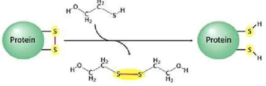
Fig. 1: Disulphide bond breakage.
Mild reductants and mild oxidants can lead to changes in protein conformation, that may alter the function of the protein. Mild reductants can break disulphide bonds (Fig. 1) and may lead to dissociation of parts of the protein chain(s) that are normally associated. Mild oxidants can cause the formation of disulphide bonds may lead to association of parts of the protein chain that are normally not associated. Stronger oxidising and reducing agents can change the nature of protein R groups most easily oxidised, if R groups next to sulphydryl groups are phenol (Tyr), hydroxyl (serine & threonine), amine (Lys, Arg, His), sulphide (Met)
Non-polar solvents disrupt hydrophobic interactions (association of non polar R groups) because non-polar R groups no longer associate, since they can now interact with the solvent. This leads to the dissociation of the non-polar R groups and results in unfolding of the protein chain.
1.6.3 Free Energy Derivation
Two basic approaches are present to study various contributions to protein stability: to study the protein stability as a function of environmental variables, such as temperature, denaturant concentration, pH, pressure, etc. with site- specific mutations in most cases. Second major approach is to study model systems where one attempts to mimic the folding process, with a system simpler than a protein so that it’s easier to interpret. Though the second approach has been considerably used, the first approach’s experimental data is proved to be more accurate and reliable for its use with theoretical models for
Depending on the environmental variables, different methods are employed to measure the free energy differences during protein denaturation. These methods are listed below:
(1) Differential Scanning Calorimetry (DSC) in which excess heat capacity has been used as a function of temperature.
(2) Fluorescence spectroscopy that uses intrinsic fluorescence of aromatic amino acids to monitor unfolding/refolding transitions induced by chemical denaturants, temperature, pH and pressure.
(3) UV spectroscopy that uses absorption of near UV (small shifts in wavelengths for folded and unfolded states) by amino acids to study folding/unfolding transitions.
(4) Circular Dichroism that measures the chirality of protein structures which can clearly distinguish between tertiary, secondary and unfolded structures.
In principle, apart from the widely used techniques described above, any physical technique that is capable of distinguishing the native and denatured states of a protein can be used to monitor the unfolding transition. Biological activity measurements, immunochemical techniques, hydrodynamic methods, such as viscosity, NMR, UV difference spectroscopy can all be used to follow unfolding.
1.6.4 ∆∆G and ∆∆GH2O
The native state of most naturally occurring proteins is only about 5-15 kcal/mol more stable than its unfolded conformations. By assuming the two state mechanism, only the folded and unfolded forms of the protein are present at significant concentrations and
fF + fU = 1 (5)
where fF and fU represent the fraction of the total protein in the folded and unfolded conformations, respectively. The observed values at any point of the transition curve is given by
y = yFfF + yUfU (6)
where y is any observable parameter chosen to follow unfolding, and yF and yU represent the values of y characteristic of the folded and unfolded protein. The values of yF and yU for any point in the transition region are obtained by extrapolation of the pre- and post-transition baselines, which is generally achieved by least squares analysis. Combining equations (5) and (6) yields
fU = (yF-y)/(yF-yU) (7)
The equilibrium constant KU, and the free energy change, ∆GU, for the folding/unfolding reaction can be calculated using
KU = fU/(1-fU) = fU/fF = (yF-y)/(y-yU) (8) and
∆GU = -RTlnKU = -RTln[(yF-y)/(y-yU)] (9) where R is the gas constant and T is the absolute temperature (K).
∆GUH2O, the free energy change in zero denaturant concentration is then calculated for the protein in equilibrium. To obtain an estimate of ∆GH2O from these studies, accurately measured values of the equilibrium constant, KU, are determined under denaturing conditions, and an attempt is made to extrapolate back to zero denaturant concentration. ∆GU is generally found to vary linearly with denaturant concentration. The simplest and at present most widely used model assumes that the linear dependence of ∆GU on denaturant concentration observed in the transition region continues to zero concentration of denaturant.
A least square analysis can be used to fit the data to an equation of the form:
∆GU = ∆GUH2O – m[denaturant] (10)
The value of m in this equation is a measure of the dependence of free energy on denaturant concentration. Apart from the linear expolation model, there are also other methods for analysing the denaturation curves (Wyman 1964; Inoue and Timasheff 1968).
After the point mutation, the difference in ∆GU and ∆GUH2O between mutant and wild type protein is then calculated (∆∆GU and ∆∆GUH2O). These values are often mentioned as ∆∆G and ∆∆GH2O in the literature.
1.6.5 Theoretical Background
Given the thermodynamic hypothesis, studies of protein folding (i.e. structure prediction, fold recognition, homology modelling and design) generally make use of some form of energy function. There are three different types of energy function that are in use.
The first is based on the true effective energy function, which can be obtained, in principle, from a fundamental analysis of the forces between the particles.
These are often known as physical effective energy functions (PEEF). PEEFs typically consist of a molecular mechanics energy function and a model for the effect of solvation on the free energy. Thus, PEEFs are approximations to the (unknown) true energy function.
The second is the empirical effective energy function (EEEF) and its approaches combine a physical description of the interactions with lessons learned from experiments. Good examples of such algorithms are the helix/coil transition algorithm AGADIR (Munoz and Serrano 1997; Lacroix et al. 1998) or the SPMP (Takano et al. 1999) method. The AGADIR algorithm is accurate at predicting the helical content of peptides in solution and has been used to design mutations that increase the thermostability of a protein through local interactions (Guerois et al. 2002). A limitation of this algorithm is that it can be applied only to α-helices and cannot take tertiary interactions into account.
Later, advanced variants of EEEFs were used by others for predicting changes in protein stability upon mutation.
The third is an energy function based on data derived from known protein structures (often statistics concerning pair contacts and surface area burial).
These are often known as statistical effective energy functions (SEEF). These are used initially by several researchers in the prediction of protein structure and stability.
1.7 Experimental Substitution Methods
Techniques for altering protein primary structure (sequence) using point mutations fall into three major categories: site-specific mutagenesis, random point mutations and shuffling. Numerous variants of each category exist, but the principles are general.
1.7.1 Site-Specific Mutagenesis
If a protein is produced in the laboratory by expression of its gene, point mutations can be readily introduced by site-directed mutagenesis, using the Polymerase Chain Reaction (PCR). Typically, the gene has already been cloned into a plasmid.
1.7.2 Random Mutations at Specified Positions
It is often desirable to investigate the effect of more than one amino acid on protein stability and function. If there is reason to believe a particular position was critical to folding, it’s essential to determine the substitutions at that position with increased stability. The most direct approach is to construct 19 site-directed mutations, each with the codon of a different amino acid at the centre of the primer, and measure the folding free energies of the wild type and all mutants. An alternative is to generate all possible mutants and screen for the most stable.
1.7.3 DNA Shuffling
DNA shuffling is used to carry out random mutations throughout the whole gene. The easiest way to construct random mutations is to do PCR with low- fidelity polymerase, which makes random mistakes during gene duplication.
Such error prone PCR can be combined with DNA shuffling so that diverse
sequences can be rapidly generated and selected. The method is intended to mimic recombination used by nature to generate biological diversity. A pool of identical or closely related sequences is fragmented randomly, and these fragments are reassembled into full-length genes via self-priming PCR and extension. This process is known as “assembly PCR” and yields crossovers between related sequences due to template switching. Such shuffling allows rapid combination of positive-acting mutations and simultaneously flushes out negative-acting mutations from the sequence pool. When coupled with effective selection, and applied iteratively, such that the output of one cycle is the input of the next cycle, DNA shuffling is an efficient process for directed molecular evolution. DNA shuffling is a recent invention, with the ability to sample much larger sequence space than other mutagenesis techniques. Most of its applications have been focused on discovering mutations leading to higher activities (e.g. resistance to antibiotics, higher enzymatic activities, and stronger cell fluorescence signal). Dramatic activity improvements have been achieved using DNA shuffling, and it will not be surprising if this technique uncovers mutated proteins that are much more stable than the wild type.
1.7.4 Protein Stability Assessment
There are several methods to measure protein stability as a function of an environmental perturbant. The most fundamental measures of protein stability involve temperature as the environmental variable. Differential scanning calorimetry (DSC), in which the excess heat capacity of a protein solution is determined as a function of temperature, can provide all the thermodynamic parameters that specify the stability of the protein as a function of temperature:
∆H, ∆S and ∆Cp. The ability to make single amino acid changes has provided another means by which investigators can probe the stabilisation of proteins.
The calculation free energy of unfolding was already explained in this chapter.
On the other hand, denaturants are also used to measure protein stability.
Spectroscopic (e.g., fluorescence spectroscopy, circular dichroism) techniques are also widely used to track the folding-unfolding transition, when these denaturants are used.