Master’s Thesis
Regional Variation of Health Care Expenditures in Austria
Name: Sophie Fößleitner
E-Mail: foessleitner@ihs.ac.at
Student ID-Number: 01108622
Supervisor: Univ. Prof. Marcel Bilger, PhD.
Second Supervisor: Dr. Mag. Anna-Theresa Renner, MSc.
Submitted on: 17.09.2020
WU Vienna University of Economics and Business
Health Economics and Policy Group
II Abstract
Over the last decades, the notion of widespread differences in health care expenditures
across regions has been firmly established and critically reviewed in the literature in
terms of their causes and consequences. In Austria, too, health care expenditures show
clear regional disparities. In 2016, there was regional variation in health care expendi-
tures at the district level which ranged from 50% below to 30% above the average of
1,844.15€ per inhabitant. When looking at the factors associated with the level of health
care expenditures per inhabitant, patient characteristics, especially demographic and
socioeconomic factors, can explain some of the regional disparities within the expendi-
tures of the Austrian health care system. This is in line with the theory which states that
in universal and publicly financed health care systems, such as the Austrian, regional
disparities will arise through the demand side. The analyses also find a positive relation-
ship between health care expenditures of different health care sectors and specialities,
namely between expenditures of the inpatient and the outpatient sector. The results have
implications for evidence-based health policies regarding inequalities as a good health
care system should deliver quality health services to all people when and where they
need them.
III TABLE OF CONTENTS
TABLE OF CONTENTS ... III LIST OF FIGURES ... IV LIST OF TABLES ... V LIST OF ABBREVIATIONS... VI
1 INTRODUCTION ... 1
2 THEORETICAL BACKGROUND ... 4
2.1 Theoretical causes of regional variation: determinants of health care expenditure ... 5
2.2 Empirical evidence of regional variation in health care expenditure ... 7
2.3 Relationship between health expenditures of different health care sectors and specialities ... 9
3 INSTITUTIONAL BACKGROUND ... 11
4 DATA AND METHODOLOGICAL APPROACH ... 13
4.1 Data ... 13
4.1.1 Health care expenditures ... 13
4.1.2 Covariates ... 17
4.2 Methodological approach ... 19
4.2.1 Regional variation of health care expenditures ... 19
4.2.2 Relationship between health expenditures in different health care sectors and specialities ... 22
5 RESULTS ... 24
5.1 Regional variation of health care expenditures ... 24
5.2 Relationship between health expenditures in different health care sectors and specialities ... 28
6 DISCUSSION ... 32
7 CONCLUSION ... 36
REFERENCE LIST ... XXXVII
APPENDIX ... XLIV
ACKNOWLEDGEMENTS ... XLVII
IV LIST OF FIGURES
Figure 1: Health expenditures as share of GDP (in %), Austria, 1988-2018 ... 1
Figure 2: Health expenditures as share of GDP (in %), EU countries, 2006 and 2016 ... 2
Figure 3: Histogram of district-level total expenditures per inhabitant in € ... 16
Figure 4: Boxplot of district-level total expenditures per inhabitant in € ... 16
Figure 5: Regional variation of total (health care) expenditures per inhabitant ... 24 Figure 6: Boxplot and histogram of district-level health expenditures per inhabitant in the
inpatient sector (in €) ... XLIV Figure 7: Boxplot and histogram of district-level health expenditures per inhabitant in the
outpatient sector (in €) ... XLIV
Figure 8: Boxplot and histogram of district-level health expenditures per inhabitant of GPs (in €) ... XLIV Figure 9: Boxplot and histogram of district-level health expenditures per inhabitant of
specialists (in €) ... XLV
Figure 10: Homoscedasticity – Model 1 ... XLV
Figure 11: Heteroscedasticity – Model 2 ... XLVI
Figure 12: Homoscedasticity – Model 3 ... XLVI
V LIST OF TABLES
Table 1: Descriptive statistics of health care expenditures ... 15
Table 2: Descriptive statistics of covariates ... 19
Table 3: Regression results – determinants of health care expenditures ... 26
Table 4: Results of correlation analysis ... 28
Table 5: SUR results – correlation of residuals ... 29
Table 6: SUR results – determinants of health care expenditures ... 31
Table 7: Results of regression diagnostics ... XLV
VI LIST OF ABBREVIATIONS
AIC Akaike information criterion
BIC Bayesian information criterion
BMSGPK Bundesministerium für Soziales, Gesundheit, Pflege und Konsumentenschutz, Federal Ministry of Social Affairs, Health, Care and Consumer Protection COPD chronic obstructive pulmonary diseases
CoV coefficient of variation
CT computer tomography
DRG diagnosis-related groups
DVSV Dachverband der österreichischen Sozialversicherungsträger, Main Association of Austrian Social Security Institutions e.g. exempli gratia, for example
EU European Union
GDP gross domestic product
ger. German
GP general practitioner
HRR hospital referral regions
ibid. ibidem, in the same place i.a. inter altri, among others i.e. id est, that is
LDF leistungsorientierte Diagnosefallgruppen, procedure-oriented diagnosis-related case groups
OECD Organisation for Economic Co-operation and Development
OLS ordinary least squares
ÖÄK Österreichische Ärztekammer, Austrian Medical Chamber
SD standard deviation
SUR seemingly unrelated regression
US United States of America
VIF variance inflator factor
WHO World Health Organisation
€ Euro
% per cent
1 1 INTRODUCTION
“A good health [care] system delivers quality services to all people when and where they need them.” (WHO, 2020)
The Austrian health care system is deemed to be one of the best in the world and access to medical services can be considered exemplary in international terms. As such, Aus- tria’s residents report the lowest level of unmet needs for medical care across the Euro- pean Union (EU) and virtually the whole population is covered by social health insur- ance while enjoying a broad benefit basket (Bachner et al., 2018). This, however, goes hand in hand with relatively high health expenditures which are also steadily increasing:
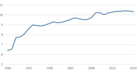
Over the last three decades, health expenditures as share of the gross domestic product (GDP) in Austria have risen from 6.40% in 1988 to 10.33% in 2018 (see Figure 1) (OECD, 2020).
Figure 1: Health expenditures as share of GDP (in %), Austria, 1988-2018
Data source: OECD (2020)
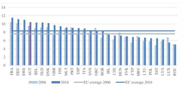
This phenomenon can also be observed for other countries of the European Union in recent years. As shown in Figure 2, health expenditures as share of GDP have increased in almost all EU countries from 2006 to 2016 (OECD, 2020).
1However, there are also some exceptions where expenditures have decreased, namely countries affected most by the austerity policies following the European debt crisis as well as Eastern European countries. Compared to the EU average, health expenditures as share of GDP in Austria
1
This time period was chosen in order to account for effects of the financial crisis of 2008/09 as well as the fact that health expenditures of the year 2016 will be the focus of this thesis.
5 6 7 8 9 10 11
1988 1993 1998 2003 2008 2013 2018
2
(9.5% in 2006 and 10.4% in 2016) have been well above the average of 7.6% in 2006 and 8.4% in 2016 (OECD, 2020).
Figure 2: Health expenditures as share of GDP (in %), EU countries, 2006 and 2016
Data source: OECD (2020)
The fact that health expenditures as a share of GDP have been increasing over recent years is an important observation since they have also been growing faster than the gross domestic product itself. Between 2006 and 2016, health expenditures in EU coun- tries have, on average, increased by 1.68% while the average growth rate of GDP was 1.11% (The World Bank, 2020). For Austria, this finding also holds as the average growth rate of current health expenditures was at 1.98% while that of GDP was at 1.28% (ibid.).
From a health economic perspective, these circumstances raise questions about the effi- ciency and the efficacy of a health care system. In general, rising expenditures could either increase the quality of health services as more resources are devoted to health or they could reduce the quality and the amount of medical services provided due to initial budget restrictions. In publicly financed systems, however, the latter argument seems to prevail which is why disproportionally increasing health expenditures can thus conflict with their aim to offer all insured the same (high) level of services, regardless of when and where they need them. Rising health expenditures are therefore also associated with a number of (in-)equality aspects as neither demographic, socioeconomic and social factors nor the place of residence of the insured should influence the quality, provision and utilisation of health care services. Within this framework, regional disparities play
0 2 4 6 8 10 12 14
F RA DEU S WE AUT BEL NLD DNK GBR F IN M LT P RT ES P ITA S VN GRC BGR IRL CZE HUN S VK CYP HRV LTU P OL ES T LVA LUX ROU
2006 2016 EU average 2006 EU average 2016
3
an important role as the presence of such regional variation in health care expenditures warrant specific health policies which can support a needs-based and equal care for all insured. Research shows that regional variation in health care expenditures can be due to supply-driven or demand-side factors with the latter being predominant in universal and publicly funded health care systems (e.g. de Vries et al., 2018; Lavergne et al., 2016; Skinner, 2012).
From a health policy perspective, disproportionally increasing health expenditures also constitute a challenge if medical services are not provided on the basis of medical need.
One way to establish whether the provision of services is needs-based is to look at the relationship between different health care sectors and the associated expenditures as a higher medical need will lead to higher health expenditures in all care sectors in a pub- licly-funded health care system.
The aim of this thesis is therefore twofold: First, it will be established whether there is regional variation in health care expenditures in Austria. If so, the determinants of health expenditures will also be studied. Second, it will be examined whether there is a relationship between health care expenditures of different health care sectors and speci- alities such that their levels influence each other. If so, it will also be studied whether the determinants of health expenditures in different care sectors and specialities differ from each other. These analyses will be carried out for claims data of selected social health insurance funds for the year 2016.
The ensuing hypotheses are that there is regional variation in health care expenditures in Austria which can be associated with heterogeneity in patient characteristics. Regional disparities will therefore be related to demand-side factors as the Austrian health care system is publicly funded. Furthermore, it is expected that there is a relationship be- tween health expenditures of different health care sectors and specialities as higher medical needs will lead to higher expenditures in all care sectors.
The following thesis is structured thusly: Section 2 provides an overview of the litera-
ture concerning the determinants of health care expenditures as well as the relationship
between expenditures of different health care sectors while section 3 reviews the Aus-
trian health care system. Section 4 introduces the data basis and the variables used in the
analysis as well as discusses the applied research methodologies. Section 5 then de-
scribes the results while sections 6 and 7 discuss and conclude.
4 2 THEORETICAL BACKGROUND
Over the last decades, the notion of widespread differences in health care expenditures across regions has been firmly established and critically reviewed in the literature. Most of the existing research comes from the United States (US) and centres around the sem- inal paper of Wennberg and Gittelsohn (1973) as well as follow-up studies of the Medi- care
2population (i.a. Corallo et al., 2014; Cutler et al., 2019; Fisher et al., 2003a, 2003b, 2004; Paul-Shaheen et al., 1987; Wennberg, 2002; Wennberg et al., 2002). Recently, however, the analysis of marked variations in the health care systems has also been car- ried out in other countries, including Canada (Lavergne et al., 2016), Germany (e.g.
Göpffarth, Kopetsch, & Schmitz, 2016), Italy (Giannoni & Hitiris, 2002), the Nether- lands (de Vries et al., 2018), Spain (Prieto & Lago-Peñas, 2012) and Switzerland (Reich, Weins, Schusterschitz, & Thöni, 2012). Due to the different structure and the size of the welfare state of the respective health care systems, US-based results regard- ing the causes and consequences of regional variations cannot be directly applied to the Austrian case, despite offering possible explanatory approaches, while those from the other aforementioned OECD countries are more suited to do so. For Austria, there exists only very little empirical evidence regarding small area variations in health care spend- ing so far. One recently published study (Hofmarcher & Molnárová, 2018) however states that there are striking differences in health care spending as well as health status between the nine Austrian provinces even though this is not examined in more detail.
Given the steady increase in health care expenditures over recent years, researchers have also looked into the relationship between health expenditures of different health care sectors and specialities (e.g. Adhikari, 2012; Atella and Deb, 2008; Büyükdurmus et al., 2017; Fortney et al., 2005; Kopetsch, 2007). This relationship can either be posi- tive, negative or non-existent and may imply necessary structural reforms of the health care system (Fortney et al., 2005). For Austria, there is no empirical evidence of the interdependence between health expenditures of different care sectors so far.
The following literature survey therefore discusses the theoretical causes of regional variation (section 2.1) as well as providing empirical evidence of regional disparities in
2
Medicare is a federal government program in the US which provides health care coverage (health insur-
ance) for people over the age of 65 as well as for younger people with end-stage renal diseases and
those receiving disability benefits. Benefits include inpatient as well as outpatient (medical) coverage
with optional prescription drug coverage. (Medicare Interactive, 2019)
5
health expenditures (section 2.1). Finally, a quick overview of the relationship between the health expenditures of different health care sectors and specialities is given (section 2.3).
2.1 Theoretical causes of regional variation: determinants of health care expenditure
Economic theory suggests that there are two potential causes of regional variations in
health care: demand-side and supply-driven factors. Demand-side factors reflect medi-
cal need and patient preferences for care as well as access barriers to health care (Skin-
ner, 2012). This also includes patient heterogeneity between regions in terms of income,
age, gender, education, health status and the prevalence of (chronic) diseases and multi-
morbidities (de Vries et al., 2018; Skinner, 2012). Hence if there is heterogeneity on the
demand side because patients are sicker, prefer specific treatments or do not have access
to specific medical services, regions will also vary with respect to health care expendi-
tures. Crucial within this perspective is the so-called social gradient which describes the
phenomenon whereby people who are less advantaged in terms of their socioeconomic
position have worse health outcomes than those who are more advantaged and are thus
also in need for more health care, causing higher expenditures (Donkin, 2014). Studies
have therefore examined how strongly socioeconomic inequalities influence health out-
comes such as life expectancy and, as a consequence, health care expenditures of people
living in different regions (Kibele, Klüsener, & Scholz, 2016; Sundmacher, Kimmerle,
Latzitis, & Busse, 2011). In the United States, for instance, geographic disparities in life
expectancy are large and amounted to as much as 20 years in 2014 (Dwyer-Lindgren et
al., 2017). The fact that 74% of this variation can be explained by a combination of so-
cioeconomic (e.g. income, educational attainment or occupation) and race/ethnicity fac-
tors, behavioural and metabolic risk factors (e.g. prevalence of diabetes mellitus, hyper-
tension or obesity) as well as health care factors points to the importance of non-
medical determinants as predictors of mortality and therefore also the level of health
expenditures (Dwyer-Lindgren et al., 2017; Lavergne et al., 2016). This branch of re-
search is hence closely related to the analysis of health inequalities, i.e. avoidable dif-
ferences in health between groups of people within and between countries and their so-
cieties, but with a spatial component (World Health Organization, 2019).
6
On the supply side, factors such as provider financial incentives, capacity constraints, physician beliefs and practice norms play an important role (Skinner, 2012). One fea- ture within this context is the so-called supplier-induced demand where a health care provider shifts a patient’s demand curve beyond the level of care that the fully informed patient would otherwise want, i.e. doctors and hospitals create their own demand by carrying out too many medically unnecessary treatments in order to maximize their profits (Cutler et al., 2019; J. E. Wennberg, Barnes, & Zubkoff, 1982). If the variation in supply-side factors is spatially correlated, for example if physicians with more inten- sive treatment styles hire other physicians with similar beliefs and practice norms, the resulting regional differences on the provider side could explain regional variations in health care expenditure (Cutler et al., 2019).
Apart from that, system factors such as (insurance) regulation, price setting or payment, and, in publicly-funded systems, the general economic conditions also influence the dynamics of demand and supply (de Vries et al., 2018; Eibich & Ziebarth, 2015). While demand factors are generally considered justifiable causes of variation in health care spending, regional variation as a result of supply factors is deemed to be undesirable as regional variation in health care spending not caused by differences in medical need is said to indicate inefficiency (de Vries et al., 2018). The latter especially holds if higher health care expenditures are not associated with better health outcomes (Baicker &
Chandra, 2004; Corallo et al., 2014; Fisher et al., 2003a, 2003b; Lavergne et al., 2016;
Sirovich, Gottlieb, Welch, & Fisher, 2006; J. Wennberg & Gittelsohn, 1973).
Econometric models try to parse out whether demand, supply or other factors are the most important determinants in explaining regional variations in health care expendi- ture; the results differ depending on which countries are examined. However, caution should be exercised when interpreting the corresponding results as one very common problem within these analyses concerns the issue of reverse causality between health expenditures and health outcomes (Göpffarth et al., 2016; Skinner, 2012). In general, reverse causality refers to a direction of cause-and-effect contrary to a common pre- sumption, i.e. if two variables X and Y are associated, it might be the case that Y is causing changes in X instead of the other, expected, way around (Woolridge, 2014).
Applying this conjuncture to health expenditures and health outcomes, causality can
therefore work in both directions: A high poor health outcome can either be the result of
7
high expenditures if their level is demand-side driven (“higher needs lead to poor out- comes and higher expenditures”) or of low expenditures if the needs of patients are not met (“undetected needs lead to poor outcomes and lower expenditures as patients are not treated”). The interpretation of the results thus depends on the specific health care system and yields rather associative than causal conclusions (see section 6).
2.2 Empirical evidence of regional variation in health care expenditure
For decades, researchers have documented marked variation in health care spending across and within regions all over the world (i.a. Fisher et al., 2003a, 2003b; Göpffarth et al., 2016; Lavergne et al., 2016; Reich et al., 2012; Skinner, 2012; Wennberg and Gittelsohn, 1973; Zhang et al., 2012).
For the United States, research has shown that Medicare spending varies more than two- fold across hospital referral regions 3 (HRRs) as well as from state to state and from one hospital to another (The Dartmouth Institute for Health Policy & Clinical Practice, 2019). In 2016, price-adjusted Medicare reimbursements among the 306 HRRs in the US varied from about $7,400 per enrollee in the lowest spending region to more than
$13,000 in the highest spending region (ibid.). Most of this variation is due to supply- side factors, especially physician organizational factors and physician beliefs about treatment (Cutler et al., 2019). In this context, there is also a profound body of empirical evidence documenting that these marked variations in health care expenditures are the result of inefficiencies as regions with higher spending and service use do not automati- cally display better health outcomes (Baicker & Chandra, 2004; Corallo et al., 2014;
Fisher et al., 2003a, 2003b; Lavergne et al., 2016; Sirovich et al., 2006; J. Wennberg &
Gittelsohn, 1973). Studies in line with this argumentation find that more than 50% of the variation in Medicare spending across regions cannot be explained, thus indicating inefficiencies (Fisher et al., 2003a, 2003b; Göpffarth, 2011; Institute of Medicine (IOM), 2013; Skinner, 2012). Over the recent years, however, this view has been criti- cally reviewed (e.g. Sheiner, 2014; Song et al., 2010; Zuckerman et al., 2010). The main criticism relates to the fact that this conclusion is very often based on a correlation ra-
3
Hospital referral regions (HRRs) represent regional health care markets for tertiary medical care that
generally require a major referral centre, i.e. a hospital where patients are referred to for major cardio-
vascular surgical procedures and for neurosurgery. (The Dartmouth Institute for Health Policy & Clin-
ical Practice, 2019; Zhang, Baik, Fendrick, & Baicker, 2012)
8
ther than a causal relationship (Eibich & Ziebarth, 2014; McWilliams et al., 2014). This opinion has been supported by Sheiner (2014) who claims that the relationship between spending and outcomes is not the result of inefficiencies but rather of omitted variables on the demand side which biases the conclusion.
The results for other OECD countries contrast quite strongly with studies from the US as there is only weak evidence for inefficiencies as a cause for regional variation even though there are pronounced regional disparities within the respective health care sys- tems (Göpffarth et al., 2016). This might relate to the fact that many of these health care systems differ quite substantially from the US as prices, insurance coverage and the degree of cost sharing are invariant across the region, the legal context for medical prac- tice is constant as well and results represent the entire population, including all age groups, fully insured (Lavergne et al., 2016). Therefore, many of the mechanisms driv- ing regional variation observed in the United States are not relevant for other OECD countries, thus leading to very different results (Lavergne et al., 2016; Manning, Norton,
& Wilk, 2012). The findings for these countries hence indicate that regional variation in health care expenditures is largely explained by demand-side factors, especially patient characteristics (de Vries et al., 2018; Eibich & Ziebarth, 2014; Giannoni & Hitiris, 2002; Göpffarth et al., 2016; Lavergne et al., 2016). In Canada, for example, unadjusted spending in the most expensive health region was 50% higher than in the least expen- sive (Lavergne et al., 2016). However, after adjustment for patient characteristics, in- cluding age, sex, recorded diagnoses and the residence of patients, only very little unex- plained variation among health regions remains (ibid.). For Germany (Eibich &
Ziebarth, 2014, 2015; Göpffarth, 2011, 2013, 2015; Göpffarth et al., 2016; Nolting,
2018), the Netherlands (de Vries et al., 2018) and Italy (Giannoni & Hitiris, 2002) simi-
lar conclusions can be made. This result is consistent with the conjuncture that in coun-
tries with centrally-provided and publicly-funded health care, a person’s demand for
care is not limited by supply factors such as price, private budgetary considerations or
the ability to pay which is why regional variations should arise through differences on
the demand-side (Pauly, 1986).
9
2.3 Relationship between health expenditures of different health care sectors and specialities
Generally speaking, different health care sectors or specialities and their corresponding health expenditures can either have a positive, a negative or no relationship at all. If sectors or specialities are positively related, health services and their expenditures are called complements as they are mutually dependent on each other. As such complemen- tary health services are those that tend to be delivered or consumed together and there- fore rise expenditures in all involved health care sectors (Fortney et al., 2005). A posi- tive relationship between health expenditures of different sectors or specialities there- fore implies, among other things, that patient characteristics and especially medical needs are important determinants of health care expenditures
4. Substitutes, by contrast, are those health services and corresponding expenditures which exhibit a negative rela- tionship between them and can be delivered or consumed instead of each other which rises expenditures in one health sector and decreases them in another.
The existing literature on interdependences between health expenditures of different health care sectors or specialities is not very extensive and does not provide a clear pic- ture of the relationship between care sectors. The latter could be due to the fact that in many countries the health care system is structured in a way that access to medical ser- vices is restricted by law which is enforced through a so-called Gatekeeper model (Büyükdurmus et al., 2017). In these models, the general practitioner (GP) has the task of piloting patients through the health care system, thereby authorising treatment by specialists in the outpatient sector or referring them to the inpatient sector (ibid.). This system therefore warrants a purely complementary relationship between different health care sectors and specialities as secondary care (specialists, inpatient services) can, in most cases, only be consumed after using primary care at the GP thus increasing health expenditures in all involved care sectors (ibid.). In health care systems where there is no such model in place, however, there is clear heterogeneity in the interdependences be- tween different sectors. As such, the direction of the relationship strongly depends on
4
There are also other possible mechanisms which warrant a positive relationship between health expendi-
tures of different care sectors and specialities. These include regional clustering due to similar physi-
cian beliefs or spill-over effects in practice styles, e.g. if doctors work both in the in- and the outpa-
tient sector. In both cases, health expenditures of different providers and sectors may develop in the
same direction. However, these mechanisms are rather more relevant in non-public health care sys-
tems which is why they are not considered further in this analysis of a publicly funded system.
10
the medical speciality as well as on the specific setting and methods of the respective study in a way that some find a complementary relationship while others find a substitu- tive one for the same specific situation (Büyükdurmus et al., 2017).
Studies have been carried out, among others, for Germany (Büyükdurmus et al., 2017;
Kopetsch, 2007), Italy (Atella & Deb, 2008) or the United States (i.a. Fortney et al., 2005) and, as mentioned before, report contradictory findings. However, they all estab- lish a relationship between health expenditures of different sectors or specialities.
Best reviewed in the literature is the relationship between inpatient, outpatient and/or primary care services and their corresponding health expenditures (e.g. Adhikari, 2012;
Atella and Deb, 2008; Büyükdurmus et al., 2017; Fortney et al., 2005; Kopetsch, 2007).
Theory suggests that there are a number of possible mechanisms by which outpatient or primary care services can be a complement or substitute with inpatient services. Mecha- nisms for complementation are the utilisation of services that are truly supplemental or ancillary to each other (e.g. diagnostic laboratory tests), the detection of illnesses that cannot appropriately be treated in one health care sector, such as cancer, and the identi- fication of acute episodes which require further treatment in another speciality or care sector like angina pectoris (Fortney et al., 2005). Substitution mechanisms, on the other hand, are the prevention, early detection or delay of illnesses in one health care sector which may avert treatment in another speciality or sector (Donaldson, Yordy, Lohr, &
Vanselow, 1996; Starfield, 1994). However, there is also the possibility that substitution effects arise due to structural inefficiencies of health care system which lead patients to consume medical services not based on their medical need but rather due to misinfor- mation (“use of the ‘wrong’ health care provider”) or the distance to the nearest health care provider (Fortney et al., 2005; Göpffarth et al., 2016).
As mentioned above, there exists only limited evidence on small area regional variation
of health care expenditures in Austria. This thesis therefore contributes to the literature
in providing a first overview of eventual regional variations in health expenditures as
well as in establishing potential determinants of these expenditures. In addition, it also
adds in ascertaining an interdependence between health expenditures of different sectors
or specialities as no such detailed examination has been carried out for Austria so far.
11 3 INSTITUTIONAL BACKGROUND
5As evidence suggests (see section 2.1), the institutional background plays an important role for the causes of regional variation in health care expenditures. Therefore, the Aus- trian health care system and its structure will be shortly reviewed in the following.
The Austrian health care system is based on the principles of solidarity, affordability and universality, with the most important guideline being that access to high-quality health care is provided equally to everyone in need regardless of the person’s age, gen- der, origin, social status and income. It can thus be categorized as an universal health care system with health care expenditures as a share of GDP amounting to 10.3% in 2018, which is considerably higher than the EU average of 8.3% (OECD, 2020). More than 75% of total health care expenditure is financed from public sources, about 18% is made out-of-pocket by the patients and the rest is financed via voluntary private health insurance which plays only a minor role in the system. In total, public health expendi- tures constitute 16% of government expenses which are financed by a mix of general tax revenues (40%) and compulsory social health insurance contributions (60%) (OECD, 2019).
Health care is based on a social insurance model founded on compulsory insurance so that 99.9% of the population in Austria are covered. All of the insured people have a legal right to services, which are financed via contributions on the basis of solidarity, and they enjoy a broad benefit basket as well as good access to health care. The level of contributions in the social insurance system is independent of the individual health risk of the insured and is rather an income-related amount. For the majority of those covered by health insurance, the contribution is 7.65% of their gross wage, up to a maximum level of gross income of 5,130€ in 2018. In total, contributions are paid in almost equal parts by the employer and the employee. At the moment, there are five social insurance funds
6which are responsible for health, pension and accident insurance; enrolment in one of the funds takes place according to the occupational status as well as the place where people live or work. Even though health insurance is thus generally linked to employment, coverage is extended to co-insured persons, such as spouses and depend-
5
If not stated otherwise, this section is based on Bachner et al., (2018) and Federal Ministry for Labour, Social Affairs, Health and Consumer Protection (2019).
6
Up to January 1
st2020, there were 21 social insurance funds – 19 of which were social health insurance
funds - which were reduced to five during the latest structural reform.
12
ents, pensioners, students, people with disabilities and those receiving unemployment benefits.
There are a large range of health care services available to the population and as such, Austria’s residents report the lowest level of unmet needs for medical care across Eu- rope (OECD/EU, 2018). Provision of health services in Austria is characterized by rela- tively unrestricted access to all levels of care including general practitioners (GPs), spe- cialists and hospitals, i.e. there is a free choice of doctors and no Gatekeeper model in place. This implies that, apart from a few exemptions (e.g. CT examination), there is no obligation to obtain the consent of the health insurance institution before using the ser- vices of contracted doctors, outpatient clinics and general practitioners. In the outpatient sector, patients also have the choice between contracted physicians (45%) and those without contract (55%), for using the latter one exists the possibility of partial reim- bursement from the social health insurance funds. The Austrian health care system has, however, a strong focus on inpatient care which becomes visible by a high hospital uti- lisation given by, for example, the hospital bed density for which Austria shows the second highest number compared to other EU countries (OECD/EU, 2018).
In terms of organisation and governance, the Austrian health care system is quite com-
plex and fragmented: Not only are the responsibilities shared between the federal and
the regional (Bundesländer) level, but some of them are also delegated to self-governing
bodies such as social insurance and professional bodies of health service providers. This
in turn leads to a mixed health care financing between the state (federal and regional
level) and the social health insurance funds who contribute to different parts of the
budget. Several reform attempts over the recent years have aimed at improving coopera-
tion and coordination in the health care system, but some crucial challenges still remain.
13
4 DATA AND METHODOLOGICAL APPROACH
In the following, the database (section 4.1) and the methodological approach (section 4.2) used for the analysis of the regional variation of health care expenditures in Austria as well as for the examination of the relationship between health expenditures of differ- ent health care sectors and specialities is described in detail.
4.1 Data
The empirical analysis of this thesis is performed for the year 2016 and expands on data from four different sources: Firstly, and most importantly, it uses claims data from the Main Association of Austrian Social Security Institutions (ger. Dachverband der öster- reichischen Sozialversicherungsträger, DVSV) for the key variable “health care expen- ditures”. Secondly, it draws upon administrative data from the Federal Ministry of So- cial Affairs, Health, Care and Consumer Protection (ger. Bundesministerium für Sozia- les, Gesundheit, Pflege und Konsumentenschutz, BMSGPK), the Austrian statistical bu- reau (ger. Statistik Austria) and the Austrian Medical Chamber (ger. Österreichische Ärztekammer, ÖÄK) for the covariates of the empirical analysis. All datasets are merged at district level which is also the unit of observation. As of 2020, there were 116 dis- tricts in Austria which is therefore the maximum number of observations in the sample.
In order to ensure comparability at district level, the statistical examination of health care expenditures is carried out per inhabitant according to the so-called residence prin- ciple. This means that the indicators are evaluated by source, i.e. on the basis of the res- idence of the beneficiaries and not on the location of the service providers. All health care expenditures are district-level average values, for nationwide representations, the size of the districts is also taken into account in order to avoid demographically induced distortions.
4.1.1 Health care expenditures
The analysis of the regional variation of health care expenditures as well as the exami- nation of the relationship between health care expenditures of different health care sec- tors takes both the inpatient as well as the outpatient sector into account.
For the inpatient sector, health care expenditures are calculated by drawing on the diag-
nosis-related groups (DRG) system which is a nationwide uniform model for the billing
14
of inpatient hospital stays. As such, inpatient hospital stays are grouped into procedure- oriented diagnosis-related case flat rates (LDFs) on the basis of the data collected in hospitals (Hagenbichler, 2010). For the analysis, the sum of LDFs in each district are provided by the Main Association of Austrian Social Security Institutions and expendi- tures for the inpatient sector were calculated retrospectively using a point value
7which reflects the public health care expenditures.
For the outpatient sector, claims data from the Main Association of Austrian Social Se- curity Institutions are used to examine health care expenditures. In doing so, the mone- tarily quantified value of all medical and similar services which is billed with and paid out by the social health insurance funds are considered. The figures are aggregated at the district level and the study cohort includes health services provided to patients of the 13 biggest social health insurance funds in the year 2016
8. Health care expenditures in the outpatient sector include expenditures for medical services (general practitioners, specialists, other health care providers and dentists), medicines, aids and appliances (ger. Heilbehelfe und Hilfsmittel) as well as for transport. Specialists include doctors of all specialties except general and dental medicine, other health care providers encom- pass health professionals such as therapists or rehabilitation facilities.
The analysis of the regional variation of health care expenditures draws upon the varia- ble "total expenditure" which consists of expenditures in the inpatient and outpatient sectors. For the examination of the relationship between health care expenditures of different care sectors, however, health care expenditures of the different sectors (inpa- tient and outpatient sector) and specialities (general practitioners and specialists) were evaluated separately. Table 1 presents descriptive statistics of the health care expendi- tures in the sample. Note that the various sectors and specialities cannot be summed up as the data query considers every patient only once, e.g. in order to be taken into ac- count for the variable “total expenditure”, one has to take up services in either the inpa-
7
In general, the point value describes inpatient expenditures, while the implicit value adjusts these ex- penditures for private expenditures and therefore reflects the real public expenditures. This implicit point value was provided by the Institute for Advanced Studies (IHS). In 2016, the implicit point val- ue was 1.34, i.e. one LDF corresponded to 1.34€.
8
As of 2016, there were 19 social health insurance funds, the 13 included in the analysis are the nine
regional health insurance funds (ger. Gebietskrankenkassen, GKK), the public servants social insur-
ance fund (ger. Versicherungsanstalt öffentlich Bediensteter, BVA), the social insurance fund for
commerce and industry (ger. Sozialversicherung der gewerblichen Wirtschaft, SVA) as well as for
farmers (ger. Sozialversicherungsanstalt der Bauern, SVB) and the railways social insurance fund
(ger. Versicherungsanstalt für Eisenbahnen und Bergbau, VAEB).
15
tient or the outpatient sector or in both. However, if a patient is included in the variable
“total expenditures”, this does not imply that he/she will also be included in the other expenditure variables as here it does depend on the specific sector of utilisation. It is for this reason that the variables “inpatient sector” and “outpatient sector” cannot be summed up to the variable “total expenditures” even though they contain, in theory, the same information. The same applies to the variable “outpatient sector” or the variables
“general practitioners” and “specialists”, respectively.
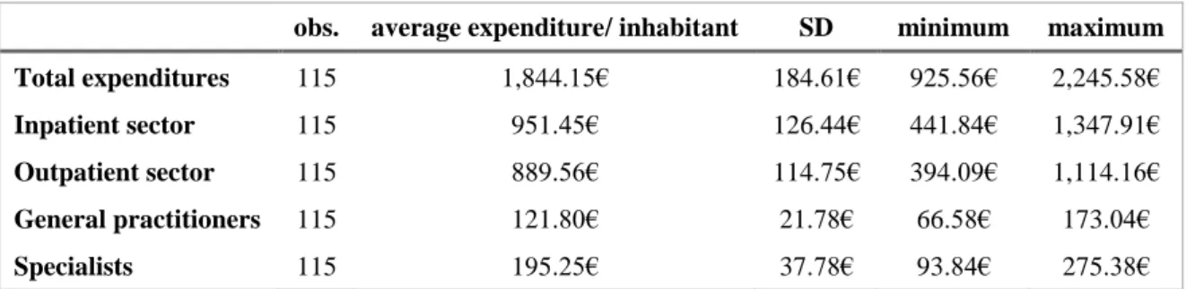
Table 1: Descriptive statistics of health care expenditures
obs. average expenditure/ inhabitant SD minimum maximum
Total expenditures 115 1,844.15€ 184.61€ 925.56€ 2,245.58€
Inpatient sector 115 951.45€ 126.44€ 441.84€ 1,347.91€
Outpatient sector 115 889.56€ 114.75€ 394.09€ 1,114.16€
General practitioners 115 121.80€ 21.78€ 66.58€ 173.04€
Specialists 115 195.25€ 37.78€ 93.84€ 275.38€
Note: obs.= observations, SD= standard deviation
Data source: Main Association of Austrian Social Security Institutions
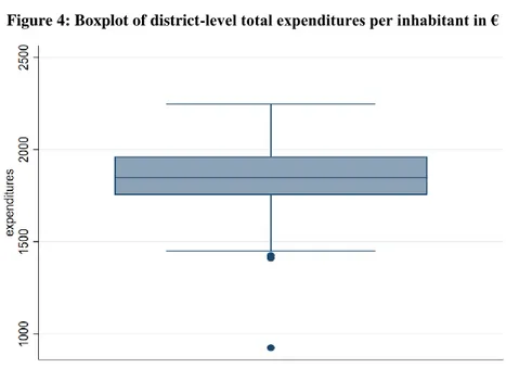
In 2016, total health care expenditures reached a total of 16,044,930,265.54€ and there were 8,700,471 Austrian inhabitants. The average total expenditure per district amount- ed to 1,844.15€ per inhabitant whereby it ranged from 925.56€ to 2,245.58€ (see Table 1). This distribution can also be seen in Figure 3 which displays the district-level fre- quency of average total expenditures per inhabitant by means of a histogram as well as in Figure 4 which shows a boxplot of average total expenditures per inhabitant at the district level.
99
The histograms and boxplots of the other variables (inpatient sector, outpatient sector, GPs and special-
ists) can be found in the appendix.
16
Data source: Main Association of Austrian Social Security Institutions
Data source: Main Association of Austrian Social Security Institutions
As can be seen from both figures above, there is one main outlier within the sample, i.e.
there is one district where average total expenditures per inhabitant were a lot lower compared to the other districts in 2016. However, due to the fact that it cannot be ascer- tained whether this is due to a systematic error in the data or due to other reasons, the outlier was not removed from the sample.
Table 1 also indicates that, compared with the outpatient sector, health care expendi- tures at the district level in the inpatient sector were slightly higher and averaged 951.45€ per inhabitant in 2016 while those in the outpatient sector reached 889.56€.
Looking solely at general practitioners and specialists in the outpatient sector, it be-
Figure 3: Histogram of district-level total expenditures per inhabitant in €
Figure 4: Boxplot of district-level total expenditures per inhabitant in €
17
comes apparent that district-level average health care expenditures were accordingly lower and amounted to 121.80€ per inhabitant for GPs and 195.25€ per inhabitant for specialists in 2016.
4.1.2 Covariates
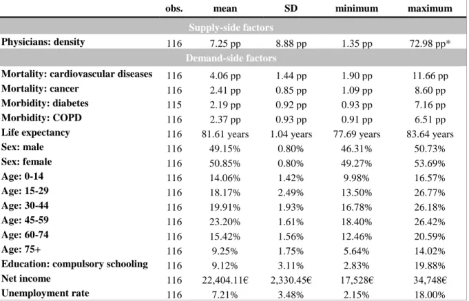
The analysis also draws upon further variables which are likely to be determinants of health care expenditures in Austria and which are therefore also used in the empirical analysis. In line with the theory (see for example Göpffarth et al., 2016), these covari- ates include supply-side as well as demand-side factors. As such, information about the supply of physicians for the supply side and data on selected health outcomes as well as socioeconomic and demographic variables are considered for the demand side.
Information about the supply of physicians is made available by the Austrian Medical Chamber and consists of the density of physicians per 1,000 inhabitants. Thereby, both the inpatient and the outpatient sector as well as all specialities, with the exception of dental medicine, are considered.
Data on selected health outcomes is provided by the Federal Ministry of Social Affairs, Health, Care and Consumer Protection as well as the Austrian statistical bureau. The health outcomes are selected on the basis of their significance for the morbidity and mortality burden in Austria so that both chronic diseases and the two most frequent causes of death - cardiovascular diseases and cancer - are taken into account (Statistik Austria, 2020). As a result, the number of deaths due to cardiovascular diseases and malignant neoplasms (cancer) on the one hand and the number of hospital stays with the main diagnoses "diabetes" and “chronic obstructive pulmonary diseases (COPD)” as approximate values for chronic diseases on the other hand are considered. All health outcomes are extrapolated to 1,000 inhabitants.
Socioeconomic and demographic variables are supplied by the Austrian statistical bu-
reau and include general life expectancy, age and gender distribution, education level
and net annual income of the population as well as the unemployment rate in the dis-
trict. For the age distribution, the respective shares of six different age groups (0-14, 15-
29, 30-44, 45-59, 60-74, 75+) were used, for the gender distribution the shares of wom-
en and men respectively. The level of education is approximated by the share of persons
with only compulsory schooling; a district average is used for the net annual income.
18
The descriptive analysis of the covariates, depicted in Table 2, yields the following re- sults: In 2016, the average density of physicians was 7.25 doctors per 1,000 inhabitants.
On the demand side, the average mortality for cardiovascular diseases was 4.06 persons per 1,000 inhabitants while the one for cancer was lower with 2.41 persons. The average morbidity of the population, which is being approximated by the number of hospital stays with the most prominent chronic diseases being the main diagnoses, was 2.19 per- sons per 1,000 inhabitants for diabetes and 2.37 persons for COPD. Looking at demo- graphic and socioeconomic variables, it becomes apparent that, in 2016, on average, the life expectancy was 81.61 years, there were slightly more women than men (50.85% vs.
49.15%), the biggest age group consisted of people aged 45 to 59 years, 9.12% of the population finished compulsory schooling only, the annual net income was 22,404.11€
and the unemployment rate was 7.12%. A more detailed summary of the descriptive statistics of the covariates can be found in Table 2 below
10.
10
Note that the means presented in Table 2 refer to unweighted average values, i.e., contrary to the health
care expenditures, the size of the individual districts is not accounted for.
19
Table 2: Descriptive statistics of covariates
obs. mean SD minimum maximum
Supply-side factors
Physicians: density 116 7.25 pp 8.88 pp 1.35 pp 72.98 pp*
Demand-side factors
Mortality: cardiovascular diseases 116 4.06 pp 1.44 pp 1.90 pp 11.66 pp
Mortality: cancer 116 2.41 pp 0.85 pp 1.09 pp 8.60 pp
Morbidity: diabetes 115 2.19 pp 0.92 pp 0.93 pp 7.16 pp
Morbidity: COPD 116 2.37 pp 0.93 pp 0.91 pp 6.51 pp
Life expectancy 116 81.61 years 1.04 years 77.69 years 83.64 years
Sex: male 116 49.15% 0.80% 46.31% 50.73%
Sex: female 116 50.85% 0.80% 49.27% 53.69%
Age: 0-14 116 14.06% 1.42% 9.98% 16.57%
Age: 15-29 116 18.17% 2.49% 13.50% 26.77%
Age: 30-44 116 19.91% 1.93% 16.78% 26.18%
Age: 45-59 116 23.20% 1.61% 18.40% 26.42%
Age: 60-74 116 15.42% 1.56% 12.46% 20.59%
Age: 75+ 116 9.25% 1.75% 5.64% 14.02%
Education: compulsory schooling 116 9.12% 3.11% 2.83% 19.88%
Net income 116 22,404.11€ 2,330.45€ 17,528€ 34,748€
Unemployment rate 116 7.21% 3.48% 2.15% 18.00%
Note: obs.= observations, SD= standard deviation, pp= persons (physicians) per 1,000 inhabitants
* In this case. the maximum density of physicians per 1,000 inhabitants can be considered as an outlier as the corresponding district is the one where Austria’s biggest hospital, the Vienna General Hospital (ger.
Allgemeines Krankenhaus Wien, AKH), is located. However, it is still included in the analysis in order to get the whole picture.
Data source: DVSV, BMSGPK, ÖÄK and Statistik Austria
4.2 Methodological approach
The empirical analysis is divided into two parts: While part one focuses on the regional variation of total health care expenditures in Austria, part two emphasises the relation- ship between health expenditures in different health care sectors and specialities as well as their determinants. Each part uses a different methodological approach which is de- scribed in detail in the following.
4.2.1 Regional variation of health care expenditures
The statistical examination in part one is carried out using a two-step approach. At first,
the data is thoroughly descriptively analysed in order to establish whether there is re-
gional variation in total health care expenditures in Austria at all. This is done, on the
one hand, by looking at the deviation from the mean and, on the other hand, by calculat-
ing the coefficient of variation. The deviation from the mean is presented in percentages
20
per district while the coefficient of variation (CoV) is calculated as ratio of the standard deviation and the mean (Woolridge, 2014). As a result, it can be shown that there is regional variation at the district level if the deviation from the mean is unequal to zero and if the CoV is greater than zero.
Granted that the analysis in the first step reveals that there is regional variation in total health care expenditures in Austria, the determinants of these heath care expenditures will be examined in more detail as a second step. To explore the per-inhabitant health expenditures per district, a multiple linear regression model
11in which the total expendi- tures are regressed on different control variables will be estimated. The unit of observa- tion is the district (Ν = 115) and the following model is used:
𝑦 𝑖 = 𝛽 0 + 𝛽 1 𝑋 1𝑖 + 𝛽 2 𝑋 2𝑖 + 𝜀 𝑖 (1) where
The regression analysis consists of two estimations whereby a restricted form of the model as well as the full model will be estimated. As such, the restricted-form model accommodates the supply of physicians for the supply side as well as the morbidity and mortality of the population for the demand side while the full model expands on these covariates and also includes demographic and socioeconomic characteristics of the pop- ulation as demand-side factors. This approach is used in order to disentangle the effect of medical need on health expenditures due to the disease burden on the one hand and patient characteristics on the other hand.
Following the model estimations, regression diagnostics will be carried out in order to ascertain whether the results are unbiased and consistent as well as to determine the goodness of fit. In doing so, standard testing for common inefficiencies, namely hetero- scedasticity and multicollinearity, as well as for model specification will be applied. In econometrics, heteroscedasticity means that the variance of the error term, given the explanatory variables, is not constant which renders the estimator biased (Woolridge,
11
The multiple linear regression model uses the standard ordinary-least-squares (OLS) method.
𝑖 stands for the relevant district
𝑦 = total (health care) expenditures per inhabitant 𝑋 1 = vector of supply of health services
𝑋 2 = vector of demand of health services
𝜀 = stochastic error term
21
2014). In order to test for heteroscedasticity, the so-called Breusch-Pagan test, which regresses the squared residuals on the explanatory variables in the model, will be used (Woolridge, 2014). As the Breusch-Pagan test operates with the null hypothesis that the errors have a constant variance, also called homoscedasticity, it will be significant if there exists heteroscedasticity within the error terms. One possible way to deal with heteroscedasticity is to use the OLS estimator but to apply robust standard errors which allow for the presence of heteroscedasticity and leads therefore to an unbiased estimator (Woolridge, 2014). Multicollinearity on the other hand refers to correlation among the explanatory variables which leads to unstable coefficients with wildly inflated standard errors (Woolridge, 2014). One way to test for multicollinearity is to look at the so-called variance inflator factor (VIF). The VIF is the term in the sampling variance affected by correlation among the explanatory variables and quantifies as such the severity of mul- ticollinearity in a multiple regression model (Woolridge, 2014). It is calculated as the ratio of the variance in a model with multiple explanatory variables and the variance of a model with only one explanatory variable (Woolridge, 2014). A VIF with a value greater than 10 points to the conjuncture that there is perfect multicollinearity in the model which in turn leads to inconsistent estimators. In order to avoid multicollinearity, one of the variables which are near perfect linear combinations of each other should be excluded from the model. Finally, the regression diagnostics also include testing for the goodness-of-fit of the model, i.e. how well the model fits the observations. This is done by looking at the so-called R 2 which is the ratio of the explained variation compared to the total variation, thus it is the proportion of the sample variation in the dependent var- iable explained by the independent variables (Woolridge, 2014). The R 2 ranges from 0 to 1 whereby a low value points to omitted variables and a greater value indicates a bet- ter fit. However, as the R 2 automatically increases with the number of independent vari- ables in a model without adding any information about the goodness of fit, it is recom- mendable to also look at the adjusted R 2 . The adjusted R 2 is similar to the R 2 but it fur- ther imposes a penalty for adding additional independent variables to the model by us- ing degrees-of-freedom
12adjustment in estimating the error variance (Woolridge, 2014).
Other goodness-of-fit measures include the so-called Akaike information criterion (AIC) and the Bayesian information criterion (BIC). Both are used for model selection
12
In a multiple regression model, the degrees of freedom are the number of observations minus the num-
ber of estimated parameters (Woolridge, 2014).
22
and deal with the trade-off between the goodness-of-fit and the simplicity of the model (Davidson & MacKinnon, 1993). As such, when comparing two models, the one with the lower value of the AIC/BIC should be chosen. If the goodness-of-fit measures indi- cate that the model is not correctly specified, it needs to be specified differently, e.g. by including more relevant variables.
To sum up, the estimation strategy in part one aims at establishing whether there is re- gional variation of health care expenditures at the district level in Austria. If this is the case, the determinants of health expenditures will also be studied using multiple regres- sion models for which regression diagnostics will be performed after the estimations.
4.2.2 Relationship between health expenditures in different health care sectors and specialities
The empirical analysis in part two is also conducted in two steps. As a first step, it will be established whether there is any relationship between health expenditures in different health care sectors and specialities. This is done by looking at the correlation coefficient which is a measure of linear dependence between two random variables that does not depend on units of measurement and is bounded between -1 and 1 (Woolridge, 2014).
Thus, a correlation coefficient of zero means that there is no empirical relationship be- tween two variables, a positive value describes a positive relationship between the vari- ables ("the higher, the higher") while a negative coefficient indicates an inverse rela- tionship ("the higher, the lower"). For this reason, variables that have a positive rela- tionship are called complements and those that have an inverse relationship are called substitutes (Woolridge, 2014). In terms of the respective health expenditures, this means that health care sectors and specialities with a complementary relationship are mutually dependent on each other and their expenditures develop in the same direction, while those with a substitutive relationship can be used as "replacement" for each other.
If such a relationship between different health care sectors or specialities can be deter-
mined, this linear dependence will be analysed in more detail in a second step. For that,
a seemingly-unrelated regression (SUR) model will be estimated as this will allow not
only to ascertain the determinants of health care expenditures but also to determine the
relationship between the health expenditures of different health care sectors or speciali-
ties. A SUR model is a generalisation of a linear regression model consisting of several
23
regression equations, each having its own dependent variable and possibly the same set of independent variables, whose error terms are allowed to correlate (Davidson &
MacKinnon, 1993; Zellner, 1962).
Thus, to explain the per-inhabitant health expenditures in different health care sectors or specialities per district, a SUR model in which the health expenditures are regressed on different control variables and in which the error terms are assumed to be correlated across the equations will be estimated. The unit of observation is the district (Ν = 115) and the following model is used:
𝑦 𝑖,𝑗 = 𝛽 0 + 𝛽 1 𝑋 1𝑖 + 𝛽 2 𝑋 2𝑖 + 𝜀 𝑖,𝑗 (2) where
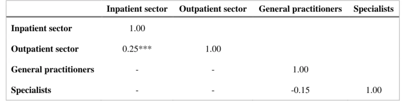
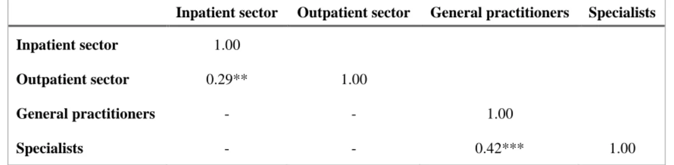
The regression analysis uses the same covariates as the one performed in part one, how- ever, it consists of four separate equations, one for each health care sector (inpatient and outpatient sector) or speciality (general practitioners and specialists) and two estima- tions: In the first estimation, a SUR model will be performed in order to find out wheth- er there is a relationship between health expenditures of different health care sectors while the second estimation applies this issue to different specialities in the outpatient sector. When interpreting the results of these estimations, the covariance matrices as measures of linear dependence between two random variables will also be closely ex- amined. To that end, a Breusch-Pagan test, which tests for independent equations, will be performed. The statistical test will be significant if the equations, and the variables, are dependent on each other, i.e. if the disturbance covariance matrix is not diagonal (Stata, 2020).
All in all, the methodological approach in part two aims at establishing a relationship between health expenditures of different health care sectors and specialities as well as at looking at the determinants of these expenditures. To that end, a correlation analysis as well as SUR models will be used.
𝑖 stands for the relevant district
𝑗 stands for the relevant health care sector/speciality 𝑦 = health care expenditures per inhabitant
𝑋 1 = vector of supply of health services
𝑋 2 = vector of demand of health services
𝜀 = stochastic error term
24 5 RESULTS
Applying the empirical strategy to the data, the following results could be achieved and are further presented in section 5.1 (regional variation of health care expenditures) and section 5.2 (relationship between health expenditures in different health care sectors and specialities).
5.1 Regional variation of health care expenditures
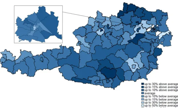
The results of the descriptive analysis of regional disparities show that in 2016, there was indeed regional variation of health care expenditures in Austria. Figure 5 displays the regional variation of total expenditures as deviation from the mean whereby lighter colours stand for below-average and darker ones for above-average health care expendi- tures.
Note: In addition to the district excluded from the analysis for data protection reasons, the district "Wien- Umgebung" is also highlighted in white, as this district was dissolved in the course of a district reform in 2017.
Data source: Main Association of Austrian Social Security Institutions
In 2016, total expenditures varied between 50% below and 30% above the Austrian av- erage of 1,844.15€ per inhabitant at the district-level (see Figure 5). Even though no clear pattern can be discerned when looking at the map, some individual districts exhib- ited particularly high or low health expenditures. The existence of regional disparities in
Figure 5: Regional variation of total (health care) expenditures per inhabitant
25
health care expenditures can also be confirmed by the coefficient of variation which was 0.10 and points therefore clearly to regional variation of health expenditures in Austria.
As a second step, the determinants of health care expenditures were estimated using a multiple linear regression model in order to explore the different district-level health care expenditures per inhabitant. The regression results are displayed in Table 3. Note that model 1 is a restricted model and includes the supply of physicians for the supply side as well as the morbidity and mortality of the population for the demand side. Mod- els 2 and 3 then expand on these covariates and also include the demographic and soci- oeconomic characteristics of the population as demand-side factors. They differ, how- ever, in their standard errors so that model 3 incorporates robust standard errors.
After each estimation, regression diagnostics
13were carried out in order to determine the validity of each model. This yielded the following results: Model 1 exhibits no common inefficiencies such as heteroscedasticity and multicollinearity, but shows that relevant covariates are missing in the model. For that reason, the full model (model 2) including more demand-side variables was estimated in a second step. This corrected for the omit- ted variables, but led to heteroscedasticity in the error terms. Model 3 therefore uses the full set of covariates as well as robust standard errors which amends for inefficiencies such as heteroscedasticity as well as for the omitted variables in model 1. Looking at the goodness-of-fit measures and model selection criteria of the individual models, the full model (models 2 and 3) fares better than the restricted one at all levels: Both the R 2 (0.47 vs. 0.14) and the adjusted R 2 (0.39 vs. 0.10) are higher in models 2 and 3 than in model 1 while the AIC and BIC are lower (1,485.4 vs. 1,520.9 or 1,529.3 vs. 1,537.4).
Altogether, the regression diagnostics point to model 3 to provide the most valid results of the estimations which is why those results will be examined in more detail in the fol- lowing.
Table 3 displays the final regression results whereby the per-inhabitant health care ex- penditures per district are related to a number of covariates. Note that for the age and gender distributions, there is one reference category to which the other categories are compared to in order to avoid multicollinearity. For the age distribution, the reference
13