Assessing the representational accuracy of data-driven models: The case of the effect of urban green infrastructure on temperature

Research Collection

Journal Article

Assessing the representational accuracy of data-driven

models: The case of the effect of urban green infrastructure on temperature

Author(s):

Zumwald, Marius; Baumberger, Christoph; Bresch, David N.; Knutti, Reto Publication Date:

2021-07

Permanent Link:

https://doi.org/10.3929/ethz-b-000479923

Originally published in:

Environmental Modelling and Software 141, http://doi.org/10.1016/j.envsoft.2021.105048

Rights / License:

Creative Commons Attribution 4.0 International

This page was generated automatically upon download from the ETH Zurich Research Collection. For more

information please consult the Terms of use.

Environmental Modelling and Software 141 (2021) 105048

Available online 31 March 2021

1364-8152/© 2021 The Authors. Published by Elsevier Ltd. This is an open access article under the CC BY license (http://creativecommons.org/licenses/by/4.0/).

Assessing the representational accuracy of data-driven models: The case of the effect of urban green infrastructure on temperature

Marius Zumwald ^{a , b , *} , Christoph Baumberger ^a , David N. Bresch ^{a , c} , Reto Knutti ^b

a

Institute for Environmental Decisions, ETH Zürich, Switzerland

b

Institute for Atmospheric and Climate Science, ETH Zürich, Switzerland

c

Swiss Federal Office of Meteorology and Climatology MeteoSwiss, Zürich, Switzerland

A R T I C L E I N F O Keywords:

Urban heat Machine learning Representational accuracy Interpretable machine learning Data-driven modelling

A B S T R A C T

Data-driven modelling with machine learning (ML) is already being used for predictions in environmental sci- ence. However, it is less clear to what extent data-driven models that successfully predict a phenomenon are representationally accurate and thus increase our understanding of the phenomenon. Besides empirical accuracy, we propose three criteria to indirectly assess the relationships learned by the ML algorithms and how they relate to a phenomenon under investigation: first, consistency of the outcomes with background knowledge; second, the adequacy of the measurements, datasets and methods used to construct a data-driven model; third, the robustness of interpretable machine learning analyses across different ML algorithms. We apply the three criteria with a case study modelling of the effect of different urban green infrastructure types on temperature and show that our approach improves the assessment of representational accuracy and reduces representational uncer- tainty, which can improve the understanding of modelled phenomena.

1. Introduction

A data-driven model is a model that detects associations in data using machine learning (ML) algorithms (Knüsel and Baumberger, 2020).

Such models have been applied successfully in environmental data-science for many prediction tasks. For example, Zumwald et al.

(2021) predicted urban temperature distributions for Zürich from citi- zen weather stations (CWS), satellite and open government data. The engineering and selection of features is aided by a good understanding of the basic mechanisms that govern the temperature distribution in urban areas (Oke, 1982; Oke et al., 2017). Nevertheless, in urban planning for heat mitigation, scientific knowledge is mostly still used to propose general practical heuristics (Skelton, 2020) such as “increase (and pre- serve) the amount of urban greenery” (Thorsson et al., 2017) or “large wooded parks within a city and large trees scattered across residential areas are needed to best mitigate the urban heat island effect” (Davis et al., 2016). Such general guidelines may be helpful, but urban planning would greatly benefit from a better understanding of how different urban green infrastructure types interact with each other and influence air or ambient temperature.

Despite sufficiently high predictive accuracy, in complex modelling tasks using many features and flexible algorithms, it often remains

unclear how to make use of data-driven modelling approaches to in- crease our understanding of the mechanisms that lead to a specific urban temperature distribution pattern, because the model is based only on associations in the data which do not per se represent causal relation- ships. While there are methods that aim at extracting causal relation- ships from data (see Pearl, 2009), applications for complex spatiotemporal learning problems are still largely lacking. Here, we investigate how one can assess the representational accuracy, given pre- dictive accuracy, in order to make use of data-driven models for improving our understanding of environmental phenomena.

Zumwald et al. (2021) use citizen weather stations and machine learning to predict the temperature at high spatial and temporal reso- lutions for the city of Zürich, Switzerland. Based on this case study we investigate how supervised machine learning can be used to increase our theoretical understanding of urban temperature distribution. Even though the basic mechanisms that govern the temperature distributions in urban areas are well understood, the precise way that different sur- faces and structures such as streets, buildings and green infrastructure influence urban temperature is very complex and not sufficiently un- derstood. For example, we do not have a very good understanding of the effect of the geometry of buildings on temperature, which depends on the time of the day, the season, and the weather conditions (Konarska,

* Corresponding author. Institute for Environmental Decisions, ETH Zürich, Switzerland.

E-mail address: marius.zumwald@usys.ethz.ch (M. Zumwald).

Contents lists available at ScienceDirect

Environmental Modelling and Software

journal homepage: http://www.elsevier.com/locate/envsoft

https://doi.org/10.1016/j.envsoft.2021.105048

Accepted 26 March 2021

Holmer, et al., 2016). Here, we focus on a better understanding of the effect of different urban green infrastructure types, such as green areas, street trees, park trees and green roofs, on urban temperature distribu- tion. Methods that aim at understanding the learned relationships of a supervised machine learning algorithm are called interpretable machine learning

(IML) (Murdoch et al., 2019). Here, we use model-intrinsic feature importance metrics and the post-hoc model agnostic accumu- lated local effects (ALE) method (Apley and Zhu, 2020).

Making use of a model with low representational accuracy is a source of uncertainty. Whether a data-driven model can be used to increase our understanding of a phenomenon depends on how accurately the model represents it. Understanding requires that the model represent the phenomenon sufficiently accurately for a specific purpose. How well a data-driven model, purely based on associations, represents a target is not easy to assess. Here we propose a structured approach that aims to assess the representational accuracy of a ML model that predicts successfully.

A representationally accurate model has learned the relationships and processes that lead to the emergence of the phenomenon of interest.

However, directly evaluating the representational accuracy of a data- driven model is not possible. Empirical accuracy provides evidence that a data-driven model is representationally accurate but is not suffi- cient to exclude the possibility that the model predicts correctly for the wrong reasons. Here, we use three additional criteria to assess the representational accuracy. First, coherence with background knowl- edge. Second, robustness, i.e. the similarity of model outputs given different models (for data-driven models see Knüsel and Baumberger, 2020). We then propose a further criterion, the adequacy of the model set-up. Concerning the first criterion, we specifically investigate to what extent the model ’ s predictions and the IML outputs are consistent with background knowledge. For the second criterion, we analyze the adequacy of the measurements, datasets and methods, i.e. the model setup, which includes selecting datasets and algorithms, feature engineering training and testing procedures. Finally, for the third criterion, the robustness of the model’s predictions and the IML outputs is investigated using two ensemble algorithms, a generalized random forest (RF) (Athey et al., 2016) and XGBoost (Chen and Guestrin, 2016). In Section 2, we intro- duce the case study and the model used in this study. In Section 3, we present the results. In Section 4, we introduce our three criteria for assessing the representational accuracy of the model and use them to discuss the results critically. We conclude in Section 5 by drawing the implications of our case study for the more general question of the po- tentials and limitations of data-driven models for understanding phenomena.

2. Case study 2.1. Feature engineering

The basic mechanisms that govern the temperature distribution in urban areas are well understood (Oke, 1982; Oke et al., 2017). Green roofs can reduce thermal energy entering the indoor environment by about half (Bevilacqua et al., 2016). They can lower the outdoor roof surface and ambient temperature (for a review see Besir and Cuce, 2018) but the magnitude and spatial scale of changes are less clear. Trees are also an important measure to reduce urban heat. The cooling effect of trees can be mainly attributed to shading. But evapotranspiration con- tributes to cooling mainly around and shortly after sunset (Konarska, Uddling, et al., 2016). Furthermore, natural ground surface materials such as grass or cobblestone reduce immediate mean radiant tempera- ture, although less than direct shading by trees or buildings (Lindberg et al., 2016; Lindberg and Grimmond, 2011).

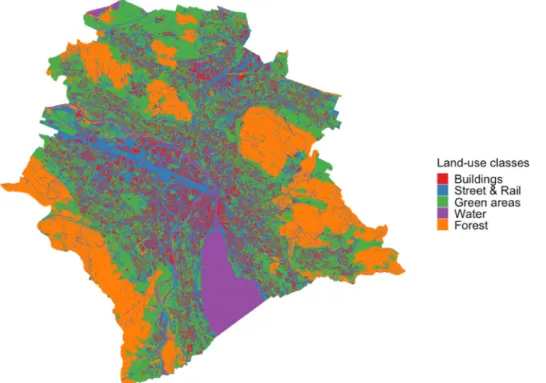
To predict urban temperature distribution, Zumwald et al. (2021) use building volume, water, forest, rail & roads, urban green areas and altitude as geographic feature groups. In this study we also use the land-use classes buildings, rail & roads, green areas, forest and water as the foundation for spatial feature engineering (see Fig. 1). The normalized differentiated vegetation index (NDVI) derived from Sentinel-2 satellite data is used as a proxy for different vegetation types.

We furthermore differentiate four urban greening categories, namely urban green areas, green roofs, park trees, and street trees. To identify green areas, we overlay the NDVI layer with the green areas geographic features and set the NDVI threshold to 0.4. Similarly, for green roofs we overlay the NDVI with a building raster and apply the same threshold.

For the trees we use a vegetation height model for Switzerland devel- oped by Ginzler and Hobi (2015), reclassify it to four classes and overlay it with a street, a rail and a green areas layer, which results in a park and street tree layer. We apply a Gaussian filter

and for the land classes count grid-cells with a certain land-use type within a 10, 30, 50, 100, 250, or 500 m radius, which leads to six features per feature group.

Altitude is an important predictor as Zürich ’ s complex topography ranges from 406 m a.s.l. to 670 m a.s.l. As we do not know the exact position above ground of the sensors, ground elevation is used as a predictor. Besides the spatial predictors, we also use 35 meteorological predictors from a MeteoSwiss weather station in Zürich. In total, 92 features were used. For a full list of the used predictors see Tables S1 and S2 in the SI.

The inclusion of further predictors might improve accuracy of the model. But the aim of this study is not to move beyond the state-of-the art in data-driven urban temperature modelling, but to test the con- ceptual framework and illustrate it with a case study.

2.2. Random forest and XGBoost

Random Forest (RF) and XGBoost (extreme gradient boosting) are both based on decision tree ensembles. The two algorithms differ in how they grow and how they combine the individual decision trees. RF relies on a procedure called bagging. Bagging stands for bootstrap aggregation and describes the process of growing individual decision trees from a random bootstrap (drawing with replacement) sample and the subse- quent aggregation of the individual trees to an ensemble. In addition to pure bagging, the RF-algorithm also draws subsamples of the features when growing a tree. This method leads to the desirable property of decorrelated features, making the application of additional cross- validation unnecessary, since bagging is already a form of internal cross-validation (except for fitting hyperparameters). The model can be evaluated repeatedly using the out-of-bag sample. Here we use the

1

IML methods are often categorized into inherently interpretable methods and model agnostic post-hoc analysis methods (Du et al., 2019). Inherent interpretability refers to methods that interpret based on the structure of the ML algorithm. Post hoc interpretability primarily refers to often model-agnostic methods that interpret the trained model without assessing the model struc- ture, relying only on the relationship between feature values and predictions.

‘Interpretation’ in the context of IML is understood as being able to explain how the algorithm derives the prediction (Doshi-Velez and Kim, 2018), with the aim of learning something about the target system (Murdoch et al., 2019). Some argue that interpretability is different for different agents and to different be- liefs and goals of different agents (Tomsett et al., 2018), hence not applying a general epistemic perspective. Others argue that what interpretability refers to is generally not clear (Lipton, 2017). Nevertheless, there are approaches to increase the use of IML methods, for example by formalizing what interpret- ability means (Dhurandhar et al., 2017) or by showing how interactive visu- alizations tools can be used in a structured workflow approach (Baniecki and Biecek, 2020).

2

We also tested a Sobel filter used for edge detection. However it did not

improve the predictive performance in the used modelling setup.

Environmental Modelling and Software 141 (2021) 105048

3

implementation from the generalized RF framework (Athey et al., 2016).

With bagging, the individual decision-trees are grown independently of each other. In contrast, XGBoost (Chen and Guestrin, 2016) is based on a procedure called boosting. Here, each tree relies on information from previous trees and the individual trees are not independent of each other. Specifically, data tuples that yielded a bad performance have an increased chance of being drawn again. The XGBoost algorithm is a computationally highly optimized and regularized stochastic gradient boosting algorithm. Allowing for regularization has the advantage of preventing overfitting, plus the stochastic gradient optimization com- putes second-order partial derivatives which often improves the per- formance of the model.

2.3. Accumulated local effects (ALE) approach

In IML, partial dependence plots (PDPs) are a model-agnostic methods to visualize the average partial relationship between the target variable and a selected feature (Friedman, 2001). However, in the case of correlated features, PDPs do not lead to reliable results, because the method assumes independent features. Furthermore, since PDPs only give an average estimate, heterogeneous effects are not visible.

Individual conditional expectation (ICE) plots aim to overcome this limitation and allow for investigation of heterogeneity across data (Goldstein et al., 2014), but still assuming independent features. Here we use the accumulated local effects (ALE) to understand the effect of individual features and their interaction on the target variable (Apley and Zhu, 2020). In contrast to PDPs and ICEs, ALE also work in the case of strongly correlated covariates since their estimation is based on the conditional distribution between features.

The algorithm sets the bin-width according to the data density. As the bins are flexible, also the rate of change is variable. ALE plots are displayed as line graphs in which each line (of each interval) represents the change in the model prediction when the selected feature has the given value compared to the average temperature prediction. The averaged prediction differences per interval are summed up along the x- axis. Hence, the ALE of a feature value that lies in the nth interval is the sum of the effects of the first through the nth interval. Finally, the

accumulated effects at each interval is centered, such that the mean effect is zero. Also, the extended approach using it in a spatial explicit way easily visualizes the effect of all features of one feature group.

Furthermore, the ALE methodology allows the investigation of the interaction of two features, which is visualized as a heat map showing the effect in addition to the individual effects.

3. Results

The RF has a root mean square error (RMSE) of 1.91

C and a mean average error (MAE) of 1.58

C on the test data, whereas the XGBoost has a RMSE of 1.37

C and MAE of 1.08

C.

In Section 3.1 the predicted temperature maps and predictions conditional on different surface types are shown. In Section 3.2 the results of the feature importance metrics are shown. In Section 3.3 the results of the IML method of ALE are presented.

3.1. Conditional predictions

Fig. 2 shows that when the model is applied to predict the temper- ature for the 30

of June 2019 at 15:00, a hot day for the district of the city of Zürich, the RF and XGBoost predict the same general patterns.

Over the city’s area, the RF has a mean of 31.5

C and XGBoost of 32.8

C. Looking only at urban green areas, RF has 31.8

C and XGBoost 32.8

C. Temperatures in areas with buildings are 32.2

C and 33.5

C respectively and thus 0.4

C and 0.7

C higher than in green areas.

Similar results hold for roads & railways, where the temperature is 32.3

C ( + 0.5

C) and 33.6

C ( + 0.8

C) respectively. Compared to green areas, park trees are marginally cooler for RF with 31.7

C and don’t change temperature for XGBoost with 32.8

C. Street trees have an average temperature of 31.5

C with the RF, which is 0.8

C lower compared to the average of railways and roads. For XGBoost the situa- tion is similar, with 32.6

C which is 1

C cooler than for the railways and roads. Fig. S1 the SI shows the temperature distribution conditional Fig. 1. Land-use classes for the city of Zürich used for feature engineering.

3

An in-depth validation of a similar modelling approach was performed by Zumwald et al. (2021).

M. Zumwald et al.

on the different surface categories.

3.2. Feature importance

In tree-based methods a frequency-based feature importance metric counts the number of times a feature is used to split across all forests.

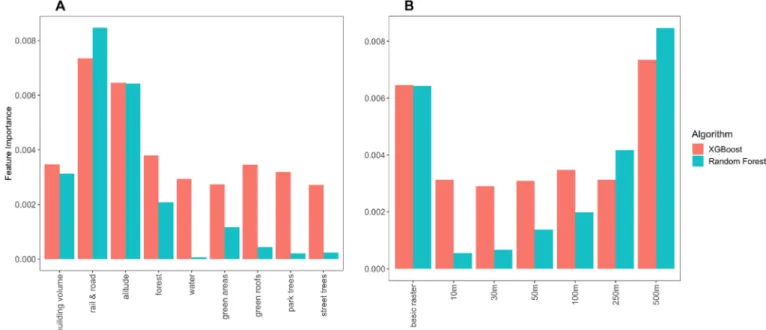
The frequency is normalized, representing the proportion that a particular feature is used to split in the trees of the model. In RF the spatial predictors sum to 4.2% whereas for XGBoost the feature impor- tance sums to 11.5%, which is nearly three times higher. Both feature importance results indicate that altitude, rail & road, and features evaluated across larger radii are more important. Fig. 3 shows how the feature importance compares across the two algorithms for altitude, building volume, street trees, park trees, green roofs and green areas summed over all features that use them. Altitude is almost equally important for both algorithms in absolute terms, but relative to the total importance of spatial variables altitude is more important for the RF algorithm. Similarly, RF assigns relatively more importance to the building volume than XGBoost. For street trees, park trees and green roofs, the RF importance is only a fraction of the XGBoost importance.

Green areas are the third most important geographic feature type for RF.

Another type of analysis aims at understanding the importance of different features of the same radius used when creating the variable.

This clearly shows for both algorithms an increase in importance with an increase in radius, with the basic raster having a resolution of 10 x 10 m.

The variable importance for the individual spatial features can be found in Fig. S3 in the SI.

The feature importance was investigated as sum of one class, and XGBoost is better in detecting signals that can be attributed to spatial factors, also explaining the better overarching performance. XGBoost also attributes greater importance to all greening-related variables than to altitude. The investigation across the spatial extent clearly shows that accounting for larger areas of influence is important to prediction.

Generally, the XGBoost assigns importance to variables at all radii, compared to RF where mostly 250 and 500 m radii are assigned greater importance. In the case of building volume, even the basic raster and 10 m raster have large importance to XGBoost.

3.3. Accumulated local effects (ALE)

To test for the strength of a monotonic non-linear relationship be- tween the ALE and the individual features we use the Kendall rank

correlation coefficient (see Abdi, 2007). Fig. 4 shows the absolute Kendall correlation coefficient for all variables with more than two levels of the respective algorithm used. Variables with a high absolute value can be considered as having a clear increasing or decreasing ordinal trend, and low absolute values are referring to a noisy signal. As a working hypothesis, we assume that any absolute value larger than 0.5 is referring to an ordinal trend and values lower than this threshold are shown gray. A negative value (blue) refers to a reduction effect on temperature, and a positive (red) to an increasing effect on temperature.

However, the Kendall rank correlation coefficient does not say anything about the magnitude of this relationship, which needs to be assessed with the feature importance (see Fig. S3 in SI). In Fig. 4, we see that for the RF the green areas feature all exhibit a trend which does not hold true for the XGBoost results. For park trees, there are 4–5 features below an absolute Kendall correlation coefficient of 0.5 in both algorithms.

Some examples of the individual ALE plots can be found in the SI (Figs. S4 and S5).

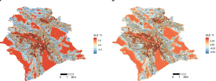
To make use of the ALE in a spatial setting, we developed spatial ALE plots. Fig. 5 shows spatial ALE plots for the green areas feature for both algorithms. Spatial ALE plots sum up ALE values for all radii per feature group per raster cell, where a feature group is defined as the combined set of features with a common geographical category and varying evaluation radii. Hence, they show the spatially explicit effect of a feature group on ALE in

C. It is clearly visible that, for instance, urban parks and greener residential areas have a cooling effect. The other spatial ALE plots can be found in Figs. S6 and S7 in the SI.

4. Understanding and reducing uncertainty due to unknown representational accuracy

The extent to which a trained ML algorithm can be used to under- stand a phenomenon depends on the representational accuracy

of the model, i.e. on how well the relationships learned by the model represent processes leading to a specific phenomenon. Moreover, using a data- driven model that has a low representational accuracy is a source of uncertainty. Assessing the representational accuracy of a model is thus Fig. 2. Temperature distribution over the city of Zürich. Map generated using Random Forest (panel A) and XGBoost (panel B). The maps show the predicted situation on the 30th June 2019 at 15:00.

4

The measurements and the features can also be inaccurate. However, we do

not discuss this in this paper. Zumwald et al. (2021) have shown that the

measurements in this study are sufficiently accurate for many purposes and that

the features rely on well-curated open satellite data and, hence, a sufficiently

high accuracy can be assumed.

Environmental Modelling and Software 141 (2021) 105048

5

of key importance. However, in contrast to its predictive accuracy, the representational accuracy of a model cannot be assessed directly since it is impossible to directly compare the relationships learned by the model with the physical processes that lead to a phenomenon. For this reason, we suggest three criteria that allow us to assess the representational accuracy, and thus reduce the representational uncertainties of data- driven models. Representational uncertainty is the lack of knowledge about how well a model represents a phenomenon. We can investigate the outputs in the results section, the conditional prediction, the feature importance and the ALE plots on two different aggregation levels, i.e. as individual features and feature groups.

It is important to note that in environmental science process-based models representing causal processes directly, e.g. via stocks and flows as in the case of climate models, do not have exactly the same challenges to interpretability as data-driven models. Process-based models can be opaque to an epistemic agent because of their computational complexity or because data that is used in model development or evaluation is itself

uncertain. Data-driven models do not presuppose any structure and learn purely from (uncertain) data. While uncertainty in data is relevant for all types of models, for data-driven models it is especially severe because erroneous data might lead an algorithm to learn incorrect structures. This has important implications concerning the interpret- ability of data-driven models. First, the uncertainty arising from datasets (e.g. measurement uncertainty) and the prediction uncertainty of the trained data-driven model are harder to separate. Second, many ML algorithms cannot optimize globally, as for example in the case of an RF (Breiman, 2001). Hence, data-driven models might miss a global opti- mum. Third, while induced randomness makes the algorithm more robust and performant, in the case of the RF it blurs the tractability compared to single-decision trees.

In section 4.1, we investigate whether the model outputs and the learned relations via IML methods are consistent with background knowledge. However, consistency with background knowledge is not sufficient to separate models that accurately represent causal relations Fig. 3. Comparison of the importance of different features summed over different categories (panel A) and radii (panel B) for the random forest and XGBoost algorithms.

Fig. 4. Kendall correlation coefficient for all 57 spatial features (altitude is only evaluated at raster- scale). The Kendall correlation coefficient indicates the strength of a rank-based, hence monotonic, relationship between the features unit and the accumulated located effect of the target variable for the RF (left) and XGBoost (right) algorithms. A negative value refers to a reduction effect on tem- perature, and a positive to an increasing effect on temperature. Absolute values lower than 0.5 are considered to show no trend are shaded gray. Only spatial features with more than 3 ALE values are considered.

M. Zumwald et al.

in the real world from those that are based on spurious correlations, as there are different levels of confidence of background knowledge and scientists want to remain open to counterintuitive findings. A reason for counterintuitive findings can be non-adequate elements in the model setup. The engineered features for example might not be adequate for the intended purpose. Hence, secondly, in section 4.2, we analyze whether the measurements, datasets and methods are adequate to construct a representationally accurate data-driven model. Thirdly, in section 4.3, robustness considerations are used to investigate whether a finding is an artefact of the ML algorithm or a spurious relationship between the data, which reduces the representational accuracy of the model. We present the analysis sequentially, but in a real case, the criteria should be applied in an iterative manner and not necessarily in any particular sequence.

4.1. Consistency with background knowledge

Background knowledge can be used to increase confidence that the trained, data-driven model correctly predicts for the right reasons, which increases our confidence that the model is representationally accurate. To assess consistency with background knowledge we first check whether the predictions, conditional on different surface types, are physically consistent, hence plausible. The models predict a tem- perature difference between green areas and roads and railways of 0.5–0.8

C in the afternoon. In the literature, similar results can be found. For instance, daytime air temperature in parks is 1 – 2

C cooler than surrounding areas, depending on the time of the day (Bowler et al., 2010; Zhang et al., 2019). Aminipouri et al. (2019) have shown that planting additional urban street trees can reduce average mean radiant temperature up to 1.3

C and hence have the potential to mitigate climate change locally under an RCP 4.5 scenario. Because our condi- tional predictions are consistent with background knowledge, this in- creases our confidence in the representational accuracy of the models.

This predictive plausibility is used to assess the emerging behavior of the model but does not per se increase our understanding of the underlying learned relationships. A model here can be consistent on the (condi- tional) predictive level but might behave as expected by chance or because of the wrong reasons. Hence consistency considerations regarding the relationships between the features need to be investigated using IML methods to rule out such behavior.

Second, we assess whether the feature importance metric results are consistent with background knowledge. Generally, based on back- ground knowledge it is difficult to form expectations about feature

importance. We know that the average environmental lapse rate is 0.65 K per 100 m altitude, hence we expect that the feature altitude is of large importance (Fig. 3). We also expect the feature group rail & roads to have a comparably large importance. The importance of different greening types is much more contested.

Third, we can check whether the ALE plots are consistent with the behavior that is expected based on background knowledge. Concerning the ALE, we use knowledge about physical processes to build hypotheses about how specific features influence temperature. For example, for the building volume, features over most radii show a positive Kendall cor- relation coefficient as one would expect, since building materials are absorbing much of incoming radiation. The basic raster and the 10-m feature do not confirm the expectation – however, there is a potential explanation for this. Building volume is also associated with shading.

The more voluminous a building, the larger a shadow it casts. In our model, we have not included this explicitly in any feature. Hence, it might be that the shade offsets the expected temperature increase close to buildings. This is a plausible explanation since temperature mea- surements probably represent conditions close to building walls, because many CWS are placed on balconies. Concerning the spatial ALE plots (Figs. S6 and S7 in the SI) the green areas, green roofs and building volume feature groups are in line with our background knowledge.

Street and park trees do not show a clear cooling effect on streets and parks.

These second and third points refer to the plausibility of the learned relations. In addition, the strength of evidence that informs any expec- tation needs to be assessed. Often background knowledge is not avail- able or is less reliable for more specific expectations, for example, at the level of explaining the behavior of individual features.

4.2. Adequacy of the model setup

One of the reasons for implausible findings can be an inadequate model setup. A signal that is detected by an IML method can be an artefact of the IML method, of the ML algorithm, or it can be based on a spurious relationship between the measurement data and some features.

It is therefore important to disentangle the adequacy of the used model setup, i.e. the measurements and features, the ML algorithm, and the IML methods and understand how they depend on each other. A better understanding of the model setup allows us to better assess represen- tational accuracy and reduce representational uncertainty.

Fig. 6 shows the relationship between the target phenomenon, the

measurement data, the features, the ML algorithm and the IML and how

Fig. 5. Spatial accumulated local effects in

C for the green areas feature group. A positive value indicates that at this location all green areas have an increasing

effect on temperature, whereas a negative value indicates a cooling effect. Panel A shows the results for the Random Forest and panel B for the XGBoost algorithm.

Environmental Modelling and Software 141 (2021) 105048

7

they depend on each other. In our case study, the crowd-sensed tem- perature measurements (1) are representing air temperature distribu- tion, which is our target phenomenon. However, a more specific understanding of the measurement conditions helps to better under- stand the adequacy of the CWS measurements. For instance, we know that there is uncertainty concerning the height of the sensor above ground (see Zumwald et al., 2021). Furthermore, many CWS measure- ments are close to building walls, hence conditions with strong back radiation from walls are overrepresented. The model features (2) are designed based on background knowledge (see Section 2.1) and our study’s key influence factors for which we want to learn a relationship with temperature. The features represent factors in the real world that influence the target phenomenon, such as urban green infrastructure, buildings and roads. We know that features affect temperature distri- bution on different spatial scales (Konarska, Holmer, et al., 2016).

Hence, we designed variations of the features taking into account different radii of influence. In total we have 92 predictors: 35 meteo- rological and 57 spatial ones. The feature engineering is limited by our available background knowledge and pragmatic considerations such as available data. An example is the rail & roads feature group with the largest feature importance. The spatial ALE of the rail & roads (see Fig. S6) indicates that this feature group seems to represent rather a general urban heat island effect rather than the expected effect of sealed surfaces such as asphalt.

An ML algorithm (3) is chosen to learn the relationship between the measurement and the features. An adequate ML algorithm needs to be sufficiently flexible. Previous studies have shown that the relationship between influence factors and urban temperature distribution do not have a high predictive accuracy when linear relationships are assumed (Voelkel and Shandas, 2017) and ensemble methods such as RF and XGBoost are more appropriate. Finally, IML approaches are used either to investigate the inner workings of the algorithm (4a) e.g. via feature importance metrics, or using model-agnostic methods in post hoc analysis (4b), in our case using ALE plots. From theory we know that ALE plots should be able to deal with correlated features (Apley and Zhu, 2020), which is important in the present case.

4.3. Robustness

If background knowledge can explain the model’s behavior, this increases confidence in the representational accuracy of the trained model. Robustness considerations can be used to further investigate the representational accuracy. Robustness indicates that a result is

insensitive to different assumptions, be it parameter values in a model, structural elements, or using different kinds of representations (Weis- berg and Reisman, 2008). Here we analyze the predictions of the different ensemble-based ML algorithms RF and XGBoost, which can be thought of as between an examination of structural and representational robustness. Generally, robustness increases the confidence that the ML algorithm is adequate to model the system under investigation, and a contradicting IML output of two different algorithms – hence a non-robust finding – means our used algorithm may not be adequate.

We investigate the robustness of the model’s mapping and condi- tional predictions, feature importance metrics and ALE plots for indi- vidual features and aggregated spatially explicit features. Fig. 2 shows the predictions for both algorithms used, and while the granularity seems different, the hotspots and patterns are robust across both algo- rithms. Furthermore, in Fig. S1 in the SI we see that the conditional predictions are also producing robust results. Concerning the feature importance, we see in Fig. 3 that the importance of different feature categories, especially those concerning green infrastructure, is not robust. The same holds true for features grouped with 10 and 30-m radii.

Generally, the XGBoost attributes more importance to the urban green infrastructure and as well as to lower radii.

For the individual features, we define robustness as the Kendall correlation between the ALE of both methods, and as a working hy- pothesis, we assume that values below 0.5 indicate a non-robust behavior and that values larger than 0.5 indicate a robust behavior (Fig. 7). For the spatial ALE plots we define robustness as the Pearson correlation between the two predicted maps and say correlations larger than 0.5 are robust. Here we choose the Pearson over the Kendall cor- relation coefficient because we aim at testing the linear relationship between the spatial ALE plots. Robustness is always interpreted together with the plausibility of a result, which is assessed using background knowledge.

In Fig. 7, the robustness is shown by the monotonic non-linear as- sociation between ALE values of the RF and the XGBoost algorithms, and non-robust relationships are shaded gray. A cross implies a both plau- sible and robust result, and we find this holds true for a minority of features. For the building volume and rail & road feature groups, a higher temperature with larger values of the features is expected (red in Fig. 4). For the remaining features a decreasing effect is expected (blue in Fig. 4). For the building volume feature group, we see that the behavior of all features can be considered robust. This might increase trust in the potential explanation of the behavior of the building volume basic raster and 10-m features, which was discussed in Section 4.1.

However, the signal could still be an artefact in the data. Although there is robustness in the general signal for green areas, the comparison in- dicates that mainly the 100-m and 50-m features are robust. The effects of green roofs and green areas are plausible and robust for smaller and mid-sized radii. Altitude and the majority of building volume features are robust and consistent with background knowledge. Rail & road only has one consistent feature, although the most important one is robust and confirms expectations. For the forest feature group, all robust fea- tures also confirm expectations as discussed in Section 4.2. When analyzing the robustness as Pearson correlation between the spatial ALE maps, the green area feature group has a Pearson correlation of 0.96, street trees of 0.57, park trees of 0.70 and green roofs of 0.74, hence all can be considered robust.

There is a trade-off between confidence in the plausibility of an effect and the adequacy of the model setup. A non-robust result containing plausible and implausible effects decreases confidence in the adequacy of the model setup more when the confidence in the plausibility assessment is high, and vice versa. For example, the modelled effect of green areas within 100 m is a robust and plausible result and increases the confidence in both the model setup and the plausibility assessment.

However, if a robust result contradicts the expected behavior, then the confidence in the expectation needs to be assessed. The higher the confidence, the more likely it is that the model setup is not adequate.

Fig. 6. Schematic overview of how (1) the measurements of the target variables and (2) the choice of features are used to represent the target phenomenon and the influence of factors such as green infrastructure. The final aim is to learn about the relationship between the influence factors and the target phenome- non by training a machine learning algorithm to learn the relationship between the measurement and the features. Model intrinsic interpretable machine learning methods (4a) such as feature importance or pots-hoc methods (4b) are used to better understand what exactly the model has learned.

M. Zumwald et al.

When the detected signal is robustly noisy, then this is likely because the model setup is not suited to detect the signal or because there is no such assumed relationship. Also, if the relationship between a feature and the target phenomenon is noisy (indicated by Kendall value close to zero in Fig. 4) and this is robust across both ML algorithms, it increases confi- dence that the finding is an artefact of the data (either the measurement or features), rather than the ML algorithm, and no real-world signal could be detected.

5. Conclusion

Increasingly high-resolution data is available (for urban areas see Creutzig et al., 2019) and the potential applications of data-driven modeling are increasing. Data-driven modeling is, for example, used to emulate spatiotemporal climate model outputs (Beusch et al., 2020), to better understand marine liquid-water clouds (Andersen et al., 2017) or to predict the dynamics of a simple general circulation model as used in numerical weather prediction models (Scher, 2018). Predictive ac- curacy is a good indicator that a model represents the target phenom- enon accurately, however it is not a sufficient condition, as the model might predict correctly for the wrong reasons (for climate models, see Baumberger et al., 2017) and overfit to noise and artefacts in the data.

To increase process understanding in earth science by deep learning methods, Reichstein et al. (2019) argue that model interpretability and physical consistency of predictions are crucial for the adoption of deep learning methods. For this purpose, knowledge about the underlying causal structure, background knowledge and appropriate methods for visualizations are also required (Zhao and Hastie, 2019).

5.1. Aiming at a better understanding of representational accuracy We have shown that the presented approach using the criteria of consistency with background knowledge, adequacy of model setup and robustness allows us to understand the representational accuracy of the

model. For example, in the presented modelling approach altitude is a single feature with no derived features and is representationally accu- rate.

The building volume features also prove to be representationally accurate. However, rail & road might, as discussed, instead represent a general urban heat island effect and cannot be considered representa- tionally accurate. Green areas and green roofs are representationally accurate on the aggregated level but not on the level of individual fea- tures. That is, we have several features (e.g. representing green roofs with different radii of influence) and fail to extract a plausible signal form the individual signals while the aggregation over all features can show some signs of representational accuracy. In contrast, park trees and street trees features are not representationally accurate individually or in aggregate. Considering green areas, a potential reason for the poor representational accuracy of individual features might be that we do not systematically investigate second-order effects between features. For example, we would expect the green area 500 m feature to exhibit a temperature reduction effect, but see the opposite (Fig. 4). To better understand the result of the implausible 500 m feature, we plotted the interaction of the 250 and 500 m features (Fig. S2 in the SI). We see that high values of the 250 m feature and values in the lower range of the 500 m feature lead to lower temperature values with an effect of up to

− 0.5

C for the XGBoost. This is an example where it is unclear whether the models overfit to an artefact in the data or whether there is an interesting relationship between green areas on different scales that needs further investigation.

Here we have investigated the robustness only on the level of different ML algorithms. However, this idea is much more generally applicable. For instance, different predictions from the same algorithms can also be used in a robustness analysis. The uncertainty of IML Fig. 7. Robustness of ALE between Random Forest and XGBoost algorithm for all 57 spatial features. Robustness is defined as the Kendall correlation coefficient larger than 0.5. The hatching represents features that confirm expectations from background knowledge in the results of the random forest. Values lower than 0.5 are considered to show no trend and are shaded gray.

5

When we refer to a feature or feature group being representationally ac-

curate, our meaning is that the relationship between this feature and the pre-

dicted temperature is representationally accurate.

Environmental Modelling and Software 141 (2021) 105048

9

outputs, if the methods allow, could also be included in the robustness analysis. Analogously to extrapolation uncertainty, IML estimates are also less reliable in data sparse regions. In a more systematic way, different elements of the model setup and not just the ML algorithm could be varied to create ensembles to more systematically investigate and reduce uncertainty. The three criteria presented here aim to indi- rectly assess the representational accuracy of a trained data-driven model and reduce representational uncertainty. While these criteria have proven to be successful for the presented case study, they can just as well be applied to other investigations in climate and environmental science.

5.2. Required representational accuracy depends on adequacy for purpose

While we cannot say that a model is representationally accurate in its entirety, it can be accurate enough for certain purposes, e.g. to answer certain questions, depending on the features and how they are repre- sented. Models that are representationally inaccurate can also be useful for other reasons. For instance, if the aim is only short term-prediction then representational accuracy is not needed. As long as we can guar- antee that the model has predicted well before and the system we predict has not changed (Knüsel et al., 2019). But as soon as we aim at under- standing the underlying phenomenon, a certain representational accu- racy becomes necessary. For example, our analysis has shown that not all individual features contribute to predictions in a way consistent with background knowledge. The green areas feature group created plausible average temperature differences between green areas and streets. In contrast we can conclude that our model cannot be used to investigate the effect of street trees, which did not show a clear temperature signal.

So besides correct conditional predictions, our model also helps to gain insights concerning certain individual features and of feature groups representing different urban greening infrastructure types.

5.3. Combining data-driven and process-based models

An approach to increase the likelihood of a representationally ac- curate data-driven model would be to constrain the data-driven model with process-based understanding in so-called hybrid models. In climate science, methods have recently been developed that can physically constrain the machine learning of evapotranspiration (Zhao et al., 2019) and achieve conservation of energy when using neural network emula- tors for global climate model emulators (Beucler et al., 2019). Using Conditional Generative Adversarial Networks it has recently been shown that urban land use can be predicted using physical constraints (Albert et al., 2019). Hence constraining data-driven models, e.g. by energy conservation approaches could in principle be applied to urban climate modelling. However applications in this domain are to the best of our knowledge still lacking. Knowledge about physical processes might also be used to further improve the feature engineering and increase the representational accuracy of models. One possible example is to explicitly use shading patterns of buildings dependent on the time of the day as additional features.

5.4. Final remarks

It is not guaranteed that plausible results emerge just because a model represents relationships between individual features and the target variable robustly and plausibly. This potential discrepancy cannot be understood by the means of IML methods alone. We proposed three criteria to guide the assessment how accurate the data-driven model represents relationships of the phenomenon of interest: coherence with background knowledge, robustness, and the adequacy of the model set- up. By evaluating the representational accuracy via those criteria, representational uncertainty is reduced and one gets a better under- standing for which purpose the data-driven model at hand might be

adequate. This improves the value of applying data-driven models in the environmental science.

Declaration of competing interest

The authors declare that they have no known competing financial interests or personal relationships that could have appeared to influence the work reported in this paper.

Acknowledgements

We acknowledge the helpful thoughts and comments by Gertrude Hirsch Hadorn and Christopher Fairless. This study was funded by the Swiss National Science Foundation, National Research Programme 75 Big Data, project number 167215.

Appendix A. Supplementary data

Supplementary data to this article can be found online at https://doi.

org/10.1016/j.envsoft.2021.105048.

References

Abdi, H., 2007. The Kendall Rank Correlation Coefficient. Encyclopedia of Measurement and Statistics. Sage, Thousand Oaks, CA, pp. 508–510.

Albert, A., Kaur, J., Strano, E., Gonzalez, M., 2019. Spatial sensitivity analysis for urban land use prediction with physics-constrained conditional generative adversarial networks. ArXiv:1907.09543 [Cs, Stat]. http://arxiv.org/abs/1907.09543.

Aminipouri, M., Rayner, D., Lindberg, F., Thorsson, S., Knudby, A.J., Zickfeld, K., Middel, A., Krayenhoff, E.S., 2019. Urban tree planting to maintain outdoor thermal comfort under climate change: the case of Vancouver’s local climate zones. Build.

Environ. 158, 226–236. https://doi.org/10.1016/j.buildenv.2019.05.022.

Andersen, H., Cermak, J., Fuchs, J., Knutti, R., Lohmann, U., 2017. Understanding the drivers of marine liquid-water cloud occurrence and properties with global observations using neural networks. Atmos. Chem. Phys. 17 (15), 9535–9546.

https://doi.org/10.5194/acp-17-9535-2017.

Apley, D.W., Zhu, J., 2020. Visualizing the effects of predictor variables in black box supervised learning models. J. Roy. Stat. Soc. B 82 (4), 1059–1086. https://doi.org/

10.1111/rssb.12377.

Athey, S., Tibshirani, J., Wager, S., 2016. Generalized random forests. ArXiv:1610.01271 [Econ, Stat]. http://arxiv.org/abs/1610.01271.

Baniecki, H., Biecek, P., 2020. The grammar of interactive explanatory model analysis.

ArXiv:2005.00497 [Cs, Stat]. http://arxiv.org/abs/2005.00497.

Baumberger, C., Knutti, R., Hirsch Hadorn, G., 2017. Building confidence in climate model projections: an analysis of inferences from fit. Wiley Interdiscipl. Rev.: Clim.

Change 8 (3). https://doi.org/10.1002/wcc.454 n/a-n/a.

Besir, A.B., Cuce, E., 2018. Green roofs and facades: a comprehensive review. Renew.

Sustain. Energy Rev. 82, 915–939. https://doi.org/10.1016/j.rser.2017.09.106.

Beucler, T., Rasp, S., Pritchard, M., Gentine, P., 2019. Achieving conservation of energy in neural network emulators for climate modeling. ArXiv:1906.06622 [Physics]. htt p://arxiv.org/abs/1906.06622.

Beusch, L., Gudmundsson, L., Seneviratne, S.I., 2020. Emulating Earth system model temperatures with MESMER: from global mean temperature trajectories to grid- point-level realizations on land. Earth Syst. Dynam. 11 (1), 139–159. https://doi.

org/10.5194/esd-11-139-2020.

Bevilacqua, P., Mazzeo, D., Bruno, R., Arcuri, N., 2016. Experimental investigation of the thermal performances of an extensive green roof in the Mediterranean area. Energy Build. 122, 63–79. https://doi.org/10.1016/j.enbuild.2016.03.062.

Bowler, D.E., Buyung-Ali, L., Knight, T.M., Pullin, A.S., 2010. Urban greening to cool towns and cities: a systematic review of the empirical evidence. Landsc. Urban Plann. 97 (3), 147–155. https://doi.org/10.1016/j.landurbplan.2010.05.006.

Breiman, L., 2001. Random forests. Mach. Learn. 45 (1), 5–32.

Chen, T., Guestrin, C., 2016. Xgboost: a scalable tree boosting system. In: Proceedings of the 22nd Acm Sigkdd International Conference on Knowledge Discovery and Data Mining, pp. 785–794.

Creutzig, F., Lohrey, S., Bai, X., Baklanov, A., Dawson, R., Dhakal, S., Lamb, W.F., McPhearson, T., Minx, J., Munoz, E., Walsh, B., 2019. Upscaling urban data science for global climate solutions. Global Sustain. 2 https://doi.org/10.1017/sus.2018.16.

Davis, A.Y., Jung, J., Pijanowski, B.C., Minor, E.S., 2016. Combined vegetation volume and

greenness

affect urban air temperature. Appl. Geogr. 71, 106

114. https://doi.

org/10.1016/j.apgeog.2016.04.010.

Dhurandhar, A., Iyengar, V., Luss, R., Shanmugam, K., 2017. A formal framework to characterize interpretability of procedures. ArXiv:1707.03886 [Cs]. http://arxiv.

org/abs/1707.03886.

Doshi-Velez, F., Kim, B., 2018. Considerations for evaluation and generalization in interpretable machine learning. In: Escalante, H.J., Escalera, S., Guyon, I., Bar

o, X., Güçlütürk, Y., Güçlü, U., van Gerven, M. (Eds.), Explainable and Interpretable Models in Computer Vision and Machine Learning. Springer International Publishing, pp. 3–17. https://doi.org/10.1007/978-3-319-98131-4_1.

M. Zumwald et al.

Du, M., Liu, N., Hu, X., 2019. Techniques for interpretable machine learning. Commun.

ACM 63 (1), 68

77. https://doi.org/10.1145/3359786.

Friedman, J.H., 2001. Greedy function approximation: a gradient boosting machine.

Ann. Stat. 29 (5), 1189–1232 (JSTOR).

Ginzler, C., Hobi, M.L., 2015. Countrywide stereo-image matching for updating digital surface models in the framework of the Swiss national forest inventory. Rem. Sens. 7 (4), 4343–4370. https://doi.org/10.3390/rs70404343.

Goldstein, A., Kapelner, A., Bleich, J., Pitkin, E., 2014. Peeking inside the black box:

visualizing statistical learning with plots of individual conditional expectation.

ArXiv:1309.6392 [Stat]. http://arxiv.org/abs/1309.6392.

Knüsel, B., Baumberger, C., 2020. Understanding climate phenomena with data-driven models. In: Studies in History and Philosophy of Science Part A. https://doi.org/

10.1016/j.shpsa.2020.08.003.

Knüsel, B., Zumwald, M., Baumberger, C., Hirsch Hadorn, G., Fischer, E.M., Bresch, D.N., Knutti, R., 2019. Applying big data beyond small problems in climate research. Nat.

Clim. Change 9 (3), 196–202. https://doi.org/10.1038/s41558-019-0404-1.

Konarska, J., Holmer, B., Lindberg, F., Thorsson, S., 2016a. Influence of vegetation and building geometry on the spatial variations of air temperature and cooling rates in a high-latitude city. Int. J. Climatol. 36 (5), 2379–2395. https://doi.org/10.1002/

joc.4502.

Konarska, J., Uddling, J., Holmer, B., Lutz, M., Lindberg, F., Pleijel, H., Thorsson, S., 2016b. Transpiration of urban trees and its cooling effect in a high latitude city. Int.

J. Biometeorol. 60 (1), 159

172. https://doi.org/10.1007/s00484-015-1014-x.

Lindberg, F., Grimmond, C.S.B., 2011. The influence of vegetation and building morphology on shadow patterns and mean radiant temperatures in urban areas:

model development and evaluation. Theor. Appl. Climatol. 105 (3), 311–323.

https://doi.org/10.1007/s00704-010-0382-8.

Lindberg, F., Onomura, S., Grimmond, C.S.B., 2016. Influence of ground surface characteristics on the mean radiant temperature in urban areas. Int. J. Biometeorol.

60 (9), 1439–1452. https://doi.org/10.1007/s00484-016-1135-x.

Lipton, Z.C., 2017. The mythos of model interpretability. ArXiv:1606.03490 [Cs, Stat].

http://arxiv.org/abs/1606.03490.

Murdoch, W.J., Singh, C., Kumbier, K., Abbasi-Asl, R., Yu, B., 2019. Interpretable machine learning: definitions, methods, and applications. Proc. Natl. Acad. Sci. Unit.

States Am. 116 (44), 22071–22080. https://doi.org/10.1073/pnas.1900654116.

Oke, T.R., 1982. The energetic basis of the urban heat island. Q. J. R. Meteorol. Soc. 108 (455), 1–24. https://doi.org/10.1002/qj.49710845502.

Oke, T.R., Mills, G., Christen, A., Voogt, J.A., 2017. Urban Climates. Cambridge University Press. https://doi.org/10.1017/9781139016476.

Pearl, J., 2009. Causality. Cambridge university press.

Reichstein, M., Camps-Valls, G., Stevens, B., Jung, M., Denzler, J., Carvalhais, N., Prabhat, 2019. Deep learning and process understanding for data-driven Earth system science. Nature 566 (7743), 195–204. https://doi.org/10.1038/s41586-019- 0912-1.

Scher, S., 2018. Toward data-driven weather and climate forecasting: approximating a simple general circulation model with deep learning. Geophys. Res. Lett. 45 (22) https://doi.org/10.1029/2018GL080704, 12,616-12,622.

Skelton, M., 2020. How cognitive links and decision-making capacity shape sectoral experts’ recognition of climate knowledge for adaptation. Climatic Change 162 (3), 1535–1553.

Thorsson, S., Rayner, D., Lindberg, F., Monteiro, A., Katzschner, L., Lau, K.K.-L., Campe, S., Katzschner, A., Konarska, J., Onomura, S., Velho, S., Holmer, B., 2017.

Present and projected future mean radiant temperature for three European cities. Int.

J. Biometeorol. 61 (9), 1531–1543. https://doi.org/10.1007/s00484-017-1332-2.

Tomsett, R., Braines, D., Harborne, D., Preece, A., Chakraborty, S., 2018. Interpretable to Whom? A Role-Based Model for Analyzing Interpretable Machine Learning Systems.

ArXiv Preprint ArXiv:1806.07552.

Voelkel, J., Shandas, V., 2017. Towards systematic prediction of urban heat islands:

grounding measurements, assessing modeling techniques. Climate 5 (2), 41. https://

doi.org/10.3390/cli5020041.

Weisberg, M., Reisman, K., 2008. The robust volterra principle. Philos. Sci. 75 (1), 106

131. https://doi.org/10.1086/588395.

Zhang, J., Gou, Z., Shutter, L., School of Engineering and Built Environment, Griffith University, Australia, 2019. Effects of internal and external planning factors on park cooling intensity: field measurement of urban parks in Gold Coast, Australia. AIMS Environ. Sci. 6 (6), 417–434. https://doi.org/10.3934/environsci.2019.6.417.

Zhao, Q., Hastie, T., 2019. Causal interpretations of black-box models. J. Bus. Econ. Stat.

https://doi.org/10.1080/07350015.2019.1624293, 1–10.

Zhao, W.L., Gentine, P., Reichstein, M., Zhang, Y., Zhou, S., Wen, Y., Lin, C., Li, X., Qiu, G.Y., 2019. Physics-Constrained machine learning of evapotranspiration.

Geophys. Res. Lett. 46 (24), 14496–14507. https://doi.org/10.1029/

2019GL085291.

Zumwald, M., Knüsel, B., Bresch, D.N., Knutti, R., 2021. Mapping urban temperature

using crowd-sensing and machine learning. Urban Climate 35, 100739.