natural nonlinear interactions between stock and foreign exchange markets

On the inherent instability of international financial markets:

natural nonlinear interactions between stock and foreign exchange markets

Roberto Dieci Frank Westerhoff

Working Paper No. 79 April 2011

k*

b

0

B A M

AMBERG CONOMIC

ESEARCH ROUP

B E R G

Working Paper Series BERG

on Government and Growth

Bamberg Economic Research Group on Government and Growth

Bamberg University Feldkirchenstraße 21

D-96045 Bamberg

Telefax: (0951) 863 5547

Telephone: (0951) 863 2547

E-mail: public-finance@uni-bamberg.de

http://www.uni-bamberg.de/vwl-fiwi/forschung/berg/

Reihenherausgeber: BERG Heinz-Dieter Wenzel Redaktion

Felix Stübben

On the inherent instability of international financial markets:

natural nonlinear interactions between stock and foreign exchange markets

Roberto Dieci

and Frank Westerhoff

a

University of Bologna, Department of Mathematics for Economic and Social Sciences

b

University of Bamberg, Department of Economics

Abstract

We develop a novel financial market model in which the stock markets of two countries are linked via and with the foreign exchange market. To be precise, there are domestic and foreign speculators in each of the two stock markets which rely either on linear technical or linear fundamental trading strategies to determine their orders. Since foreign stock market speculators require foreign currency to conduct their trades, all three markets are connected. Our setup entails a natural nonlinearity which may cause persistent endogenous price dynamics. Moreover, we analytically show that market interactions can destabilize the model’s fundamental steady state.

Keywords

Stock prices; exchange rates; market stability; technical and fundamental analysis;

nonlinear market interactions; endogenous dynamics.

JEL classification C63; F31; G12; G14.

______________

*

Contact: Frank Westerhoff, University of Bamberg, Department of Economics, Feldkirchenstraße 21,

D-96045 Bamberg, Germany. Email: frank.westerhoff@uni-bamberg.de

1 Introduction

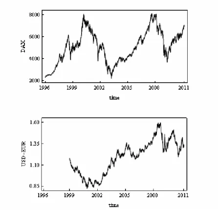
Recurrent dramatic upward and downward movements of international asset prices raise the question whether our global financial system is inherently unstable. Consider, for instance, the course of major stock markets since the mid 1990s. First we saw the emergence of the dot-com bubble and its consequent crash. Afterwards, many stock markets around the world recovered, reaching even previous highs, but only to collapse once again in the second half of 2007. How spectacular such long-term price swings can be is visible in the top panel of Figure 1, which displays the evolution of the German stock market index, the so-called DAX, between 1996 and 2010. The DAX more than tripled its value twice, and yet it lost about half of its value twice, too. A similar worrying picture emerges with respect to foreign exchange markets. The strong shifting behavior of the USD-EUR exchange rate, depicted in the bottom panel of Figure 1, is only one of many stunning examples. After a shaper downward movement between 1999 and 2002, the USD-EUR exchange rate almost doubled its value by 2008, only then to lose a substantial part of its value again. Comprehensive historical accounts of such phenomena and their macroeconomic consequences are provided by Kindelberger (1978), Minsky (1982), Galbraith (1997), Shiller (2003) and Akerlof and Shiller (2008).

--- Figure 1 about here ---

Without doubt, a crucial question is thus what kind of mechanisms may cause

such dynamics. While no monocausal explanation is to be expected here, our paper

points out that integrated international financial markets may be prone to severe price

fluctuations. To be precise, we show that stock and foreign exchange markets are – by

construction – nonlinearly interwoven and that interactions between them may give rise

to endogenous dynamics. Our results are based on a model which has the following

structure. We consider two countries, called countries H(ome) and A(broad). Both countries have a stock market in which the market participants (speculators) use either technical or fundamental analysis rules to predict the future direction of the markets.

Hence, there are four types of traders in each stock market: domestic chartists, domestic fundamentalists, foreign chartists and foreign fundamentalists. In order to highlight the nonlinear connection between the markets, we design the model as simply as possible.

In particular, the relative importance of the four trader types is constant over time and their trading strategies are linear. Moreover, the price adjustments in the stock and foreign exchange markets are proportional to the traders’ excess demands.

It is important to note that the stock markets are linked via and with the foreign exchange market. First, technical traders who trade abroad take both the stock price trend and the exchange rate trend into account. Second, fundamental traders who trade abroad condition their orders on both mispricing on the foreign stock market and mispricing on the foreign exchange market. Third, the transactions of foreign traders go through the foreign exchange market. Suppose, for instance, that a trader from country A wants to buy stocks in country H. Then this trader obviously also trades on the foreign exchange market to obtain foreign currency for the stock purchase. The amount of foreign currency required is a nonlinear function: the demand for stocks, which is a function of current and/or past stock prices, is multiplied by the current stock price. This nonlinearity, which has a quite natural foundation, is the only nonlinearity within our model. But, as we will see, its impact on the dynamics is not to be underestimated.

Simulations of our model – a six-dimensional nonlinear dynamic system – reveal

that interactions between stock and foreign exchange markets may trigger endogenous

dynamics. That is, the stock prices of the two countries and the associated exchange rate

oscillate continuously around their fundamental values for a broad range of parameter values. Moreover, we also establish the destabilizing nature of market interactions analytically in the form of a (local) stability analysis. Irrespective of whether there are interactions between the markets, our model has a unique steady state in which prices properly reflect their fundamental values. Roughly speaking, we find that if the steady state of the model with isolated stock markets is unstable, then the steady state of the model with market interactions is also unstable. However, if the steady state of the model with isolated stock markets is stable, the steady state of the model with market interactions may be unstable. In this sense, market interactions can be regarded as a destabilizing force for the dynamics of international financial markets. Our results also indicate that regulating financial markets is a complicated issue since causalities acting inside our model may run against basic economic intuition.

Our paper is part of the burgeoning field of agent-based financial market modeling (for recent surveys see Chiarella et al. 2009, Hommes and Wagener 2009, Lux 2009 and Westerhoff 2009, among others). Guided by empirical evidence

, a number of interesting approaches have been proposed in the last 20 years which help us to explain the behavior of financial markets. Let us briefly categorize the main mechanisms discussed so far.

- In Day and Huang (1990), Chiarella (1992), Chiarella et al. (2002) and Farmer and Joshi (2002), endogenous dynamics arise since the trading behavior of destabilizing technical and/or stabilizing fundamental traders is nonlinear. For instance, technical

1

Empirical evidence showing that financial market participants rely on technical and fundamental trading

rules to determine their orders is overwhelming, see Hommes et al. (2005), Menkhoff and Taylor (2007),

Menkhoff et al. (2009), Heemeijer et al. (2009), among others. These results strengthen the view that

agents are boundedly rational (Simon 1982, Kahneman et al. 1986, Smith 1991).

traders may be more aggressive than fundamental traders when prices are close to the fundamental value and their orders can thus initiate a bubble. However, fundamental traders may become more aggressive as the bubble continues to grow and trigger some kind of mean reversion.

- In other models, e.g. by Kirman (1991), Lux (1995) and Brock and Hommes (1998), speculators switch between technical and fundamental analysis (e.g. due to herding dynamics, market conditions or the rules past performance). A market may thus be unstable if speculators prefer technical trading but turns stable if they switch to fundamental analysis.

- Finally, Westerhoff (2004), Chiarella et al. (2005), Westerhoff and Dieci (2006) and Chiarella et al. (2007) consider multi-asset market dynamics. For instance, in these models a market may be stable as long as fundamental traders are in the majority.

However, if there is a temporary inflow of technical traders (who may previously have traded elsewhere) the market may temporarily become unstable.

To sum up, while most models proposed so far consider that agents use nonlinear trading rules, switch between competing trading strategies and/or markets, our paper additionally points out that stock and foreign exchange markets are – by construction – nonlinearly interwoven and that this can give rise to instability and the onset of endogenous dynamics.

The rest of our paper is organized as follows. In Section 2, we introduce a novel model in which the dynamics of two stock markets and one foreign exchange market are linked. In Sections 3 and 4 we present our analytical and numerical results, respectively.

Section 5 concludes the paper. A number of proofs are given in the Appendix.

2 The model

In this section, we develop a model with interdependent stock and foreign exchange markets. For simplicity, we concentrate on a two-country setup and label the two countries H(ome) and A(broad). Both countries have their own currency. In each of the two stock markets there are four types of traders: chartists from countries H and A and fundamentalists from countries H and A. In general, chartists bet on a continuation of price trends while fundamentalists try to exploit mispricings. We assume that all traders rely on linear trading rules and that their market impact is constant over time. No speculators focus explicitly on the foreign exchange market.

However, stock market traders from abroad require foreign currency to conduct their trade. Moreover, their stock market orders depend on the expected future course of the exchange rate and thus the two stock markets are linked via and with the foreign exchange market. The model is closed by postulating positive relations between price changes and excess demands in all three markets.

We proceed as follows. In Sections 2.1 to 2.3, we characterize the stock market in country H, the stock market in country A and the foreign exchange market, respectively. In Section 2.4, we summarize the structure of our model. As we will see, its dynamics is driven by three coupled second-order difference equations.

2.1 The stock market in country H

We start by modeling the stock market in country H. Let P

be the log stock price of

2

Dieci and Westerhoff (2010) add nonlinear foreign exchange speculation to a simplified version of our framework. They find that foreign exchange speculators who switch between technical and fundamental trading rules may generate intricate bubbles and crashes in the foreign exchange market which then spillover to stock markets, from which they feed back towards the foreign exchange market, and so on.

Such a framework is also studied in Tramontana et al. (2009).

this market at time step t . Since log stock prices adjust proportionally to excess demand, we can write

)

(

1 H A

t A F Ht H C H t

Ht H C tH

tH

P D D D D

P

= + α + + +

wn.

, (1) where is a positive price adjustment parameter and , , and

are the orders of domestic chartists, domestic fundamentalists, foreign chartists and foreign fundamentalists, respectively.

α

D

D

D

A Ht

D

3

Consequently, excess buying drives the price up and excess selling drives it do

Chartists try to identify trading signals by extrapolating past price trends into the future. Orders of chartists from country H investing in market H are given by

)

(

,

,, H

H t H t H H Ht

C

P P

D = β −

, (2)

where is a positive reaction coefficient. Note that (2) implies that domestic chartists base their orders on the most recently observed price trend. For instance, if they observe an increase in the price, they optimistically submit buying orders.

H

β

Fundamentalists seek to profit from mean reversion. Orders of fundamentalists from country H active in market H are written as

)

,

(

,, H

H t H H H Ht

F

F P

D = γ − , (3)

where ^γ

is a positive reaction parameter and F

is the log fundamental value of stock market H. Hence, if stock market H is undervalued (overvalued), domestic fundamentalists perceive a buying (selling) opportunity.

Chartists from country A investing in the stock market of country H take into

3

The amount demanded by each group of speculators is proportional to a quantity or trading signal which

may be interpreted as the expected log-return from investing in the stock market (see, e.g. Dieci and

Westerhoff 2010).

account both the most recent stock market trend in country H and the most recent exchange rate trend. Therefore,

)

(

,

,, H

t H t

t A t

H A Ht

C

S P S P

D = β + −

−

, (4)

where is a positive reaction parameter and is the log exchange rate, defined as the log price of one unit of country H’s currency in terms of country A’s currency.

Suppose that the stock price and the exchange rate increase. Then this type of trader will take a buying position. If one or both trends weaken, the order size decreases. However, even a weak downward trend in one of the markets accompanied by a strong upward trend in the other market still generates buying orders.

A

β

S

We express the orders of fundamentalists from country A investing in stock market H as follows

)

,

(

,, H S t

H t A A H

Ht

F

F P F S

D = γ − + − , (5)

where is a positive reaction coefficient and is the log fundamental exchange rate. Obviously, this type of trader takes mispricing in stock market H and mispricing in the foreign exchange market into account and seeks to profit from them both.

A

γ

F

4

2.2 The stock market in country A

Since the stock market in country A is essentially a mirror image of the stock market in country H, we obtain a similar set of equations for the stock market in country A.

Accordingly, the log stock price in country A at time step t+1 is quoted as

4

Since , where lowercase letters denote absolute prices, an

alternative interpretation for trading rule (5) would be that foreign fundamentalists condition their orders on the mispricing of stock H in terms of country A’s currency. A similar argument holds, of course, for trading rule (4).

)]

/(

) [(

)

(

)

(

1 AH

t H F At A C At A F At A C tA

tA

P D D D D

P

= + α + + + , (6)

where is a positive price adjustment parameter and , , and are the orders of its four types of market participants.

α

_D

_D

_D

_D

Orders of chartists from country A trading in stock market A total )

(

,

,, A

A t A t A A

At

C

P P

D = β −

, (7) where is a positive reaction parameter. Orders of fundamentalists from country A active in stock market A amount to

A

β

)

,

(

,, A

A t A A A At

F

F P

D = γ − , (8)

where ^γ

is a positive reaction parameter and F

indicates the log fundamental value of stock market A.

Chartists from country H speculating in stock market A seek to trade )

(

,

,, A

t A t

t H t

A H At

C

S P S P

D = β − + +

−

, (9)

where is a positive reaction parameter. Finally, fundamentalists from country H active in stock market A place orders

H

β

)

,

(

,, A S t

A t H H A

At

F

F P F S

D = γ − − + , (10)

where is a positive reaction coefficient. Note that foreign traders take in (9) and (10) the inverse exchange rate into account and that the log of the reciprocal value of the exchange rate is

H

γ

t

t

S

S Exp

Log [ 1 / [ ]] = − . Similarly, − F

is the log of the inverse fundamental exchange rate.

2.3 The foreign exchange market

Changes in the log exchange rate are also proportional to excess demand. Here, excess

demand is solely due to the orders of stock traders who speculate abroad. Recall that the log exchange rate is defined as the log price of one unit of country H’s currency in terms of country A’s currency. We thus obtain

⎟ ⎟

⎠

⎞

⎜ ⎜

⎝

⎛ + − +

+

+

= ( )

] [

] ) [

](

[

1 AH

t H F At t C tA A

Ht A F Ht H C S t

t

t

D D

S Exp

P D Exp

D P Exp S

S α , (11)

where is a positive price adjustment parameter. The mechanics behind (11) are central to our paper and deserve commenting upon.

α

Note first that all stock orders are given in real units. As a result, the currency demand of traders from country A investing in country H is the product of their (real) stock transactions times the current stock prices, i.e. . Suppose that country A traders are buying stocks in country H so that this expression is positive.

Their (positive) demand for foreign currency then increases the exchange rate. A similar argument holds for traders from country H investing abroad. However, here we have to take the reciprocal value of the exchange rate into account. Moreover, if these traders buy country A’s stocks, they sell their own currency to obtain foreign currency, which

explains the minus sign in front of the term .

) ](

[ P

D

D

Exp +

) ])(

[ / ] [

( Exp P

Exp S

D

+ D

As should furthermore be clear, the nonlinearity in (11) is quite natural and not a simple ad-hoc addition to our model. It arises from price-quantity interactions and the existence of foreign stock market traders. Yet, its consequences for the model dynamics are quite significant. As we will see, such nonlinear interactions constitute a new possible explanation for the instability of international financial markets and the onset of endogenous upward and downward movements of stock prices and exchange rates.

Of course, we rely on specific functional forms for the currency demand components in

(11), based on the view that demand functions (2)-(5) and (7)-(10) represent stock

orders in physical units. In a number of related heterogeneous agent models, different specifications have been adopted.

Such alternative specifications could easily be handled within our setup by taking the more general view that demand reaction coefficients γ _{s and} β s are not fixed but state-dependent, again obtaining a nonlinear dynamical system. It can be proven that such generalizations have no impact on the analytical stability properties of the ‘fundamental steady state’, derived in the next sections. The proof is sketched in Appendix 4.

2.4 Summary

Straightforward calculations reveal that the dynamics of our model is due to a set of three coupled second-order difference equations

) , , ,

(

1 − −

+

=

tH

G P P S S

P , (12)

) , , ,

(

1 − −

+

=

tA

G P P S S

P , (13)

) , , , , ,

(

1 − − −

+

=

t

G P P P P S S

S . (14)

While the first two equations are linear, the third is (highly) nonlinear. In the following, we investigate model (12)-(14) using a combination of analytical and numerical methods.

3 Analytical results

We now present several analytical results which indicate that interacting international financial markets are more likely to be unstable than isolated national financial markets.

5

For instance, in Chiarella et al. (2002, 2005) demand functions formally similar to (2)-(5) and (7)-(10),

derived within a one-period mean-variance setup, represent the amount of wealth to be invested in the

stock market. In this case, demand in real units would be obtained through adjustments for the price (and

exchange rate) levels.

Our analytical investigation rests on the simplifying assumption that the stock markets of countries H and A are symmetric. However, in Section 4 we numerically illustrate that qualitatively similar results can also be expected in situations in which the stock markets are asymmetric. In Section 3.1, we first discuss some general characteristics of our model. We then compare the stability properties of isolated and interacting stock markets, taking two different approaches. In Section 3.2, we hold the number of speculators constant when markets open up, i.e. we consider a mere relocation of the existing mass of speculators. In Section 3.3, we allow market integration to lead to an inflow of additional foreign speculators. Section 3.4 provides insight into stock market dynamics in a regime with fixed exchange rates, as compared to a regime with flexible exchange rates.

3.1 Some preliminary insights

By introducing three auxiliary variables, model (12)-(14) can be rewritten as )

, , ,

1

(

H t H t

tH

G P U S Z

P

= , (15)

, (16) , (17)

tH tH

P U

=

) , , ,

1

(

A t A t

tA

G P U S Z P

=

tA tA

P

U

= , (18) , (19) , (20) where

) , , , , ,

1

(

A t H t H t S t

t

G P U P U S Z

S

=

t

t

S

Z

=

S HA H H HA HH H HA H HA HA H

H HA HH H H HA HH HA HH H H

H H

F F

Z S

U P

Z S U P G

γ α γ

γ α β

α γ

β α

β β α γ

γ β β α

+ +

+

−

− +

+

−

−

− + +

=

) (

) (

) (

)]

( 1 [ ) , , , (

, (21)

S AH A A AH AA A AH A AH

AH A

A AH AA A A AH AA AH AA A A

A A

F F

Z S

U P

Z S U P G

γ α γ

γ α β

α β

γ α

β β α γ

γ β β α

− +

+ +

− +

+

−

−

− + +

=

) (

) (

) (

)]

( 1 [ ) , , , (

, (22)

, (23)

i.e. the evolution of the two stock prices and the exchange rate is driven by a six- dimensional nonlinear dynamical system.

)]

( )

( )

)[(

exp(

)]

( )

( )

)[(

exp(

) , , , , , (

S A AH AH

AH AH A AH A AH AH A

S

S H HA HA HA

HA H HA H HA HA H S

A A H H S

F F Z

S U

P S

P

F F Z

S U

P P

S

Z S U P U P G

− +

+

− +

−

−

−

−

+ +

−

− +

−

− +

=

=

γ β

β γ β

γ β α

γ β γ

β β

γ β α

Obviously, one steady state of the model is given with )

, , , , , (

: = F

F

F

F

F

F

F . (24)

We call this steady state the fundamental steady state since stock prices and the exchange rate reflect their fundamental values. As a result, there is no further trade and prices are at rest. The proof of the uniqueness of this steady state is provided in Appendix 1.

For simplicity, yet without loss of generality, we assume for the price adjustment coefficients . The Jacobian matrix of our model, evaluated at its steady state, can then be expressed as

1

=

=

=

H

α α

α

: = ) (F

J (25)

,

where and . Note that the Jacobian matrix for

generic (strictly positive) reaction coefficients can be reduced to the above matrix via suitable changes of parameters, as shown in Appendix 2.

⎟⎟

⎟⎟

⎟⎟

⎟⎟

⎠

⎞

⎜⎜

⎜⎜

⎜⎜

⎜⎜

⎝

⎛

Φ + Φ

−

− Φ

−

− Φ + Φ

− Φ Φ

−

− Φ

− +

−

−

− + +

−

− +

−

−

− + +

0 1

0 0

0 0

) (

) ( ) ( 1 )

( )

(

0 0

0 1

0 0

) ( 1

0 0

0 0

0 0

0 1

0 0

) ( 1

AH A HA H AH AH A HA HA H AH A AH

AH A HA H HA

HA H

AH AH

AH AH

AA AH AA AH AA

HA HA

HA HA

HH HA HH HA HH

β β β

γ γ β β

β γ β

γ β

β β

γ β

β γ γ β β

β γ

β β

β γ γ β β

) exp(

:

H

= F

Φ Φ

: = exp( F

− F

)

The analytical study of the (local asymptotic) stability conditions of the

fundamental steady state does not appear possible in general. However, some analytical

results can be extracted in the case of symmetric markets, that is, under the following relationships between the parameters

⎪ ⎪

⎪ ⎪

⎩

⎪⎪

⎪ ⎪

⎨

⎧

Φ

= Φ

= Φ

=

=

=

=

=

=

=

=

, :

, :

, :

, :

, :

A H

AH HA F

AA HH D

AH HA F

AA HH D

γ γ γ

γ γ

γ

β β β

β β

β

(26)

where superscripts D and F now identify the demand parameters of speculators trading in their (D)omestic market and in the (F)oreign market, respectively.

In this case, the Jacobian matrix (25) turns into : =

) (F

J (27)

and tedious computations (reported in Appendix 3) allow us to factorize the 6th degree characteristic polynomial

⎟⎟

⎟⎟

⎟⎟

⎟⎟

⎠

⎞

⎜⎜

⎜⎜

⎜⎜

⎜⎜

⎝

⎛

Φ

−

− Φ + Φ

− Φ

− Φ

−

− Φ

− +

−

−

− + +

−

− +

−

−

− + +

0 1

0 0

0 0

2 ) (

2 1 )

( )

(

0 0

0 1

0 0

) (

1 0 0

0 0

0 0

0 1

0 0

) (

1

F F

F F

F F F

F F

F F

F F

D F D F D

F F

F F

D F D F D

β γ

β β

γ β β

γ β

β β

γ β

β γ γ β β

β γ

β β

β γ γ β β

) ( λ

P of the Jacobian matrix (27) as ),

( ) ( )

( λ _P

λ _P

λ

P = (28)

where _P

( λ ) is a 4th degree polynomial and _P

( λ ) is a 2nd degree polynomial. The latter expression reads

).

( ) 1

( )

(

2 D F D F D F

P λ = λ − + β + β − γ − γ λ + β + β (29)

As we will see, this factorization enables us to perform, in the reference case of

symmetric markets, a rather exhaustive comparison of the stability conditions for the

system of interacting markets with the stability conditions we obtain when stock

markets are independent.

Let us therefore consider next the case in which speculators are not allowed to trade abroad (i.e. ). The dynamics of the two stock markets of countries H and A are then given by two uncoupled two-dimensional linear dynamical systems. To be precise, the stock prices in the two countries evolve according to

0

=

=

F

γ β

i D ti D ti D D

ti

P U F

P

= ( 1 + β − γ ) − β + γ , (30)

ti ti

P

U

= , (31)

with i ∈ { H , A } , having unique fundamental fixed points P

= U

= F

. The characteristic polynomial associated with (either of) the two isolated symmetric stock markets is given by

D D

Q ( λ ) = λ

− ( 1 + β

− γ ) λ + β , (32) and necessary and sufficient conditions for the (global asymptotic) stability of the fundamental steady state can be written as

⎪⎩

⎪ ⎨

⎧

<

+

<

1

) 1 ( 2

D

D D

β

β

γ . (33)

Assume now that speculators are free to choose whether to trade on their own stock market or on the foreign stock market. We distinguish between the case where interactions arise via a simple relocation of the existing mass of investors (who are already active in their domestic markets) and the case where there is an inflow of additional foreign speculators. To simplify matters and to avoid additional notation, we assume that parameters , , and are proportional to the number of speculators in each group.

β

β

γ

γ

3.2 Relocation of speculators

We now compare the case of interacting markets (with characteristic polynomial (28)-

(29)) with the case of isolated markets (with characteristic polynomial (32)) by assuming that the sum of and and the sum of and are constant, i.e. we

set and , where

β

β

γ

γ

F

D

β β

β = − γ

= γ − γ

β and ^γ are fixed quantities, proportional to the total number of chartists and fundamentalists, respectively, from either country. Of course, the case of isolated markets corresponds to and . In the case of a mere relocation of speculators, therefore polynomial

β β β

= 0 ⇒

= γ

γ γ

= 0 ⇒

=

)

2

( λ

P becomes independent of β

, γ

and identical to polynomial Q ₍ λ ₎ , i.e.

β λ γ β λ

λ

λ ) = ( ) = − ( 1 + − ) +

(

2

Q

P , (34) so that in equation (28) only factor P

( λ ) is affected by the relocation (via parameters

and ). It follows that if all of the six characteristic roots of

β

γ

_P ( λ ) = _P

( λ ) _P

( λ )

have modulus smaller than one (i.e. the fundamental steady state of the system of interacting markets is locally asymptotically stable), then, a fortiori, the roots of _Q ( λ ) are also smaller than one in modulus, and therefore the isolated stock markets are stable.

Put differently, isolated unstable markets cannot be stabilized through market integration and a relocation of speculators, because stability of the integrated system requires the stability of the isolated markets.

The converse implication is not true: if _Q ( λ ) has “stable” roots, i.e. parameters β and ^γ satisfy the conditions

⎩ ⎨

⎧

<

+

<

1 ) 1 ( 2 β

β

γ , (35)

the integrated system may become unstable whenever parameters and are such that

β

γ

)

4

( λ

P has at least one “unstable” root (i.e. of modulus larger than unity). An

example of this is provided in Section 4 (see discussion of Figure 3).

To sum up, we have thus proven the destabilizing impact of market integration, whenever this is obtained through a mere relocation of existing speculators.

3.3 Market entry of additional foreign speculators

Consider now the case in which parameters and , respectively and , are not constrained to each other, which means that integration occurs via the entry of additional foreign speculators. The analysis of this case is slightly more complicated than the case of a mere relocation of speculators, yet the destabilizing effect of market interactions can again be proven, at least for a broad region of the parameter space. We obtain our results by discussing the analytical conditions (on parameters , , and ), under which polynomial

β

β

γ

γ

β

β

γ

γ

P

( λ ) in equation (28) has unstable roots, in connection with the stability conditions (on parameters and ) derived from polynomial

β

γ

) ( λ

Q in equation (32). In particular, this allows us to identify a ‘minimal’

region within the parameter space in which otherwise stable, isolated markets are destabilized by speculators who trade abroad.

First of all, it follows from (29) that the conditions

⎪⎩

⎪ ⎨

⎧

−

<

− +

+

<

F D

F F D D

β β

γ β β

γ 1

2 2

2 (36)

are necessary and sufficient for both roots of P

( λ ) to be smaller than one in modulus.

A sufficient condition for the steady state of the integrated system to be unstable is therefore that some root of _P

( λ ) is larger than one in modulus, i.e. at least one of the following inequalities holds

F F D

D

β β γ

γ > 2 + 2 + 2 − (37)

or

F

D

β

β >1 − .

(38)

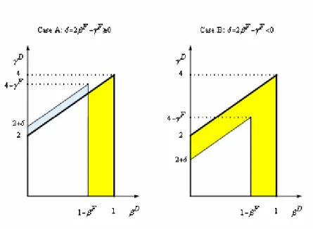
By considering these inequalities jointly with the stability conditions (33), it can be concluded that markets that are stable in case of isolation may generate an unstable integrated system in two different ways, both of which we illustrate in Figure 2. Here the area of the parameter space ( ) bounded by the axes and the thick lines represents the stability region S for the case of isolated markets. Now, depending on parameters and , a region , indicated in yellow, can be identified for which the isolated stock markets are stable but the integrated system is not.

D D

γ β ,

β

γ

R ⊂ S

--- Figure 2 about here ---

The two possible destabilization mechanisms are as follows. First, once markets become connected (due to additional speculators trading abroad), a loss of stability occurs if

) 1 (

1 − β

< β

< , (39) i.e. if foreign chartists are strong enough (indicated in both panels of Figure 2).

Second, even if , it may still be the case that parameter is so large that we have

) 1 ( 1 − <

<

D

β

β γ

) 2 2 ( 2

2

2 + β

+ β

− γ

< γ

< + β

.

(40)

Then the system is destabilized due to strong reactions of foreign fundamentalists, as depicted in the right-hand panel of Figure 2. Note that this mechanism cannot occur in a situation in which 2 β

− γ

≥ 0 , as is the case in the left-hand panel of Figure 2.

Two points deserve greater discussion. The first point concerns the region of

instability (in parameter space) for the system of integrated markets. Consider the white

region included in region S of stability of the isolated markets. In Case A (i.e.

, left-hand panel of Figure 2) this region is defined as R

S \ 0 2 β

− γ

≥

⎪⎩

⎪ ⎨

⎧

−

<

+

<

F D

D D

β β

β γ

1 2

2 ,

(41)

whereas in Case B (i.e. ^{2 β}

^{− γ}

^{< 0} , right-hand panel of Figure 2) it is specified as

⎪⎩

⎪ ⎨

⎧

−

<

− +

+

<

F D

F F D D

β β

γ β β

γ 1

2 2

2 .

(42)

We remark that in this parameter region, complementary to region R, the integrated system is not necessarily stable. In other words, the yellow area R represents only a minimal region of instability for the integrated system, because it is determined without taking into account the possible additional parameter combinations for which the roots of P

( λ ) are larger than one in modulus.

The second issue concerns the possibility that integration may stabilize otherwise unstable stock markets. This possibility depends on the starting situation.

- If but , then the isolated markets are unstable due to the behavior of trend extrapolators, and can by no means be stabilized by integration. The reason is that implies , i.e. the integrated system is unstable, too, as is also clear from Figure 2.

D

D

β

γ < 2 + 2 β

> 1

1

D

>

β β

> 1 − β

- If but , then isolated stock markets are unstable due to the overreaction of domestic fundamentalists. However, condition (36) indicates that if the foreign chartist parameter is sufficiently large (but such that ), and the foreign fundamentalist parameter is not too large, then the two roots of

1

D

<

β γ

> 2 + 2 β

β

β

< 1 − β

γ

P

( λ ) may

become smaller than unity in modulus (see the blue area in the left-hand panel of Figure

2). In this case, and if the roots of P

( λ ) are also smaller than one in modulus, unstable isolated markets become stabilized through market interactions. We present a numerical example for such an outcome in Section 4.2.

It is clear from the above discussion that market integration also tends to be destabilizing in the case of an entry of additional foreign speculators. In fact, the possibility that interactions stabilize otherwise unstable isolated markets is restricted to the particular (and rather unrealistic) case in which stock markets are unstable due to strong reactions by (domestic) fundamentalists.

Our analytical results can be summarized and interpreted as follows. There are two main mechanisms that cause the integrated system to display ‘more instability’ than the isolated stock markets. The first direct mechanism is associated with the existence of a larger amount of trading in each stock market, due to the inflow of traders from the other country. This mechanism, related to (the coefficients and the roots of) polynomial

)

2

( λ

P , determines the ‘minimal’ instability region in Figure 2, that is to say, it provides a first broad set of conditions under which interactions destabilize otherwise stable stock markets. Essentially, if the system is displaced from its steady state path due to exogenous shocks affecting only stock price H (say at time 0 and time 1), then the immediate evolution of price H (at time 2) is directly obtained by a second-order linear difference equation whose characteristic polynomial is _P

( λ ) . Comparing with the case of isolated markets (with characteristic polynomial _Q ( λ ) ), it is clear that the only difference comes from the increased strength of technical and fundamental trading ( and vs. and , respectively), by which the original parameter combination ( ) may now find itself within the yellow instability area in Figure 2.

Of course, this first mechanism is ‘inactive’ in the case of simple relocation of

F

D

β

β + γ

+ γ

β

γ

D D

γ

β _,

speculators, as proven in Section 3.2.

The second indirect mechanism operates through the exchange rate adjustments generated by the change in demand for stock. Assume, for instance, that the above described exogenous shocks to price H generate, ceteris paribus, a positive excess demand for stock H (starting from the situation of zero excess demand at the steady state). The excess demand for stock H, besides increasing price H, brings about also an upward adjustment of the exchange rate. As a consequence, next period demand for stock H, and also for stock A, from foreign traders will be affected by observed (and predicted) exchange rate movements, too, producing, in general, larger stock price adjustments than in the case of independent markets. In our model, such indirect mechanism is governed by the fourth-degree polynomial P

( λ ) . Its impact on the dynamics may be quite complicated, and sometimes counterintuitive, as suggested by the numerical experiments reported in Section 4.

3.4 Flexible versus fixed exchange rates

The analytical results presented above have largely been possible by the factorization of

the characteristic polynomial _P ( λ ) of the full model with integrated (symmetric)

markets, and by the study of the roots of factor P

( λ ) . A further straightforward

economic interpretation of the second-degree polynomial P

( λ ) is yielded from the

following thought experiment, concerning the comparison of a free floating exchange

rate regime with a system of fixed exchange rates. Intuitively, if equation (11) of the

model is replaced by a fixed (log) exchange rate S

= S = F

, ∀ t , equal to its

fundamental value, the trading behavior of foreign chartists and foreign fundamentalists

becomes equal to the trading behavior of domestic chartists and domestic

fundamentalists (there is neither a trend nor a mispricing in exchange rates and thus these trading signals vanish). As a result, the markets essentially decouple and evolve as two independent two-dimensional linear dynamical systems. In the case of symmetric markets, and using the notation introduced above, the characteristic polynomial associated with each of the two independent systems would become exactly equal to

)

2

( λ

P . The analysis carried out in this section can then also be interpreted in the sense that a change to a free floating exchange rate regime may destabilize otherwise stable stock markets.

4 Numerical results

Now we numerically illustrate some of our analytical findings. We also extend our analysis in the sense that we show that nonlinear interactions between stock and foreign exchange markets may give rise to endogenous dynamics for a broad range of parameter combinations. In Sections 4.1 and 4.2, we explore the cases where there is a simple relocation of speculators and where there is an inflow of additional foreign speculators, respectively. In Section 4.3, we turn our attention to asymmetric markets.

4.1 Relocation of speculators

In Section 3.2, we have shown that if there is a mere relocation of speculators, unstable

isolated stock markets cannot be stabilized through market interactions, yet stable

isolated stock markets may become destabilized through market interactions. To

introduce an example for the latter finding, let us first assume the parameter setting

⎪ ⎪

⎪

⎩

⎪⎪

⎪

⎨

⎧

=

=

=

=

=

=

=

=

=

=

=

=

, 00 . 0

, 65 . 0

, 00 . 0

, 60 . 0

, ,

, ,

, ,

, ,

H A A H F

A A H H D

H A A H F

A A H H D

γ γ

γ

γ γ

γ

β β

β

β β

β

(43)

i.e. speculators do not trade abroad. As can easily be verified, the steady states of both isolated stock markets are then stable, implying that after an exogenous shock, stock prices return to their fundamental values.

However, consider now that both stock markets open up and that speculators relocate on the markets as follows

⎪ ⎪

⎪

⎩

⎪⎪

⎪

⎨

⎧

=

=

=

=

=

=

=

=

=

=

=

=

. 50 . 0

, 15 . 0

, 30 . 0

, 30 . 0

, ,

, ,

, ,

, ,

H A A H F

A A H H D

H A A H F

A A H H D

γ γ

γ

γ γ

γ

β β

β

β β

β

(44)

Note that (44) implies that , ,

and . Hence, we can interpret (44) in the sense that some speculators who were previously restricted to their home markets now speculate – with the same aggressiveness – abroad.

6 . 0

,

,^H

+

=

H

β

β β

+ β

= _{0 . 6} γ

+ γ

= _{0 . 65} 65

.

,

0

,^A

+

=

A

γ

γ

6

Moreover, let us fix (for all simulations) F

= F

= F

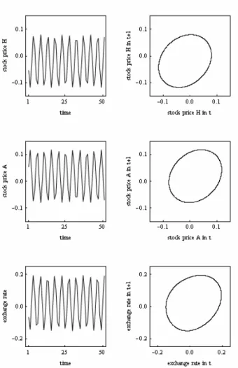
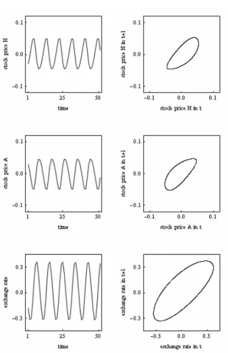
= 0 . Figure 3 shows a snapshot of the resulting dynamics. The panels show from top to bottom what is happening in stock market H, stock market A and the foreign exchange market, respectively. The left-hand panels depict the dynamics in the time domain (after a longer transient period) while the right-hand panels show the dynamics

6

Recently, several papers successfully estimated small-scale agent-based financial market models (Gilli

and Winkler 2003, Alfarano et al. 2005, Boswijk et al. 2007, Manzan and Westerhoff 2007, Franke and

Westerhoff 2010). While studies based on daily data find positive yet small values for the reaction

parameters of chartists and fundamentalists, estimates based on monthly or annual data report much larger

values. These estimates are not directly comparable to our setup but nevertheless indicate that our values

for the reaction parameters are not unreasonable, at least for a monthly, quarterly or annual perspective.

in phase space. As we can see, all three markets are characterized by quasi-periodic motion. Apparently, nonlinear market interactions, as specified in our model, can generate enduring oscillations of international asset prices.

--- Figure 3 about here ---

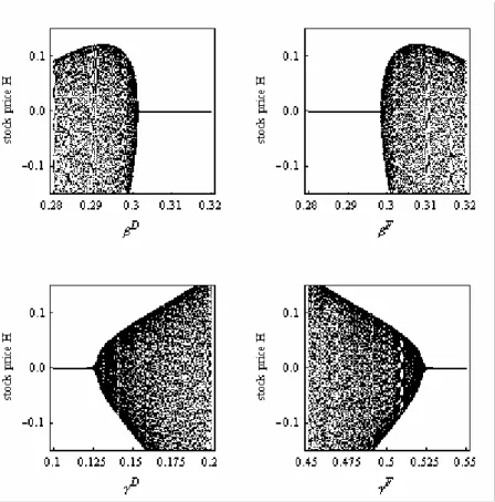
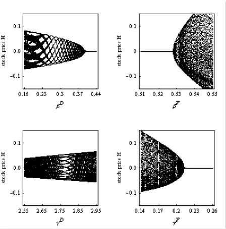
This is an important insight, and it is interesting to explore for which parameter combinations the model produces endogenous fluctuations. For this reason, we present four bifurcation diagrams in Figure 4. In each diagram we use parameter setting (44) but vary the reaction parameter indicated on the axis. Of course, in this case we assume a relocation of a fixed number of speculators and, therefore, when, e.g. parameter is increased, parameter is automatically decreased. The dynamics are plotted for the log stock price in country H.

β

D

β β

β = −

What are the results? The top right panel reveals that an increase in the aggressiveness of foreign chartists is destabilizing. If this parameter is low, we observe that stock price H converges towards its fixed point (the same is true for the other two markets). However, if this parameter exceeds a critical value, endogenous dynamics kick in. Surprisingly, a similar picture is obtained for the reaction parameter of home fundamentalists (bottom left). If this trader type is too aggressive, a system of interdependent markets becomes unstable. Symmetrically, the top left panel shows that more aggressive domestic chartists tend to stabilize the markets. Finally, also more aggressive foreign fundamentalists are apparently conducive to market efficiency (bottom right). To summarize, when agents relocate across the two stock markets, an

7

Should policy makers now introduce a fixed exchange rate regime such that the exchange rate is equal to

its fundamental value, the trading behavior of foreign fundamentalists and foreign chartists becomes

identical to the trading behavior of domestic fundamentalists and domestic chartists, respectively. As a

result, the dynamics becomes stable and stock prices converge towards their fundamental values.

increase in the impact of foreign chartists (and a simultaneous symmetric decrease in the impact of domestic chartists) is destabilizing, whereas the opposite effect is observed under an increase in the impact of foreign fundamentalists (and a simultaneous decrease in the impact of domestic fundamentalists).

--- Figure 4 about here ---

All in all, it may thus be concluded that the emergence of endogenous dynamics in a system of interrelated financial markets is quite robust, at least in the vicinity of our leading parameter setting. Moreover, the dynamic properties of our model sometimes go against standard intuition. Here we see, for instance, that more aggressive home fundamentalists destabilize the markets.

Regulatory policies which aim at stabilizing financial markets by promoting fundamental analysis in domestic markets may thus backfire. Regulatory policies have to be carefully designed in a system of interacting international financial markets.

4.2 Market entry of additional foreign speculators

It is clear from section 3.3 that the market entry of additional foreign speculators tends to be destabilizing, and numerical examples of such a scenario can easily be found. For instance, instability results if and parameters and are selected from the yellow region in the right-hand panel of Figure 2.

2

F

β

γ > β

γ

However, let us now turn to the possibility that unstable isolated stock markets may become stabilized through speculative activity from abroad. Assume the parameter setting

8

The destabilization effects observed in this example are solely due to the subset of eigenvalues related to

polynomial factor _P

( λ ) in equation (28), being polynomial _P

( λ ) unaffected by the relocation (see

equation 34).