Einf¨ uhrung in die Statistik-Umgebung R
Erste Kapitel, im Aufbau. Deutsch mit einigen englischen Abschnitten
Werner Stahel, Seminar f¨ ur Statistik ETH Z¨ urich
September 2009
c
Reproduktion f¨ur kommerzielle Zwecke
nur mit schriftlicher Bewilligung des Seminars f¨ur Statistik
Diese Unterlagen f¨uhren in die Statistik-Sprache S ein, die dem kommerziellen Pro- gramm S-Plus und der freien Software R zugrunde liegt. Da sich die Einf¨uhrung nur auf die grundlegenden Strukturen bezieht, gilt das meiste hier Geschriebene f¨ur beide Implementationen.
F¨ur den Zertifikatskurs in angewandter Statistik existieren weiterf¨uhrende Unterla- gen, die f¨ur die Themen der Bl¨ocke jeweils die n¨utzlichen Funktionen beschreiben.
2
Inhalt
1 Introduction 1
1.1 What is R? . . . 1
1.2 Other Statistical Software . . . 1
1.3 Ziele . . . 2
1.4 Einf¨uhrende Beispiele . . . 2
1.5 Using R . . . 3
1.6 Scripts and Editors . . . 5
2 Grundlagen 7 2.1 Vektoren . . . 7
2.2 Arithmetik . . . 8
2.3 Vektoren von Text . . . 9
2.4 Logische Vektoren . . . 9
2.5 Elemente ausw¨ahlen . . . 10
2.6 Matrizen . . . 11
3 Einfache Statistik 14 3.1 Einfache Statistik-Funktionen . . . 14
3.2 Tests . . . 15
3.3 Modell-Formeln . . . 16
4 Graphics 17 4.1 Overview . . . 17
4.2 Scatterplot . . . 17
4.3 Boxplot . . . 19
4.4 Adding Points and Lines to a Plot . . . 19
4.5 Adding Text to a Plot . . . 20
4.6 Interacting with a Plot . . . 21
1 Introduction
1.1 What is R?
• R is a software environment for statistical data analysis.
• R is based on commands to be typed. It implements a programming language, called theS language, which was developped for efficient statistical data analysis and for implementing statistical methods with limited effort.
• There is an inofficial menu based interfacecalled R-Commander, which contains a collection of basic statistical methods. It may be expanded by more advanced users to include methods used in their environment. This interface generates commands and submits them to the system. We will not use it here since our goal is to enable the reader to do more flexible analyses.
• Menus have the drawback that it is difficult to store or remember which buttons have to be pushed to get a certain result. Commands can be stored and thereby be used to document the analysis and allow for easy repetition with changed data, options, or other variations.
• R is free software, available from http://www.r-project.org and maintained for the operating systems Linux, Mac OS X, Windows. Therefore, every one man consulting service ...
• ... and every student and researcher who has no guts to write applications for money to purchase and maintain the system. It has therefore become the language for exchanging new methods among researchers. It gives everybody access to the newly developed tools.
1.2 Other Statistical Software
• S-Plus:This system is also based on the S language. There are differences, however, such that one could say that S-Plus and R are two dialects of this language. S-Plus is commercial, which makes it more attractive for companies who want to buy support.
It features a menu system, which is another advantage if it should be a standard software for a wide range of users.
• SPSS:This system is well known and highly developed. It contains a large collection of standard procedures, and several more advanced ones in the direction of social sciences.
• SAS: This is the classical, large statistical package – also the most expensive ge- neral package. It has developped into management of data bases and other general computer tasks. It handles large data sets, and is sometimes best for complicated analyses.
R-Kurs, cSeminar f¨ur Statistik
2 1 INTRODUCTION
• Systat:Analysis of Variance, easy-to-use graphics system.
• There are many more packages, e.g. several that are common in econometrics.
• Excel also contains statistical methods, but they are quite limited. We do not re- commend to start statistical analyses in Excel. It can profitably be used to get the dataset ready.
• Matlab is a system for mathematical calculations. The statistical methods are li- mited in both content and implementation quality. The “paradigm” is very similar to the S language, as it implements a kind of language that has similar structure as the S language but is less flexible and misses useful concepts.
1.3 Ziele
a !!!
b Some introductions into R or the S language go through the different concepts in a syste- matic way according to the structure of the language. These notes aim at starting from those notions that are needed in practice first to achieve useful results immediately. The- refore, we first introduce how a dataset is represented in R – even though this is in fact a rather complicated structure – but postpone an exact description of the concept until later.
Thus, common ways to use the system can be practiced from the start, and complications are discussed only when needed. If you prefer a more mathematical, systematic treatment, you should find other introductory texts on the web. Those documentations will also be useful as systematic references once you have worked through this script.
c The participants and readers should be able to conduct statistical analyses as they will know how to handle R and how to get the necessary information for finding and using specific methods. They should have the basic knowledge for exploiting the flexibility of the system by programming and writing their own functions.
1.4 Einf¨ uhrende Beispiele
a Daten, data.frame. Statistische Auswertungen gehen in den meisten F¨allen von einer
”Datentabelle“ oderDatenmatrixaus. In einer Zeile dieser Tabelle stehen die Werte aller Variablen(oder Merkmale), die zu einer Beobachtung geh¨oren. In S sind sie in einem so genanntendata.framegespeichert. Die Variablen k¨onnen numerisch (quantitativ) oder nominal (kategorial) sein (oder sogar komplexe Zahlen).
b Daten einlesen. Um den ersten Datensatz f¨ur das System verf¨ugbar zu machen, rufen wir die S-Funktion read.tableauf. Der Befehl
> d.sport <− read.table(
"http://stat.ethz.ch/Teaching/Datasets/WBL/sport.dat",header=TRUE) liest die Daten der Textdatei ”sport.dat” von der angegebenen Internetseite und speichert sie unter dem Namend.sportab.
Mit diesem Befehl greifen Sie ¨uber das Internet direkt auf den vom Seminar f¨ur Stati-
1.5. USING R 3
c Datensatz d.sport Nun tippen wir
> d.sport
in die R-Console. Dann erscheint auf dem Bildschirm
weit kugel hoch disc stab speer punkte OBRIEN 7.57 15.66 207 48.78 500 66.90 8824 BUSEMANN 8.07 13.60 204 45.04 480 66.86 8706 DVORAK 7.60 15.82 198 46.28 470 70.16 8664
: : : : : : : :
: : : : : : : :
: : : : : : : :
CHMARA 7.75 14.51 210 42.60 490 54.84 8249 d Eine Variable ausw¨ahlen
> d.sport[,"kugel"]
w¨ahlt die Variable ”kugel” aus. (Die eckigen Klammern w¨ahlen Teile von data.frames und anderen
”Objekten “ aus.
e Ein Histogramm. Die Funktionhistzeichnet ein Histogramm in ein Grafik-Fenster:
> hist(d.sport[,"kugel"])
Im R wird ein solches Fenster automatisch ge¨offnet, wenn noch keines
”aktiv“ ist. (In ¨alte- ren S-Plus-Versionen m¨usste man eine Funktion aufrufen, z.B.wingraph()odermotif().) f Streudiagramme. Eine der grundlegendsten grafischen Darstellungen ist sicher das
Streudiagramm.
> plot(d.sport[,"kugel"], d.sport[,"speer"])
tr¨agt die Werte der Variablen kugelinx-Richtung und speeriny-Richtung auf.
g Streudiagramm-Matrix.
> pairs(d.sport)
erzeugt eine ganze Matrix von Streudiagrammen nach dem Prinzip
”jede Variable der Datenmatrix d.sportgegen jede “.
1.5 Using R
a Let us resume basic characteristics of using R.
• Within a window running R, you will see the prompt >. You type a command and get a result and a new prompt.
stik f¨ur den Weiterbildungslehrgang zur Verf¨ugung gestellten Datensatz
”sport.dat“ zu. Sie k¨onn- ten den Datensatz auch zuerst auf Ihrer Hard-Disc speichern – indem Sie ihn auf der Websei- te anklicken und dann mittels Datei/Speichern an einem geeigneten Ort, z. B. in einem Ordner C:/EigeneDateien/Datasets ablegen. Der Befehl zum Einlesen des Datensatzes lautet dann: d.sport
<− read.table("C:/EigeneDateien/Datasets/sport.dat", header=TRUE).
4 1 INTRODUCTION
An incomplete statement can be continued on the next line
> plot(d.sport[,"kugel"], + d.sport[,"speer"])
• R stores“objects”in your“workspace”:
> d.sport <- read.table(...)
defines the objectd.sport. More specifically, d.sport is a “data.frame”.
• Objects have names like a, fun, d.sport . Names start by a letter and are continued by letters or digits. The dot (.) and underscore ( ) are treated like letters.
Blanks and special characters terminate the name. Upper and lower case letters are distinct.
There are, of course, some reserved names, likeif,for,break. The system will issue an error message if you try to use one of them to store your own stuff. Then, there are some hazards: You can overwrite basic functions or constants (as by pi <- 5).
• R provides a huge number of functions and other objects. This is the treasure!
There are many functions which are part of the “core system”, and even more which are provided by advanced users in so-called “packages” – and remain under their responsibility. We will come back to this point later.
b An R statement consists of
• a name of an object only. This makes the system display the object.
• a call to a function or an arithmetic expression. This leads to a graphical or numerical result (or sometimes to a “side effect” like changing an option).
• an assignment, consisting of a name, the arrow <-, and a call to a function or arithmetic expression
> a <- 2*pi/360
> mn <- mean(d.sport[,"kugel"])
stores the mean of d.sport[,"kugel"]under the namemn.
Note.The assignment can be denoted by =, but we do not recommend this since it may lead to confusion.
c Funktions-Aufruf. Funktions-Aufrufe sind das zentrale Gesch¨aft der Datenanalyse mit S.
Funktionen haben obligatorische Argumente, die das Programm braucht, um etwas Sinnvolles zu tun, beispielsweise die Daten, die ben¨utzt werden sollen. Zus¨atzlich gibt es meistens freiwillige Argumente. Werden diese weggelassen, so rechnet das Programm mit festgelegten, sinnvollen
”Weglasswerten“, so genannten Defaults. Durch die Angabe von freiwilligen Argumenten k¨onnen die festgelegten Defaults variiert werden. Beispielsweise kennthistein freiwilliges Argumentnclass.
> hist(d.sport[,"kugel"], nclass=10) produziert ein Histogramm mit ungef¨ahr 10 Klassen.
1.6. SCRIPTS AND EDITORS 5
d Help. Wir wollen die Argumente der Funktionen nicht auswendig lernen. Wenn man
> help(hist) oder
> ?hist
eintippt, erscheint in einem Fenster eine Beschreibung der Funktion hist und all ihrer Argumente – allerdings mit viel Jargon, den Sie noch nicht verstehen m¨ussen.
Oft hilft es, sich das Beispiel anzusehen, das auf der Help-Seite angef¨uhrt wird. Man kann das in R automatisch ausf¨uhren mit
> example(hist)
e Objekte. Mit der Zeit werden sich in Ihrem “workspace” immer mehr Objekte ansam- meln, die Sie gespeichert haben. Eine Liste ihrer Namen erhalten Sie mit
> objects()
Wenn Sie eines oder einige l¨oschen m¨ochten (a1und data), schreiben Sie
> rm(a1, data)
Man kann auch viele aufs Mal l¨oschen, siehe sp¨ater.
f Session beenden. Tippen Sie
> q()
bevor Sie den Computer abschalten. Das System fragt: Save workspace image? Wenn Sie y antworten, werden Ihnen in der n¨achsten Session alle
”Objekte“, die Sie in dieser Session erzeugt haben, wieder zur Verf¨ugung stehen – und das ist wohl f¨ur die ¨Ubungen gut so. Antworten Sie also y. Bei Datenanalysen ist es nicht unbedingt empfehlenswert, siehe sp¨ater.
1.6 Scripts and Editors
a Instead of typing commands into the R window, you can generate commands by aneditor and then “send” them to the R window – and later modify (correct) them and send again.
b Text Editors supporting R. The following editors support the use of R by supplying
”buttons” to send the current line or the marked region of text to the R window.
• WinEdt: http://www.winedt.com/
• Emacs: http://www.gnu.org/software/emacs/, enhanced by ESS: http://stat.ethz.ch/ESS/
• Tinn-R: http://www.sciviews.org/Tinn-R/ . This editor is used in the exercises done in class.
• For Mac: ...
6 1 INTRODUCTION
c The Tinn-R Window
2 Grundlagen
2.1 Vektoren
a Vektoren erzeugen. Ein Vektor ist eine Zusammenfassung von Zahlen zu einem Objekt.
Wir haben oben d.sport[,"kugel"]ben¨utzt. Hier speichern wir diese Variable hier als t.vab.
> t.v <− d.sport[,"kugel"]
> t.v
[1] 15.66 13.60 15.82 15.31 16.32 14.01 13.53 14.71 16.91 15.57 14.85 [12] 15.52 16.97 14.69 14.51
zeigt die Werte der Variablen kugelf¨ur alle Beobachtungen. Die Zahlen in eckigen Klam- mern am Anfang der Zeilen geben an, dem wie vielten Element des Vektors die erste Zahl auf der Zeile entspricht; 15.52 ist also der Wert der 12. Beobachtung.
b Man kann einem Vektor auch direkt Werte zuweisen, und zwar mit der Funktionc (con- catenate):
> t.a <− c(3.1, 5, -0.7, 0.9, 1.7)
(Die Funktioncfolgt nicht dem ¨ublichen Schema der Argumente: Man kann beliebig viele Argumente eingeben; sie werden alle zusammengeh¨angt zum Resultat.)
c DieFunktion seqerzeugt Zahlenfolgen mit gleicher Differenz,
> seq(0,3,by=0.5)
[1] 0.0 0.5 1.0 1.5 2.0 2.5 3.0
F¨ur die wichtigsten Folgen dieser Art – aufeinanderfolgende ganze Zahlen – gibt es das spezielle Zeichen :
> 1:9
[1] 1 2 3 4 5 6 7 8 9
ist das Gleiche wie seq(1,9,by=1)oder seq(1,9).
d Die Funktion rep erzeugt Vektoren mit immer wieder gleichen Zahlen. Die einfachste Version ist
> rep(0.7,5)
[1] 0.7 0.7 0.7 0.7 0.7 Es geht aber auch flexibler,
> rep(c(1,3,5),length=8)
[1] 1 3 5 1 3 5 1 3
e Nun soll f¨ur solche Vektoren auch etwas ausgewertet werden. Tabelle 2.1.e zeigt einige Funktionen, die auf numerische Vektoren anwendbar sind.
R-Kurs, cSeminar f¨ur Statistik
8 2 GRUNDLAGEN Aufruf, Beispiel Bedeutung
length(t.v) L¨ange, Anzahl Elemente rev(t.v) umgekehrte Reihenfolge
sort(t.v) (aufsteigend) sortierte Elemente
rank R¨ange der Elemente
unique alle verschiedenen Elemente sum(t.v) Summe aller Elemente cumsum(t.v) Kumulative Summen
mean(t.v) arithmetisches Mittel der Elemente var(t.v) empirische Varianz
range(t.v) Wertebereich
Tabelle 2.1.e: Wichtige Funktionen f¨ur numerische Vektoren
2.2 Arithmetik
a Selbstverst¨andlich kann man mit S auch rechnen,
> 2+5
[1] 7
Die Grundoperationen heissen+ , - , * , / . Das Zeichen^bedeutet
”hoch“.
b Auf Vektoren werden die Operationen elementweiseangewandt,
> (2:5) ^ c(2,3,1,0)
[1] 4 27 4 1
Die Priorit¨aten der Operationen sind die ¨ublichen. Klammern setzen ist im Zweifelsfall sehr n¨utzlich.
c Der eine der beiden Operanden kann nur eine Zahl sein,
> (2:5) ^ 2
[1] 4 9 16 25
Sind beide Operanden Vektoren, aber von unterschiedlicher L¨ange, so wird der k¨urzere auf die L¨ange des l¨angeren gebracht, indem er zyklisch wiederverwendet wird,
> (1:5)-(0:1) [1] 1 1 3 3 5
Weil es hier nicht aufgeht, produziert S die Warnung, Warning message:
longer object length is not a multiple of shorter object length in:
(1:5) - (0:1)
(Das kann n¨utzlich sein – ungeschickt, wenn es zuf¨alligerweise aufgeht und die Warnung n¨utzlich gewesen w¨are!)
Siehe auch help("Arithmetic").
2.3. VEKTOREN VON TEXT 9
2.3 Vektoren von Text
a Alphanumerische Vektoren. Wie jede Programmiersprache kann auch S mit
”W¨or- tern“ oder
”character strings“ umgehen. Einen Vektor von strings erh¨alt man zum Beispiel so:
> t.b <− c("Andi" "Bettina", "Christian")
b Eine n¨utzliche Funktion ist paste, die ihre Argumente n¨otigenfalls in solche Strings ver- wandelt und dann zusammenh¨angt,
> paste("ABC","XYZ",17) [1] "ABC XYZ 17"
Was zwischen den Strings steht, l¨asst sich mit dem Argumentsepver¨andern (Weglasswert ist ein Leerschlag),
> paste("ABC","IJK","XYZ",sep=":") [1] "ABC:IJK:XYZ"
Keine Trennung erh¨alt man, wenn man sep=""setzt.
c Wenn die Argumente Vektoren sind, entsteht wieder ein Vektor,
> paste(c("a","b","c"),1:3) [1] "a 1" "b 2" "c 3"
Wenn man alle Elemente eines Vektors zusammenh¨angen will, muss man das Argument collapsebrauchen:
> paste(letters, collapse="; ")
[1] "a; b; c; d; e; f; g; h; i; j; k; l; m; n; o; p; q; r; s; t; u; v; w;
x; y; z"
h¨angt das (im System unter lettersgespeicherte) Alphabet zusammen.
d Die Funktionpasteist also sehr flexibel. Wiechat sie beliebig viele Argumente. Deshalb m¨ussen die speziellen Argumente sep und collapse – von denen man jeweils nur eines ben¨utzen kann – mit ihren Namen angesprochen werden.
2.4 Logische Vektoren
a Neben numerischen und alphanumerischen Vektoren gibt es logische, deren Elemente nur die Werte TRUEoder FALSEhaben k¨onnen. Sie werden sich im n¨achsten Abschnitt als sehr n¨utzlich erweisen. Sie entstehen meistens durch Vergleichsoperationen,
> (1:5)>=3
[1] FALSE FALSE TRUE TRUE TRUE
F¨ur das erste und zweite Element von(1:5)ist die Ungleichungnicht erf¨ullt (FALSE), f¨ur die letzten drei ist sie erf¨ullt (TRUE).
10 2 GRUNDLAGEN
b Die Vergleichsoperationen werden geschrieben als <, <=, >, >=, ==, !=. Beachten Sie, dass das
”vergleichende Gleich“ mit zwei Gleichheitszeichen geschrieben werden muss, da das einfache = zur Identifikation der Argumente von Funktionen gebraucht wird und auch gleich wie das Zuweisungssymbol<- ben¨utzt werden kann.
Siehe auchhelp("Comparison").
c Die logischen Operationen heissen &(und),|(oder), !(nicht).
> t.i <− (t.v>2)&(t.v<5)
ergibtTRUEan denStellen der Elemente von t.v, deren Werte zwischen 2 und 5 liegen.
2.5 Elemente ausw¨ ahlen
a In der Statistik will man oft nur Teile von gesammelten Daten bearbeiten. Wir haben oben schon eine Spalte oder eine Zeile eines data.frames ausgew¨ahlt (Abschnitt 1.4.d). Die Auswahl erfolgt mit den eckigen Klammern [ ]. Diese werden auch gebraucht, um Teile von Vektoren zu erhalten.
b Es gibt 3 Varianten:
• Indices (ganze Zahlen):
> t.v[c(1,3,5)]
[1] 15.66 15.82 16.32
> d.sport[c(1,3,5),1:3]
weit kugel hoch OBRIEN 7.57 15.66 207 DVORAK 7.60 15.82 198 HAMALAINEN 7.48 16.32 198
Man kann auch Elemente weglassen, indem man negative Zahlen verwendet:
> d.sport[-(3:12),c("kugel","punkte")]
kugel punkte OBRIEN 15.66 8824 BUSEMANN 13.60 8706 CHMARA 14.51 8249
• Logische Vektoren:
> t.a[c(TRUE,FALSE,TRUE,TRUE,FALSE,FALSE)]
[1] 3.1 -0.7 0.9
> d.sport[t.v > 16,c(2,7)]
kugel punkte HAMALAINEN 16.32 8613 PENALVER 16.91 8307
SMITH 16.97 8271
2.6. MATRIZEN 11
Der logische Vektor muss gleich viele Elemente haben wie der Vektor, aus dem aus- gew¨ahlt wird, oder wie das data.frame Zeilen resp. Spalten hat.
• Bei data.frames kann man die Namen der Zeilen oder Spalten ben¨utzen:
> d.sport[c("OBRIEN","DVORAK"),c("kugel","speer","punkte")]
kugel speer punkte OBRIEN 15.66 66.90 8824 DVORAK 15.82 70.16 8664
Elemente von Vektoren k¨onnen auch Namen haben(siehe?names). Man kann schrei- ben
> t.a <- c(a=2, b=-1, c=pi, d=5)
> t.a["c"]
[1] 3.14159
c Bemerkung: Wenn man eine einzige Variable eines data.frames bearbeiten oder ben¨utzen will, kann man auch mit Hilfe des Dollarzeichens auf sie zugreifen:
> d.sport$kugel
ruft die Variablekugeldes data.framesd.sportauf, genau wie d.sport[,"kugel"].
2.6 Matrizen
a Matrizen sind eine vereinfachte Version von Dataframes. Sie k¨onnen nur Daten vom glei- chen Typ (mode, siehe unten) enthalten, also entweder nur numerische, nur logische oder nur character Daten.
b Matrizen werden mit der Funktion matrixerzeugt,
> t.m1 <- matrix(1:10, nrow=2)
> t.m1
[,1] [,2] [,3] [,4] [,5]
[1,] 1 3 5 7 9
[2,] 2 4 6 8 10
c Man sieht, dass die Matrix spaltenweise mit den als erstes Argument gegebenen Daten gef¨ullt wird. Will man zeilenweise f¨ullen, dann setzt man das Argumentbyrow=TRUE. Man kann statt der Zeilenzahlnrowauch die Spaltenzahlncolangeben – oder beides:
> matrix(0, nrow=2, ncol=3) [,1] [,2] [,3]
[1,] 0 0 0
[2,] 0 0 0
12 2 GRUNDLAGEN
d Ein Dataframe kann man in eine Matrix verwandelnmitas.matrix, beispielsweise
> t.sportmat <− as.matrix(d.sport) Wenn allerdings nur eine Spalte kategoriell (ein
”Faktor“) ist, wird die ganze Matrix ei- ne character-Matrix. Die Funktion data.matrix dagegen codiert solche Variablen durch ganze Zahlen und liefert immer eine numerische Matrix.
e Matrizen entstehen auch, wenn man Spalten oder Zeilen mit den Funktionen cbind re- spektiverbind
”zusammenklebt“.
> cbind(4:6,13:15) [,1] [,2]
[1,] 4 13
[2,] 5 14
[3,] 6 15
f Mit den Funktionennrow(t.m), ncol(t.m), dim(t.m)erh¨alt man die Anzahl der Zeilen, der Spalten und von beides zusammen.
> dim(t.m) [1] 2 5
g Auswahl von Elementen genau wie bei Dataframes:
> t.m1[2,1:3]
[1] 2 4 6
Damit die Auswahl auch hier mit Namen von Spalten oder Zeilen erfolgen kann, m¨ussen solche Namen zuerst zugeordnet werden, siehe?dimnames.
h Arrays. Arrays sind
”h¨oherdimensionale Matrizen“. Man erzeugt sie mit der Funktion array. Wir wollen hier nicht n¨aher auf diese Objekte eingehen – sie werden selten ge- braucht.
i Matrix-Multiplikation. Die S-Sprache unterst¨utzt ein Denken in Vektoren und Matri- zen statt in einzelnen Zahlen. Die grundlegende Operation f¨ur Matrizen ist die Multipli- cation. Sie wird durch die Zeichen-Kombination%*%verlangt,
> t.m1 %*% t(t.m2) [,1] [,2]
[1,] 95 220 [2,] 110 260
j Einer der beiden Operanden kann auch ein Vektor sein. Er wird dann als einspaltige oder einzeilige Matrix behandelt, wenn das eine ausf¨uhrbare Multiplikation ergibt.
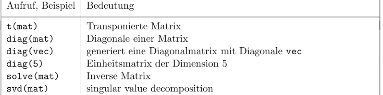
k Matrix-Funtionen. S enth¨alt alle wichtigen Funktionen f¨ur lineare Algebra. Eine Aus- wahl zeigt Tabelle ??.
2.6. MATRIZEN 13
Aufruf, Beispiel Bedeutung
t(mat) Transponierte Matrix diag(mat) Diagonale einer Matrix
diag(vec) generiert eine Diagonalmatrix mit Diagonale vec diag(5) Einheitsmatrix der Dimension 5
solve(mat) Inverse Matrix
svd(mat) singular value decomposition
Tabelle 2.6.k: Wichtige Funktionen f¨ur Matrizen
3 Einfache Statistik
3.1 Einfache Statistik-Funktionen
a Hier wollen wir einige Statistik-Funktionen von S vorstellen, die f¨ur grundlegende Pro- blemstellungen wie Ein- und Zwei-Stichproben-Test gebraucht werden.
b Tabellen. Die Funktion tablez¨ahlt, wie oft jeder Wert vorkommt,
> table(d.blast[,"loc"]) L1 L2 L3 L4 L5 L6
14 10 14 10 24 24
Der OrtL1 kam also beispielsweise im Datensatz 14 Mal vor.
c Will man stetige Daten zuerst klassieren, dann ist die Funktioncutn¨utzlich,
> t.speer <− cut(d.sport[,"speer"],seq(50,75,5))
> table(t.speer)
(50,55] (55,60] (60,65] (65,70] (70,75]
3 2 3 6 1
Ahnliches erreicht man – weniger gut lesbar – mit der Funktion¨ hist und Argument plot=FALSE,
> hist(d.sport[,"speer"], plot=FALSE)
(Die Klassengrenzen werden hier gerade gleich gew¨ahlt wie oben!)
d Die Funktion table erstellt auch zweidimensionale Tabellen, so genannte Kontingenzta- feln,
> t.kugel <− cut(d.sport[,"kugel"],seq(13,17,1))
> table(t.kugel, t.speer) t.speer
t.kugel (50,55] (55,60] (60,65] (65,70] (70,75]
(13,14] 0 0 0 2 0
(14,15] 3 0 0 2 0
(15,16] 0 0 2 2 1
(16,17] 0 2 1 0 0
– nur leider ohne Randsummen und Prozentwerte.
R-Kurs, cSeminar f¨ur Statistik
3.2. TESTS 15
e Numerische Beschreibung.
Sch¨atzung eines
”Lokations-Parameters“:
> mean(x) ; median(x) Varianz: var(x)
Korrelation:
> cor(d.sport[,"kugel"], d.sport[,"speer"]) [1] -0.146
Korrelations-Matrix:
> t.cor <- cor(d.sport[,1:3])
> round(100*t.cor) weit kugel hoch
weit 100 -63 34
kugel -63 100 -9
hoch 34 -9 100
3.2 Tests
a Tests und Vertrauensintervalle. F¨ur Tests und Vertrauensintervalle f¨ur den Parame- ter der Binomial-Verteilung ist die Funktion binom.testda:
> binom.test(3,20, p=0.4)
gibt ein ausf¨uhrliches Resultat mit P-Wert des Tests auf π= 0.4 und mit einem Vertrau- ensintervall.
b F¨urzwei unabh¨angige Stichprobenliefert wilcox.testdie Resultate des Rangsum- mentests und t.testdiejenigen des t-Tests,
> t.hh <− d.sport[,"hoch"]>200
> t.kugel <− d.sport[,"kugel"]
> wilcox.test(t.kugel[t.hh],t.kugel[!t.hh]) Wilcoxon rank sum test
data: t.kugel[t.hh] and t.kugel[!t.hh]
W = 20, p-value = 0.4559
alternative hypothesis: true mu is not equal to 0
> t.test(t.kugel[t.hh],t.kugel[!t.hh], var.equal = TRUE) Two Sample t-test
data: t.kugel[t.hh] and t.kugel[!t.hh]
t = -0.8066, df = 13, p-value = 0.4344
alternative hypothesis: true difference in means is not equal to 0 95 percent confidence interval:
-1.694 0.773
16 3 EINFACHE STATISTIK
sample estimates:
mean of x mean of y
15.01 15.47
F¨ur gepaarte Stichproben oder eine einzelne Stichprobe liefern die gleichen Funktionen mit dem Argumentpaired=TRUEdie Resultate.
3.3 Modell-Formeln
a Ein wesentlicher Teil der Statistik befasst sich damit, Zusammenh¨ange zwischen Variablen zu untersuchen. In der statistischen Regressions- und Varianzanalyse werden dazu Modelle aufgestellt. Um solche Modelle f¨ur die Software festzulegen, gibt es eine eigene ”Sprache“
oder Syntax, die nicht nur in der S-Sprache verwendet wird.
Diese Formel-Sprache kann auch dazu ben¨utzt werden, grafische Darstellungen zu verlan- gen. Wir f¨uhren sie deshalb schon hier ein – wenigstens die einfachsten
”Ausdr¨ucke“, lange bevor wir auf die eigentlichen Modelle zu sprechen kommen.
b Eine einfache Formel sieht so aus:
kugel ∼ speer + weit
Jede Formel enth¨alt das Zeichen ‘∼’ (Tilde). Links davon steht die Zielvariable (kugel), rechts stehen die
”Eingangs-Variablen“ (speer,weit) des Modells. In Streudiagrammen wird die Zielvarible schliesslich vertikal, die Eingangs-Variablen werden horizontal aufge- tragen. Die einzelnen Variablen auf der rechten Seite werden durch ein ‘+’ voneinander getrennt – obwohl hier keine Variablen zusammengez¨ahlt werden.
Mehr ¨uber Formeln folgt im Kapitel ¨uber Regression.
c Eine Formel kann auch in der ¨ublichen Weise abgespeichert werden. Sie bleibt eine Formel, also eine Art Satz in der Formel-Sprache. Erst wenn sie einer Funktion ¨ubergeben wird, die damit etwas anfangen kann, werden daraus wieder Werte von Variablen, also konkrete Zahlen.
d Ein Beispiel einer solchen Funktion ist plot:
> plot(kugel ∼ speer, data=d.sport)
!!!
4 Graphics
4.1 Overview
a Several R graphics functions have been presented so far:
> plot(d.sport[,"kugel"], d.sport[,"speer"], + xlab="ball push", ylab="javelin", pch=7)
> plot(punkte ∼ kugel+speer, data=d.sport)
> pairs(d.sport)
> boxplot(sleep[1:10,"extra"],sleep[11:20,"extra"],ylab="extra") Many more functions are available and will be introduced:
scatter.smooth(),matplot(),image(), ...
lines(),points(), . . .
par(),identify(),dev.new(), . . .
b There are 6 kinds of R graphics functions:
• High-level plotting functions such as plot()
⇒generate a new graphical display of data.
• Low-level plotting functions such as lines()
⇒add further graphical elements to an existing graph.
• “Interactive” functions such as identify()
⇒enhance or collect information interactively from a graph.
• “Control” functions such as par()
⇒control the appearance of graphs.
• “Device” control functions such as dev.new()
⇒to manipulate windows and files that display or store graphs.
4.2 Scatterplot
a The most common graphical display shows the values of two variables, plotted against each other. The (first) syntax is
> plot(x=x, y=y, main="...", xlab="...", ylab="...", ...)
x,y are two numeric vectors.
Example:
> plot(x=meuse[,"x"], y=meuse[,"y"], xlab="easting", ylab="northing", + main="sampling locations")
R-Kurs, cSeminar f¨ur Statistik
18 4 GRAPHICS
b Three alternative ways to invoke plot():
• Plot of the values of a single vector against the position indices of the vector elements:
> plot(meuse[,"zinc"], ylab = "zinc")
• Scatterplot of two columns of a matrix or a dataframe
> plot(meuse[,c("x","y")])
• Use of a model “formula” to select y and xvariable from a data frame:
> plot(zinc∼dist, data=meuse)
Note: y∼x: The variable to be used on the vertical axis comes first.
c Many argumentsof plot()arecommonto many graphics functions:
• main="...",xlab="...",ylab="...", where ...: any character string
⇒ used to set titleand labelsof axes
• log="x",log="y",log="xy"
⇒ forlogarithmic scaling of axes
• xlim=c(xmin,xmax),ylim=c(ymin,ymax)
⇒ setranges for the values to be displayed.
• asp=n
⇒ set “aspect ratio” of axes, i.e. ratio of lengths of “measurement” units on y and x axis. This is most often used to ensure that the scales of both axis are equal when displaying a geographical location or two geometrical measurements of an object, by setting asp = 1.
• pch=i or pch="c"
⇒ select the plotting symbol(s) c: a (vector of) single character(s) or
i: a (vector of) integer(s) to select one of the built-in geometrical symbols (square, cricle, triangle, cross, ..., see?points for a list).
If a vector is given, different symbols will be used for the different points (recycled if necessary).
• cex=n
⇒ choose the size of the symbols, relative to the standard size that the plot function would choose by default. A vector can be given as with pch.
• col=i or col="color"
⇒ choose thesizeand colorof symbols
color: name of color in english (col = "red"). A vector can again be given as with pch.
4.3. BOXPLOT 19
4.3 Boxplot
a Boxplots show the most important aspects of (the distribution of) a sample in a simple way. Syntax:
> boxplot(x=x, notch=l, horizontal=l, ...)
notch = TRUE: “notches” are added to roughly test whether two medians are significantly different
horizontal = TRUE: boxplots are shown horizontally. (There is no argument vertical.) Example:
> boxplot(x=meuse[,"zinc"], notch=TRUE, horizontal=TRUE, log="x", + xlab="zinc content")
b Variations of boxplots:
• Boxplot of several variables in same graph:
> boxplot(meuse[,c("zinc","lead")], horizontal=TRUE, log="x")
• Boxplots of several groups for one variable:
> boxplot(zinc∼ffreq, data=meuse)
4.4 Adding Points and Lines to a Plot
a Use points() to add further points to a graph created before by a high-level graphics function.
> points(x=x, y=y, pch=i, col= , cex=n, ...) Example:
> plot(lead∼dist.m, data=meuse, ylim=c(10,1000), log="y")
> points(meuse[,c("dist.m","copper")], + col="red", pch=3)
b Lines can be added bylines() to a graph.
> lines(x=x, y=y, col= , lty= , lwd=n,...) lty=i or lty="linetype"(keyword): type of line n: line width relative to default value
Example:
> plot(y∼x, meuse, asp=1)
> lines(meuse.riv, lty="dotted", lwd=2.5, col= "cyan")
c Straight linesthrough the whole plotting area can be added by abline()to a graph.
> abline(a=n, b=n, h=v, v=v, ...)
Provide either values to a(intercept) andb(slope) or h=v as the (y) position(s) of hori- zontal orv=v as the (x) position(s) ofvertical straight line(s).
Example:
> plot(lead∼dist.m, meuse, asp=1)
> abline(h=c(200,500), lty="dotted", col=c("orange","red"))
> abline(a=300, b=-1, lty="3313", lwd=3)
20 4 GRAPHICS
d Line segmentsare added by segments().
> segments(x0=v, y0=v, x1=v, x2=v, ...)
Line segments are drawn from the points(x0,y0) to the points (x1,y1) (v numeric vectors of same length).
Example:
> plot(y∼x, meuse)
> t.xr <- range(meuse[,"x"])
> t.yr <- range(meuse[,"y"])
> segments(x0=rep(t.xr[1],2), y0=t.yr, x1=rep(t.xr[2],2), y1=t.yr[2:1] ) e Polygons are added bypolygon().
> polygon(x=x, y=y, density=n, angle=n, border= , col= ,...)
Provide values todensityand angleforhachuring and to borderandcol forborder and fill colorof polygons. ???
Example:
> plot(y∼x, meuse, asp=1)
> polygon(meuse.riv, border="blue", col="cyan", angle=135, density=10)
4.5 Adding Text to a Plot
a Pointsin a scatterplot arelabelledbytext().
> text(x=x, y=y, labels= , pos=i, ...)
Provide a vector of character strings to labels. The argumentpos controls whether the text is plotted below (1), to the left (2), above (3) or to the right (4) of the points.
Example:
> plot(y∼x, meuse, asp=1, type="n")
> text(meuse[,c("x","y")], cex=0.7, labels=meuse[,"landuse"])
b Legend. Place a legend explaining any different symbols or line types used bylegend().
> legend(x= , y=n, xjust=n, yjust=n, legend= , col= , lty= , pch= ,...)
The position of the legend is either specified byxandyin combination with the arguments xjust, yjust or by a keyword such as "bottomleft" as the first argument (cf.?legend for details). legend contains the explanatory text as a vector of character strings. One or more of the remaining arguments will be specified by a vector of the same length as legendand will give the symbols and line types (pchandlty), the symbol sizes (cex), or the colors (col).
Example:
> plot(meuse[,c("x","y")], asp=1, col=as.numeric(meuse[,"ffreq"]), + cex=sqrt(meuse[,"zinc"])/10)
> legend(x="topleft", pch=c(NA,rep(1,3)), + col=c("black","black","red","green"),
+ legend=c("flooding", "often", "intermediate", "rarely"))
4.6. INTERACTING WITH A PLOT 21
4.6 Interacting with a Plot
a Pointsin plots are identified and querried interactively byidentify().
> identify(x=x, y=y, labels= )
Provide a character or numeric vector of the same length asxandytolabelsfor labelling identified points accordingly. Click the right hand mouse button to stop identifying.
Example:
> plot(meuse[,c("x","y")], asp=1, cex=sqrt(meuse[,"zinc"])/10))
> t.i <- identify(meuse[,c("x","y")], labels=meuse[,"zinc"])
Now, the sequence numbers of the identified points are available as t.ifor further use.
b Read the coordinates of interactively selected points from plots by usinglocator().
> locator(n=i, type="p")
You can either specify the number i of points to locate in advance or right-click to stop locating points.
Example:
> plot(meuse[,c("x","y")], asp=1)
> polygon(locator())