The Sun’s Role in Climate Variations

(1)

R E V I E W : C L I M A T O L O G Y

The Sun’s Role in Climate Variations

D. Rind

Is the Sun the controller of climate changes, only the instigator of changes that are mostly forced by the system feedbacks, or simply a convenient scapegoat for climate variations lacking any other obvious cause? This question is addressed for suggested solar forcing mechanisms operating on time scales from billions of years to decades.

Each mechanism fails to generate the expected climate response in important respects, although some relations are found. The magnitude of the system feedbacks or variability appears as large or larger than that of the solar forcing, making the Sun’s true role ambiguous. As the Sun provides an explicit external forcing, a better understanding of its cause and effect in climate change could help us evaluate the importance of other climate forcings (such as past and future greenhouse gas changes).

How much the climate system is influenced by solar variability has long been a subject of controversy, due largely to the strictly empirical nature of the evidence. Observations of past or current climate have been correlated with presumed variations of solar irradiance or solar activity proxy records, and a de facto cause and effect relation has been established.

For those convinced of the Sun’s dominance, this is generally sufficient. For critics, the correlations often do not extend sufficiently long to establish statistical significance; noth- ing suffices short of complete understanding of how the energy associated with solar variability produces the responses at each step of the process. Rarely is the latter achieved for any forcing of the climate system, even when physical relations are apparent (witness the search for the smoking gun of anthropogenic greenhouse warming). Empirical correlations do not necessarily imply causation, especially when the climate data quality and dating is imperfect and solar forcing is poorly known.

However, the sheer number of empirical Sun- climate relations defies ready dismissal.

One difficulty is that different sides typi- cally adopt absolutist views of the problem:

either the Sun is responsible in a dominant way or it is of no consequence whatsoever.

The reality is that Earth’s atmosphere, land surface, and oceans are not passive recipients of any forcing, be it solar variability, volcanic eruptions, or altered greenhouse gas concentrations. Rather, the entire interconnected system participates in the final climate out- come via multiple, nonlinear feedbacks that can amplify or diminish climate forcing as well as change the nature and consistency of the response. To appreciate the solar effect, we need to disentangle the contributions

made by system feedbacks, natural variability and other forcings. Here, I review the solar variations and climate system response for a range of time scales. Without more progress, such separation will likely occur only by observing the response to increased greenhouse gases.

Eons and the Faint Sun Paradox The concept is well established that the Sun was 25 to 30% less luminous 4.5 Ga, which

should have produced a completely ice- covered Earth for some 2 Gy (1). Yet free flowing water and the beginnings of life were apparent 3.5 to perhaps more than 4 Ga (the “faint Sun paradox”). Large amounts of greenhouse gases are presumed to have been present in the atmosphere to offset the solar deficit, although it is not understood precisely which gases. If it were reducing gases, such as CH₄ or NH₃, or- ganic mixing ratios would be three orders of magnitude more easily generated by lightning discharges, than if it were CO₂

(2). But the Sun’s ultraviolet (UV) radiation would destroy the reducing gases in short order (3). Regardless of the ultimate answer, it is apparent that what would have been expected from solar forcing alone was not what the climate system registered, due presumably to even greater forcings or feedbacks such as altered greenhouse gas concentrations. A comparison of what should have happened if solar forcing were to predominate versus what did happen is given in Table 1.

Conversely, by some 700 Ma the solar reduction of 6% would not have been expected to produce an ice-covered Earth [which in one model seemed to require some 10 to 15%

reduction (4,5)], and yet evidence of ice on equatorial land masses exists for that and other such time periods (6). Now explana- tions are required for the magnitude of the low-latitude cooling, and they range from possible high obliquity (7) to reduced greenhouse gases (8, 9) in conjunction with seren- dipitously arranged continents (10). Again, the magnitude of solar irradiance was not

unimportant and may even have triggered the system responses that eventually led to the observed state, but ultimately it was also not the dominating factor. What else may have happened is shown in Table 1 as well.

Millennia and Orbital Variations Though not normally thought of as “solar variability,” orbital variations force climate by altering the solar input (albeit with variable percentage as a function of latitude) and uniform spectral irradiance change. Because of the prevalence in numerous climate NASA Goddard Institute for Space Studies (GISS) at

Columbia University, 2880 Broadway, New York, NY 10025, USA. E-mail: drind@giss.nasa.gov

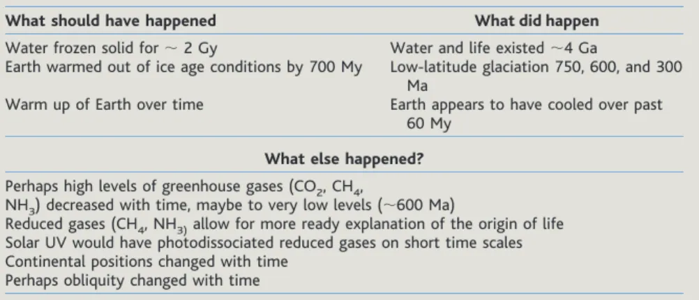
Table 1.Faint Sun paradox. Time scale, age of Earth; mechanism, solar evolution, irradiance increases by 25 to 30% over 4.5 Gy. Forcing, 100 W m^-2.

What should have happened What did happen

Water frozen solid for⬃2 Gy Water and life existed⬃4 Ga

Earth warmed out of ice age conditions by 700 My Low-latitude glaciation 750, 600, and 300 Warm up of Earth over time Earth appears to have cooled over pastMa

60 My What else happened?

Perhaps high levels of greenhouse gases (CO₂, CH₄,

NH3) decreased with time, maybe to very low levels (⬃600 Ma)

Reduced gases (CH₄, NH₃₎allow for more ready explanation of the origin of life Solar UV would have photodissociated reduced gases on short time scales Continental positions changed with time

Perhaps obliquity changed with time

SC I E N C E’S CO M P A S S ^● R E V I E W

(2)

records of cycles near 23, 40, and 100 ky corresponding to precession, obliquity, and eccentricity cycles, respectively, in the Earth’s orbit about the Sun, orbital variations have been called the ‘pacemaker of the ice ages‘ (11). They are a prime example of the

presumed solar dominance of climate on Earth during the past several My. Following the standard assumption that irradiance variations at high northern latitudes during summer cause ice sheets to wax and wane, pre- sented in Table 2 is an assessment of what should have happened with respect to orbital variations, versus what did happen. As in the previous two examples, the climate system has displayed a surprising amount of inde- pendence of the forcing.

Considerable evidence of the 40- and 23- ky cycles in the paleorecord extends back in time for hundreds of millions of years (12).

These solar variations do appear to influence the climate in a (temporally) linear fashion.

However, the big climate changes, associated with the ⬃100-ky cycle (or before 1 My, 450-ky cycle), appear mismatched with the small solar irradiance variations due to eccentricity (⬍0.7 W m^–2 over the past 5 My).

Proposed mechanisms rely on the feedbacks of the climate systems to amplify the solar forcing, although some reports have gone so far as to suggest that the 100-ky cycle may be

completely due to ice sheet instabilities and lithosphere deformation, as deglaciation pro- ceeds through nonlinear interactions between the ice sheets, oceans, and lithosphere with little direct solar influence (13,14) (Table 2).

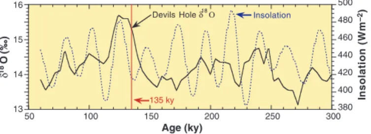
The inappropriateness of solar forcing for the 100-ky cycle has been suggested by observations imply- ing the previous deglaciation was essentially complete by 135 ky (15–17) [e.g., Fig. 1 (18)], when solar irradiance was still low. The match between the paleorecord and the insolation is also poor for some other time periods, including the well-known discrep- ancy between 350 to 450 ka when a full glacial cycle has no corresponding insolation extremes. Computer climate model simulations of the beginning of the last ice age have generally shown the solar insolation change was not sufficient (19,20) unless additional, somewhat extreme feedbacks are hypothe- sized, which then lead to ice in inappropriate places (21,22).

Were the Sun completely unimportant, the disappearance of the last ice sheets timed to match increasing solar irradiance during North- ern Hemisphere (NH) summer⬃14 ka (Fig. 2) would be a coincidence. An intermediate sug- gestion would be that at this point in time the solar forcing could have acted to trigger the appropriate ice sheet instability, thus appearing to exert a prevailing influence on the climate.

Alternatively, the solar irradiance and/or ice sheet changes could induce ocean circulation or trace gas changes (CO₂, methane), which would then provide much of the climate forcing and might help explain the lead of the Southern Hemisphere (SH) in some aspects of the glacial cycle. As emphasized by the opposing relations

in Figs. 1 and 2, in a system with many com- peting nonlinear feedbacks a consistent response may be a naı¨ve concept.

Centuries and Total Irradiance Change Solar irradiance has now been monitored for the past 2 decades, and shows peak-to-peak changes on the order of 0.1%. Maximum irradiance occurs during sunspot maxima (23); though the sunspot itself reduces radiation, excess illumination is associated with the faculae, bright regions that surround the sunspots. This has led to attempts to reconstruct irradiance variations during the past millennia on the basis of variable sunspots, either directly observed or inferred from the variations in¹⁴C and¹⁰Be found in the paleorecord. With reduced sunspot activity, Earth’s magnetic field is less disturbed and better shields the atmosphere from the high- energy particles that produce these isotopes.

To produce solar irradiance changes⬎0.1%

requires an additional mechanism when sunspots disappear for long periods of time (such as the Maunder Minimum, between 1645 and 1715), perhaps involving the background activity network on the Sun. Changes for this time period have been estimated in the range of 0.2 to 0.35% (24, 25), similar to those estimated from the difference between cy- cling and noncycling Sun-like stars (26,27).

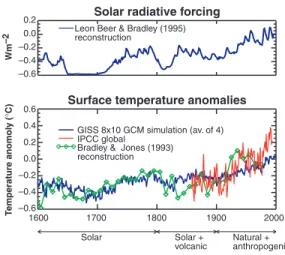
A total irradiance change of such magnitude used to force General Circulation Mod- els (GCMs) produces a global average climate change of some 0.5°C (28–30). With respect to the global mean temperature, a reasonable match with some temperature reconstructions is achieved by models, particu- larly in the preindustrial epoch between 1600 and 1800 (Fig. 3). From this perspective, solar variations dominated climate in preindustrial times. That both the estimated solar irradiance and surface temperatures exhibit overall increases in the 20th century has led some empirical analyses (31) and model results (32) to claim that this dominance has Fig. 1.Well-dated isotopic record from the Devils Hole cave showing the

warming of the penultimate deglaciation essentially finished before the summer insolation at 65°N began to increase. This is in agreement with some other data sources, including the latest temperature reconstructions from the Vostok ice core. [Reprinted from (18) with permission.]

Fig. 2. GISP 2 and Vostok isotopic records, showing the latest deglaciation in phase with summer insolation at 65°N. [Reprinted from (13) with permission.]

Table 2.Orbital variations. Time scale, 2 My; mechanism, solar irradiance at high latitudes during NH summer changes with time due to precession, obliquity and eccentricity variations;

forcing,⬃30 W m^-2at 65°N in summer.

Ice ages with less NH summer irradiance GCMs did not get cold enough Interglacials with more NH summer irradiance Interglacials did not always match

SH responds to NH lead SH led in some responses

Domination of precession and obliquity cycles

at 40 ky,⬃23 ky 100-ky cycle dominated

What else happened?

Possible ice sheet instabilities Possible deep water changes Greenhouse gas (CO2, CH4) changes Dating uncertainties

(3)

extended through the first half of the 20th century (33).

However, a closer look at the observations indicates the climate system has been much more variable than implied by the global mean temperature. There is little consistency in the growth of mountain glaciers during the ‘Little Ice Age‘ (i.e., 1500 –1850 AD), with ice ad- vances at different times that do not necessarily coincide with the reconstructed solar irradiance reductions (34, 35). Nor does the Medieval Warm Period of higher reconstructed irradiance (1000 –1400 AD), show consistency in warming from one region to another (36,37). At the very least, this implies that natural variations or other forcings of the system can override the climate’s response to solar forcing of this (estimated) magnitude for particular regions. In addition, solar forcing of several decades’ du- ration will have less effect on oceans, with their higher heat capacity, than on land, which sets up temperature gradients that lead to wind changes and changes in the advection of heat.

Hence, some regions warm even when the globe cools (29). The failure to find cooling everywhere in conjunction with proposed solar reductions, therefore, does not mean that solar- induced climate changes have not occurred but rather that the system response is neither simple nor direct.

These concepts are highlighted in Table 3, as is a reference to apparent cycles in paleodata, which have also been related to cycles in the Sun. Such climate cycles are continually being reported, with the two most often-noted variations being the Suess (⬃210-year) and Gleiss- berg (88-year) cycles, seen for example in varved sediments (38) and in the isotope record (39). The 210-year cycle has recently been associated with droughts in the Maya lowlands (40) and East Africa (41), possibly influencing the demise of these civilizations. To what do these cycles refer? Are they natural variations within the Sun or natural cycles within the atmosphere-ocean system, either in the Pacific

or the Atlantic (42,43)? (Although why such internal cycles should affect the isotope record corrected for accumulation changes is not obvious.) The Suess cycle has been related to the various astronomical phenomena, such as the angular momentum of the Sun about the center of mass, due to the periods of the four big planets or other orbital effects (44,45), a possibility most solar physi- cists reject. An approximately 1500- year cycle seen in the North Atlantic has been correlated with inferred changes in production rates of¹⁴C and¹⁰Be and, thus, may also be solar driven. This may be possibly amplified by North Atlantic deep water changes (46), another example of how feedbacks might signif- icantly alter the nature of the climate response.

Decades and Spectral Irradiance Change

Many atmospheric phenomena exhibit decadal variability on both regional and global scales. Such phenomena have often been related empirically to solar cycle variations, on the order of 11 or sometimes 22 years (43, 47,48). In some cases, the relation appears energetically realistic, in ocean temperatures

(49), for example. However, in many instanc- es, problems arise in establishing the physical link between the small magnitude of the forcing and the alleged response.

One possible explanation involves solar UV irradiance variations (50) affecting ozone, which then changes the temperature and wind patterns in the stratosphere, modulating planetary wave energy propagating from the tropo- sphere. This, in turn, alters tropospheric planetary wave energy, wind and temperature advection, and a host of other climate phenomena.

Observations (51) and GCM studies with sufficient coverage of the Middle Atmosphere (52, 53) have converged on a number of these fea-

tures, and its reality is becoming more firmly if not completely verified. This mechanism has also been modeled for multidecadal time scales, such as the Maunder Minimum, and found to result in higher pressure near the pole [the negative phase of the Arctic Oscillation (AO)]

(54,55).

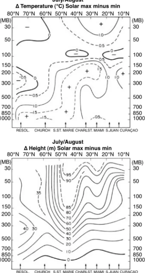
However, on both the decadal and century time scales, the planetary wave response cannot explain important components of the observations (Table 4). Shown in Fig. 4 (56,57) are the solar maximum minus solar minimum temperatures and heights during NH summer at various locations. This effect has not been duplicat- ed in GCMs; in summer, planetary wave energy is smaller and the prevalence of east winds in the stratosphere further minimizes planetary wave influence. On the longer time scale, the Little Ice Age growth of glaciers in Western Europe is similarly unexplained by this mechanism alone. These glaciers respond to winter mass balance (snow accumulation) and summer temperatures (58). The AO [or the North At- lantic Oscillation (NAO)] has little direct ex- pression during summer, and the negative phase produces negative mass balances for these glaciers during winter (58). In the GISS GCM, the negative phase also depends on substantial tropical cooling, which is not evident in the latest temperature reconstructions (59–62).

What else may have happened is indicated in Table 4. Eleven- or 22-year cycles have been related to internal mechanisms in the climate system, specifically anomalies in the ocean (42, 43). Conceivably, these may be related to solar-induced variations, affecting either the surface wind field or deep-water production for the Little Ice Age. Other atmospheric mechanisms may be responding to solar forcing, such as the low-latitude Hadley Cell (63), although the energy mismatch be- Fig. 3.Estimated solar radiative forcing (top) and global surface temperature anomalies, from both GISS model simulations (29) and observations. One canonical view is that solar forcing provides a good match for the observations before 1800, volcanic forcing becomes important during the 19th century, and anthropogenic forcing begins dominating during the 20th century.

[Figure courtesy of J. Lean.]

Table 3.Total solar irradiance variations. Time scale, decades to centuries; mechanism, total solar irradiance changes, possibly in cycles, due to variations in active regions on the Sun alter

Earth’s radiative balance; forcing, 1 W m^-2.

Reduced irradiance with reduced (sunspot)

activity Inconsistent climate correlations with sunspots

Global warming (cooling) with increased

(decreased) solar activity Neither warming nor cooling is ubiquitous or synchronous

No externally driven activity cycles in the

Sun Unclear whether apparent cycles in paleodata

related to periods of big planets What else happened?

Solar irradiance estimated changes may be wrong

Advective temperature changes may overwhelm radiative forcing Climate observations may be inadequate

Natural variations (cycles) may dominate

(4)

tween the small solar input and the latent heat release driving tropical cells would require some especially sensitive catalytic compo- nent. Or the forcing due to solar cycle variations may be by some other means.

Variability and Geomagnetic Activity Another characteristic of solar variability is fluctuations of plasma in the Sun-Earth space

environment. Emitted solar protons, energetic electrons in the magnetosphere, and the interplanetary magnetic field all vary as a result of the basic solar magnetic dynamo that drives the 11-year cycle. Galactic cosmic ray (GCR) intrusions into the lower atmosphere respond to variations in Earth’s magnetic field induced by its coupling with the interplanetary magnetic field and perturbations by eruptive solar events that propagate via the solar wind.

One aspect that has intrigued researchers is the possibility of charged particles acting as cloud condensation nuclei. If clouds are affect- ed, the reasoning goes, significant impacts would undoubtedly follow because the clouds would alter the radiation balance of the atmosphere, altering climate (64). A presumed relation between clouds in specific regions and measures of solar activity is shown in Fig. 5 (64). High geomagnetic activity is thought to influence galactic cosmic rays, hence cloud condensation nuclei, and produce an increase in clouds when solar activity is low (allowing more cosmic rays to enter Earth’s atmosphere).

The expectation and result associated with this mechanism is discussed in Table 5. The response should maximize at high latitudes where the input of GCRs (which enter Earth’s

atmosphere primarily along its polar magnetic field lines) due to solar variability is greatest, but in the observations analyzed it actually was largest at low latitudes (65). The GCR or the cloud response is not consistent with time; ex- tending the record forward to the latter part of the 1990s produces no systematic change from the mid 1990s (66).

As noted in Table 5, the low-latitude phenomena may be responding to other things such as El Nino–Southern Oscillation (ENSO) changes (67). Our understanding of the influence of particle phenomena on the neutral atmosphere is not great, and subtle influences could be operative without our ability to ob- serve them. Alternatively, the cloud cover variations may be driven by a different solar-induced mechanism such as changing UV radiation affecting the atmospheric circulation (68).

Conclusions

The common denominator among an array of potential solar forcing mechanisms operating on a wide range of time scales is that they all are interacting with system feedbacks or variability that may be stronger than the forcing

Fig. 4.Temperature and height differences between four solar maximum and solar minimum conditions during July and August at various stations between 65°W and 95°W. GCM simulations cannot reproduce the magnitude of this effect. More than 40% of the interannual temperature variance during this season is associated with the 11-year cycle (57). [Reprinted from (56) with permission.]

Fig. 5.Changes in cloud cover compared with the variation in cosmic ray fluxes (solid curve) and 10.7 cm solar flux (broken curve). Data is from Nimbus 7 and Defense Meteorogical Sat- ellite Program (DMSP) (SH over oceans) and International Satellite Cloud Climatology Project (ISCCP) over oceans with the tropics excluded. All data smoothed with a 12-month running mean. [Reprinted from (64) with permission.]

Table 4.Solar cycle spectral variations. Time scale, 11 years, possibly decades; mechanism, small solar UV variations affect ozone, stratospheric temperatures and winds, and propagation of tro-

pospheric planetary waves (may affect natural atmospheric modes); forcing, 0.3 W m^-2.

Effects propagate down from

stratosphere Downward propagation seen in observations but not in most GCMs

Effects much stronger in winter Solar cycle effects also strong in summer Multidecadal AO–NAO phase change

depends on significant tropical response

Tropical response uncertain on expected time scales

What else happened?

Solar forcing may be by some other mechanism

Other atmospheric processes may be involved (e.g., Hadley Cell)

Climate forcing may be by some other mechanism (e.g., ocean circulation anomalies) with or without solar involvement

Table 5.Geomagnetic activity. Time scale, 11 years, possibly decades or more; mechanism, variations in relativistic electrons, solar wind, and galactic cosmic rays affect climate via changes in

cloud formation; forcing magnitude uncertain.

Cloud condensation nuclei increase with

greater ionization Real world effects uncertain

Increased low level clouds affect climate Relation of clouds to solar cycle inconsistent with time Response maximizes at high latitudes Low level cloud effects greater at

low latitudes What else happened?

Apparent low cloud effect may be due to other phenomena (e.g., ENSOs, natural variability, short data record)

Apparent cloud effect may be due to other solar mechanisms (UV-induced circulation changes)

(5)

itself. Ironically, this is true even for earlier time periods when the solar forcing was much larger. This state of affairs helps explain why potential Sun-climate relations are controversial and difficult to prove. It also implies that even if the solar forcing could be predicted, the response would still be uncertain due to our present incomplete understanding of climate system feedbacks and internal oscillations. There is no doubt that there are some clear signatures of solar forcing in the system, including some of the orbital variations and planetary wave–mean flow interactions and possibly total irradiance variations. Whether the Sun acts as the controller of climate changes on various time scales, simply instigates the subsequent feedbacks that then dominate the observed record, or is only a convenient explanation for unob- served forcings or system oscillations, will probably be a matter of debate and continued investigation for many years. The answer may also bear on whether the continued growth of atmospheric trace gases will dominate the system response or whether it too will be swamped by the feedbacks, making predictions of any response equally difficult.

References and Notes

1. C. Sagan, G. Mullen,Science177, 52 (1972).

2. C. F. Chyba, C. Sagan,Nature355, 125 (1992).

3. W. R. Kuhn, S. K. Atreya,Icarus37, 207 (1979).

4. M. Chandler, E. Sohl,Eos20Spring Meeting Suppl.

abstr. U22A-06 (2001).

5. W. T. Hyde, T. J. Crowley, S. K. Baum, and W. R. Peltier [Nature405, 425 (2000)] show that using the appropriate solar reduction by itself appears to result in open water (which may actually have existed).

6. P. F. Hoffman, A. J. Kaufman, G. P. Halverson, D. P.

Schrag,Science281, 1342 (1998).

7. D. M. Williams, J. F. Kasting, L. A. Frakes,Nature396, 453 (1998).

8. G. S. Jenkins, S. Smith,Geophys. Res. Lett.26, 2263 (1999.)

9. M. A. Chandler, E. Sohl,J. Geophys. Res.105, 20737 (2001).

10. T. R. Worsley, D. L. Kidder,Geology19, 1161 (1991).

11. J. D. Hayes, J. Imbrie, N. J. Shackleton,Science194, 1121 (1976).

12. See, for example, T. D. Herbert, J.S. Gee, S. D. Donna, inLate Cretaceous Climates, E. Barrera and C. John- son, Eds., (Soc. Sediment. Geol., Tulsa, OK, Spec. Vol.

322, 1999) pp. 105-120.

13. This possibility is reviewed by P. U. Clark, R. B. Alley, and D. Pollard [Science286, 1104 (1999)].

14. J. C. Zachos, N. J. Shackleton, J. S. Revenaugh, H. Palike, and B. P. Flower [Science292, 274 (2001)] find⬃100- ky cycles in addition to the 400-ky cycles some 22 My ago. This implies that these cycles are not necessarily associated with ice sheet dynamics, or alternatively that they can be triggered throughout the climate system by variations of ice on Antarctica.

15. G. Henderson, N. Slowey,Nature404, 61 (2000).

16. C. D. Gallup, H. Cheng, F. W. Taylor, R. L. Edwards, Science295, 310 (2002).

17. J. Levine, D. B., Karner and R. A. Muller, [Eos82(47) (Fall Meeting Suppl.) abstr. U12A-0004 (2001)] reviewed additional evidence showing warming to current Holocene values by 140 ka at some 20 ocean data points, occurring in all the ocean basins.

18. D. B. Karner, R. A. Muller,Science288, 2143 (2000).

19. D. Rind, G. Kukla, D. Peteet, J. Geophys. Res.94, 12851 (1989).

20. J. F. B. Mitchell,Philos Trans. R. Soc. London B341, 267 (1993).

21. R. G. Gallimore, J. E. Kutzbach, Nature381, 503 (1996).

22. R. W. Peltier [Eos82(47) (all Meeting Suppl.) abstr.

U11A-03 (2001)] suggests that one must include isostatic effects and a more sophisticated ice model to improve the chances of getting ice to grow.

23. C. Frohlich, J. Lean, Geophys. Res. Lett.25, 4377 (1998).

24. D. V. Hoyt, K. H. Schatten,J. Geophys. Res.98, 18895 (1993).

25. J. Lean,Geophys. Res. Lett.27, 2423 (2000).

26. S. Baliunas, R. Jastrow,Nature348, 520 (1990).

27. R. R. Radick, G. W. Lockwood, B.A. Skiff, S. L. Baliunas, Astrophys. J. Suppl. Ser.118, 239 (1998).

28. U. Cubasch, R. Voss, G. C. Hergel, J. Waszkewitz, T.

Crowley,Clim. Dyn.13, 757 (1997).

29. D. Rind, J. Lean, R. Healy,J. Geophys. Res.104, 1973 (1999).

30. This is a change relative to the current climate due to solar irradiance variation alone. When the effects of atmospheric trace gas and aerosol changes and the combined impact of solar and anthropogenic effects on ozone are included, the GISS Global Climate–

Middle Atmosphere model produces a cooling of some 1.5°C for the late 1600s relative to today [D.

Rind, P. Lonergan, J. Lean, D. Shindell, in preparation].

31. E. Friis-Christensen, K. Lassen, Science 254, 698 (1991).

32. P. A. Scottet al. Clim. Dyn.17, 1 (2001).

33. The degree to which solar variability has dominated the warming of the 20th century is a question of considerable interest. In the Hoyt and Schatten reconstruction (24), the variation of solar intensity is related to solar cycle length, which then implies a strong increase in solar irradiance between 1890 and 1940, as well as in the last few decades. As discussed in Lean (25), the latter result is inconsistent with the 10.7-cm flux and faculae variation, and also an independent estimate based on interplanetary magnetic field variations. The reconstruction in Lean does not use solar cycle length, and when input to a climate model, results in less solar influence during this century.

34. P. D. Jones, R. S. Bradley, inClimate Since A.D. 1500, R. S. Bradley, P. D. Jones, Eds. (Routledge, London, 1992), pp. 649-665.

35. B. H. Luckman, in Climatic Variations and Forcing Mechanisms of the Last 2000 Years, P. D. Jones, R. S.

Bradley, J. Jouzel, Eds. (Springer-Verlag, Berlin, 1994), pp. 85-108.

36. M. K. Hughes, H. F. Diaz, Clim. Change 26, 109 (1996).

37. R. S. Bradley,Science288, 1353 (2000).

38. J. D. Halfman, T. C. Johnson,Geology16, 496 (1988).

39. M. Stuiver, T. F. Braziunas,Holocene3, 289 (1993).

40. D. A. Hodell, M. Brenner, J. H. Curtis and T. Guilder- son,Science292, 1367 (2001).

41. D. Verschuren, K. R. Laird, B. F. Cumming,Nature410, 403 (2000).

42. S. R. Hare and R. C. Francis,Can. Spec. Publ. Fish Aquat. Sci121, 357 (1995).

43. R. Kerr,Science288, 1984 (2000).

44. R. W. Fairbridge, H. J. Haubold, G. Wiondelius,Earth Moon Planets70, 179 (1995).

45. I. Charvatova,Surv. Geophys.18, 131 (1997).

46. G. Bondet al.,Science294, 2130 (2001).

47. See for example J. R. Herman and R. A. Goldberg in Sun, Weather and Climate[Dover Publications, 1985, 360 pp., originally published as NASA SP-426, GPO, Washington, D. C.] for a summary of the myriad correlations established over the years.

48. J. M. Mitchell Jr., C. W. Stockton, and D. M. Meko [in Solar Terrestrial Influence on Weather and Climate, B. M. McCormac and T. A. Seliga, Eds. (D. Reidel, Dordrecht, 1979), pp. 125-143] provided the most publicized relation of the 22-year cycle with climate:

droughts in the western United States. The solar magnetic field switches direction every 11 years, which gives a 22-year cycle (called the Hale cycle) to various solar phenomena.

49. W. B. White, J. Lean, D. R. Cayan, M. D. Dettinger,J.

Geophys. Res.102, 3255 (1997). The mixed layer ocean temperature sensitivity associated with the 11 year cycle in this study,⬃0.1°C/W m², (a conclusion also reached in (59), seems realistic, given that the brevity of the oscillation prevents the sea surface

temperatures, and hence atmospheric feedbacks associated with water vapor, sea ice and perhaps clouds, from fully coming into play.

50. J. Lean [Geophys. Res. Lett.27, 2425 (2000)] reported that UV radiation during recent sunspot cycles varies by 0.39%, and estimated that during the Maunder Minimum it was reduced by some 0.70%.

51. K. Kodera,J. Geophys. Res.100, 14077 (1995).

52. D.T. Shindell, D. Rind, N. Balachandran, J. Lean, P.

Lonergan,Science284, 305 (1999).

53. D. Rind and N. Balachandran [J. Clim.8, 2080 (1995)], as part of a series of articles, were able to simulate some of the observations involving planetary wave propagation changes in conjunction with the solar cycle and the quasi-biennial oscillation (QBO), acting together. While the solar cycle affects the vertical shear of the zonal wind, the QBO affects the hori- zontal shear, and each combination leads to a unique pattern of wave propagation.

54. D. T. Shindell, G. A. Schmidt, M. E. Mann, D. Rind, and A. Waple [Science294, 2149 (2001)] find the negative phase for the AO during the Maunder Minimum.

55. J. Luterbacher, C. Schmutz, D. Gyalistras, E. Xoplaki, and H. Wanner [Geophys. Res. Lett.26, 2745 (1999)]

reconstructed NAO values show a generally negative phase (higher pressure over Iceland) for the entire time period from 1700-1850. This would then not appear to be directly from solar forcing, which is thought to have been relatively high during the 18th century (Fig. 3).

56. K. Labitzke, H. van Loon,J. Clim.5, 240 (1992).

57. H. van Loon, D. J. Shea,Geophys. Res. Lett.26, 2893 (1999).

58. A. Greene, thesis, Columbia University, 2001.

59. M. E. Mann, R. S. Bradley, M. K. Hughes,Nature392, 779 (1998).

60. The issue of the magnitude of tropical cooling during the Maunder Minimum time period is quite controversial, and important as an indication of tropical sensitivity in general. The comparison shown in Fig. 3 was made between the GISS GCM, with a sensitivity of close to 1°C/W m²and an observed temperature reconstruction that indicated about twice as much cooling for the 1650–1700 time period as the reconstruction in (59). The latter produced minimal tropical response, a result which is based upon the utili- zation in creating EOFs of a few widely scattered coral observations, whose ability to reconstruct paleo-temperatures is complicated by salinity effects.

61. L. G. Thompsonet al.[Science269, 46 (1995)] show tropical ice core data that indicates a temperature difference of greater than 1°C (Oˆ¹⁸O⬎1 per mil) between the late 1600s and late 1800s. In contrast, the reconstruction in (59) shows no temperature change between those time periods. That is one reason why (59) shows essentially no correlation between temperature and solar irradiance for the 19th century.

62. Additional questions concerning the tropical temperature reconstruction arise from modeling studies. The simulation discussed in (54), which produced extrat- ropical temperature responses (and AO phase changes) in general agreement with (59) has tropical temperature changes twice as large as those in (59);

without that magnitude of tropical response, the planetary wave refraction and tendency for negative phase of the AO would have been greatly reduced in the model.

63. J. D. Haigh,Science272, 981 (1996).

64. H. Svensmark,Phys. Rev. Lett.,81, 5027 (1998).

65. N. Marsh, H. Svensmark,Space Science Rev.94, 215 (2000).

66. This can be see by accessing the ISCCP total cloud cover, at http://isccp.giss.nasa.gov/climanal1.html 67. P. D. Farrar,Clim. Change47, 7 (2000).

68. P. M. Udelhofen, R. D. Cess,Geophys. Res. Lett.28, 2617 (2001).

69. J. Lean provided invaluable comments in review. J.

Lerner and M. Shopsin helped in the preparation of the figures. Studies of the impact of solar effects on climate are funded by the NASA Living With A Star program, while stratospheric modeling at GISS is funded by the NASA ACMAP program, and climate modeling is funded by the NASA Climate Program Office.