Biogeosciences Discuss.,
https://doi.org/10.5194/bg-2019-64-SC1, 2019
© Author(s) 2019. This work is distributed under the Creative Commons Attribution 4.0 License.
Interactive comment on “What was the source of the atmospheric CO
2increase during the
Holocene?” by Victor Brovkin et al.
Peter Köhler peter.koehler@awi.de
Received and published: 2 May 2019
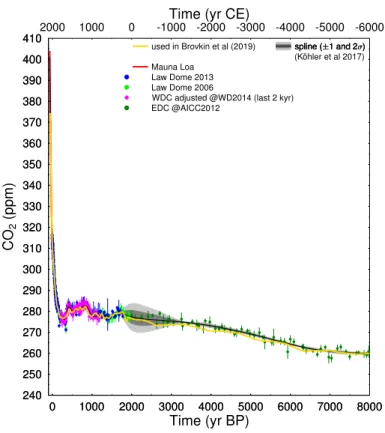
This paper (Brovkin et al., 2019) uses atmospheric greenhouse gases (GHG: CO2, CH4, N2O, plotted in Figure 1b,c of the discussion paper) from spline routines based on various data sets. Since such a GHG data compilation excercise including the calculation of a spline has also been performed in a recent study (Köhler et al., 2017), I asked the corresponding author to get access to their applied GHG time series to evaluate if and how they might differ from the final splines of this other study. I plot them here against these earlier results in the following figures 1–3. Spline routines applied here and there have been the same (developed by Fortunat Joos, Universitiy of Bern), but the underlying data and the chosen prescribed cutoff periodPc for the spline routines have been in detail slightly different leading to similar, but not identical
C1
splines.
For CO2(Fig. 1) both splines are nearly identical.
The CH4(Fig. 2) record inKöhler et al.(2017) is based on the WAIS Divide Ice Core (WDC) for large parts of the Holocene, that resolves multi-cenntennial variabilies, a small-scale featue that is ignored in the spline used inBrovkin et al.(2019). This com- parision also highlights, that the CH4data used inBrovkin et al.(2019) are not global mean values, but southern hemispheric values. Due to an existing interhemispheric gradient, northern hemispheric CH4(e.g. from Greenland ice cores) and therefore also global mean CH4values are slightly larger than the CH4values of the chosen southern hemispheric spline.
In N2O (Fig. 3) the millennial-scale variability is slightly shifted in time between both splines, suggesting that the used age modesl of the underlying data might have been different.
The spline used inBrovkin et al.(2019) fall nearly always into the uncertainty bands (±2σ) of the splines described inKöhler et al.(2017).
For details of the spline method and further citations of the underlying data the reader is refered toKöhler et al.(2017). Layout of figures and captions have been adapted from the previous paper.
I believe these underlying details of the method and data might been of interest to the readers ofBrovkin et al.(2019)
References
Brovkin, V., S. Lorenz, T. Raddatz, T. Ilyina, I. Stemmler, M. Toohey, and M. Claussen (2019), What was the source of the atmospheric CO2 increase during the Holocene?, Biogeo- sciences Discussions,2019, 1–25, doi:10.5194/bg-2019-64.
C2
Köhler, P., C. Nehrbass-Ahles, J. Schmitt, T. F. Stocker, and H. Fischer (2017), A 156 kyr smoothed history of the atmospheric greenhouse gases CO2, CH4, and N2O and their radia- tive forcing,Earth System Science Data,9, 363–387, doi:10.5194/essd-9-363-2017.
Figure Captions
Figure 1: Atmospheric CO2spline and underlying data (2016 CE – 8,000 BP). Black spline as published inKöhler et al. (2017) against time series (gold) used inBrovkin et al.(2019). Error bars around the ice core data points are±2σ. WDC data have been adjusted to reduce offsets, seeKöhler et al.(2017) for details.
Figure 2: Atmospheric CH4 spline and underlying data (2016 CE – 8,000 BP). Black spline as published inKöhler et al. (2017) against time series (gold) used inBrovkin et al.(2019). Details on plotted data are explained inKöhler et al.(2017). The max- imum ice core data uncertainty (±2σ) is sketched in the lower left corner. Latitudinal origin of data is indicated by NH and SH, implying northern and southern hemisphere, respectively.
Figure 3: Atmospheric N2O spline and underlying data (2016 CE – 8,000 BP). Black spline as published inKöhler et al.(2017) against time series (gold) used in inBrovkin et al.(2019). Details on plotted data are explained in in Köhler et al. (2017). The maximum ice core data uncertainty (±2σ) is sketched in the upper right corner. Filled symbols: data taken for spline; open symbols: data not taken for spline.
Interactive comment on Biogeosciences Discuss., https://doi.org/10.5194/bg-2019-64, 2019.
C3
240 250 260 270 280 290 300 310 320 330 340 350 360 370 380 390 400 410
240 250 260 270 280 290 300 310 320 330 340 350 360 370 380 390 400 410
CO2(ppm)
0 1000 2000 3000 4000 5000 6000 7000 8000
Time (yr BP)
0 1000 2000 3000 4000 5000 6000 7000 8000 2000 1000 0 -1000 -2000 -3000 -4000 -5000 -6000
Time (yr CE)
used in Brovkin et al (2019) Mauna Loa
Law Dome 2013 Law Dome 2006
WDC adjusted @WD2014 (last 2 kyr) EDC @AICC2012
spline ( 1 and 2 ) (Köhler et al 2017) spline ( 1 and 2 ) spline ( 1 and 2 )
Fig. 1.Figure caption is contained at the end of text.
C4
300 400 500 600 700 800 900 1000 1100 1200 1300 1400 1500 1600 1700 1800
300 400 500 600 700 800 900 1000 1100 1200 1300 1400 1500 1600 1700 1800
CH4(ppb)
0 1000 2000 3000 4000 5000 6000 7000 8000
Time (yr BP)
2000 1000 0 -1000 -2000 -3000 -4000 -5000 -6000Time (yr CE)
spline ( 1 and 2 ) (Köhler et al 2017) spline ( 1 and 2 ) spline ( 1 and 2 ) used in Brovkin et al (2019)
SH South Pole SH Law Dome, Cape Grim SH WDC discrete OSU @WD2014 SH WDC discrete PSU adjusted @WD2014 for comparison only:
NH GRIP composite @GICC05modelext
2 (max)
Fig. 2.Figure caption is contained at the end of text.
C5
240 250 260 270 280 290 300 310 320 330
240 250 260 270 280 290 300 310 320 330
N2O(ppb)
0 1000 2000 3000 4000 5000 6000 7000 8000
Time (yr BP)
0 1000 2000 3000 4000 5000 6000 7000 8000 2000 1000 0 -1000 -2000 -3000 -4000 -5000 -6000
Time (yr CE)
used in Brovkin et al (2019) NOAA (global mean) Law Dome, Cape Grim EDC @AICC2012 Taylor Glacier @WD2014 Talos Dome @AICC2012
spline ( 1 and 2 ) (Köhler et al 2017) spline ( 1 and 2 ) spline ( 1 and 2 )
2 (max)
Fig. 3.Figure caption is contained at the end of text.
C6