Holocene?” by Victor Brovkin et al.

(1)

Biogeosciences Discuss.,

https://doi.org/10.5194/bg-2019-64-SC2, 2019

Interactive comment on “What was the source of the atmospheric CO

2

increase during the

Holocene?” by Victor Brovkin et al.

Peter Köhler peter.koehler@awi.de

Received and published: 4 May 2019

In the figures of my previous comment the labels of the top x-axes (time in yr CE) are placed wrong, they need to get shifted by 50 years. Furthermore, the x-axes started at -100 yr BP, that has now been changed to -66 yr BP = 2016 CE, which is the first year with data.

I apologize for any confusion, the corrected figures are attached below, including their full captions.

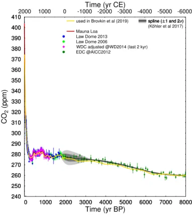
Fig. 1:Atmospheric CO2spline and underlying data (2016 CE to -6050 CE or -66 BP to 8,000 BP). Black spline as published inKöhler et al.(2017) against time series (gold) used inBrovkin et al.(2019). Error bars around the ice core data points are±2σ. WDC

C1

data have been adjusted to reduce offsets, seeKöhler et al.(2017) for details.

Fig. 2: Atmospheric CH4 spline and underlying data (2016 CE to -6050 CE or -66 BP to 8,000 BP). Black spline as published inKöhler et al.(2017) against time series (gold) used inBrovkin et al.(2019). Details on plotted data are explained inKöhler et al.(2017). The maximum ice core data uncertainty (±2σ) is sketched in the lower left corner. Latitudinal origin of data is indicated by NH and SH, implying northern and southern hemisphere, respectively.

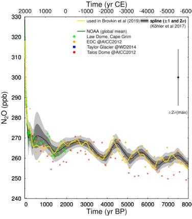
Fig 3:Atmospheric N2O spline and underlying data (2016 CE to -6050 CE or -66 BP to 8,000 BP). Black spline as published inKöhler et al.(2017) against time series (gold) used in inBrovkin et al.(2019). Details on plotted data are explained in inKöhler et al.

(2017). The maximum ice core data uncertainty (±2σ) is sketched in the upper right corner. Filled symbols: data taken for spline; open symbols: data not taken for spline.

References

Brovkin, V., S. Lorenz, T. Raddatz, T. Ilyina, I. Stemmler, M. Toohey, and M. Claussen (2019), What was the source of the atmospheric CO2 increase during the Holocene?, Biogeo- sciences Discussions,2019, 1–25, doi:10.5194/bg-2019-64.

Köhler, P., C. Nehrbass-Ahles, J. Schmitt, T. F. Stocker, and H. Fischer (2017), A 156 kyr smoothed history of the atmospheric greenhouse gases CO2, CH4, and N2O and their radia- tive forcing,Earth System Science Data,9, 363–387, doi:10.5194/essd-9-363-2017.

Interactive comment on Biogeosciences Discuss., https://doi.org/10.5194/bg-2019-64, 2019.

C2

(2)

240 250 260 270 280 290 300 310 320 330 340 350 360 370 380 390 400 410

CO2(ppm)

0 1000 2000 3000 4000 5000 6000 7000 8000

Time (yr BP)

0 1000 2000 3000 4000 5000 6000 7000 8000 2000 1000 0 -1000 -2000 -3000 -4000 -5000 -6000Time (yr CE)

used in Brovkin et al (2019) Mauna Loa

Law Dome 2013 Law Dome 2006

WDC adjusted @WD2014 (last 2 kyr) EDC @AICC2012

spline ( 1 and 2 ) (Köhler et al 2017) spline ( 1 and 2 ) spline ( 1 and 2 )

Fig. 1.Corrected Fig. 1 on CO2 of previous comment C3

300 400 500 600 700 800 900 1000 1100 1200 1300 1400 1500 1600 1700 1800

CH4(ppb)

0 1000 2000 3000 4000 5000 6000 7000 8000

Time (yr BP)

2000 1000 0 -1000 -2000 -3000 -4000 -5000 -6000

Time (yr CE)

spline ( 1 and 2 ) (Köhler et al 2017) spline ( 1 and 2 ) spline ( 1 and 2 ) used in Brovkin et al (2019)

SH South Pole SH Law Dome, Cape Grim SH WDC discrete OSU @WD2014 SH WDC discrete PSU adjusted @WD2014 for comparison only:

NH GRIP composite @GICC05modelext

2 (max)

Fig. 2.Corrected Fig. 2 on CH4 of previous comment C4

(3)

240 250 260 270 280 290 300 310 320 330

N2O(ppb)

0 1000 2000 3000 4000 5000 6000 7000 8000

Time (yr BP)

0 1000 2000 3000 4000 5000 6000 7000 8000 2000 1000 0 -1000 -2000 -3000 -4000 -5000 -6000Time (yr CE)

used in Brovkin et al (2019) NOAA (global mean) Law Dome, Cape Grim EDC @AICC2012 Taylor Glacier @WD2014 Talos Dome @AICC2012

spline ( 1 and 2 ) (Köhler et al 2017) spline ( 1 and 2 ) spline ( 1 and 2 )

2 (max)

Fig. 3.Corrected Fig. 3 on N2O of previous comment C5