JGR: Solid Earth Supporting Information for
Microseismicity and lava flows constrain tectono-magmatic processes near the southern tip of the Fonualei Rift and
Spreading Center in the Lau Basin
F. Schmid1, M. Cremanns1,2, N. Augustin1, D. Lange1, H. Kopp1,2, F. Petersen1
1GEOMAR Helmholtz Center for Ocean Research, Wischhofstraße 1-3, 24148 Kiel, Germany
2Institute for Geosciences, Christian-Albrechts-Universität zu Kiel, Kiel, Germany
Corresponding author: Florian Schmid (fschmid@geomar.de)
Contents of this file
Figures S1 to S6 Tables S1 to S3 12
1 2 3 4 5 6 7
8 9 10 11
12
13
14 15
16
17
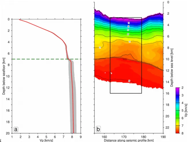
Figure S1. a) The red lines represents the 1D P-wave velocity model used for the location of hypocenters with NonLinLoc and HypoDD. The model was constructed from the 2D refraction seismic P-wave tomography model of Schmid et al. (2020) displayed in panel b. Gray shading represents the
standard deviation of Vp in the tomographic model of Schmid et al. (2020). To achieve the 1D model the velocities inside the black box in panel b were horizontally averaged, after flattening the sea floor. At depths deeper than 15 km below sea level velocities in the 1D model were set to 8.1 km/s. Note, the different reference depths of both panels.
5
6
18
19 20
21 22
23 24
25
26 27
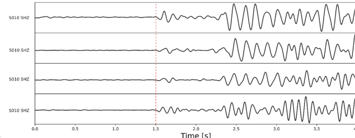
Figure S2. Aligned waveforms recorded by the vertical channel of station S010, originating from four events located in the southern event cluster and occurring within a time window of four hours on the 8th of January 2019. The dashed vertical line marks the P-phase onset. The similarity of the
waveforms, in particular around the P-phase onset, yielded a cross-correlation coefficient larger than 0.85.
9
10
28
29 30
31 32
33
34
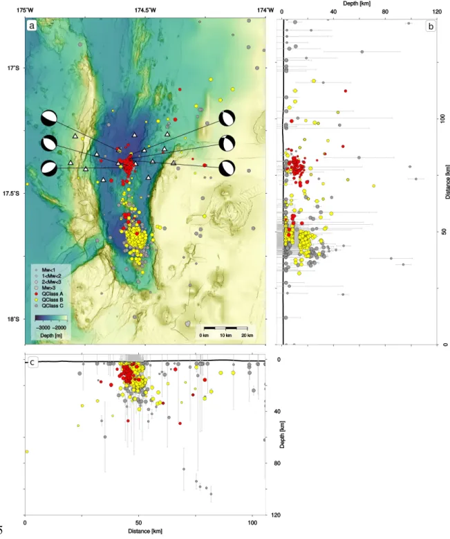
Figure S3. Overview of all 711 NonLinLoc located events, regardless of the location uncertainty. a) Bathymetry map with epicenters color-coded
according to location quality class. White triangles show OBS locations. b) South-North oriented section with projected hypocenters. Gray bars indicate the vertical location uncertainty of individual events. c) West-East oriented transect with projected hypocenters.
13
14
35
36
37 38
39 40
41
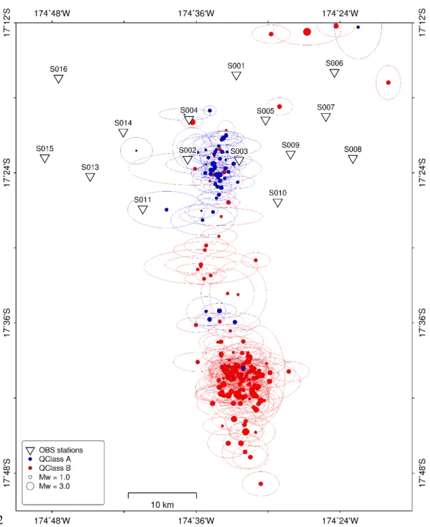
Figure S4. Class A and B events with associated NonLinLoc horizontal location uncertainties represented by ellipses. Note that most events in the southern cluster do not show significantly larger horizontal errors than events below the OBS network. Usually, out-of-network events come with
considerable horizontal location uncertainties. However, in this case events in the southern cluster come with a larger number of phase arrival picks (Figure S5), which compensates for this effect.
17
18
42
43 44
45
46 47
48 49
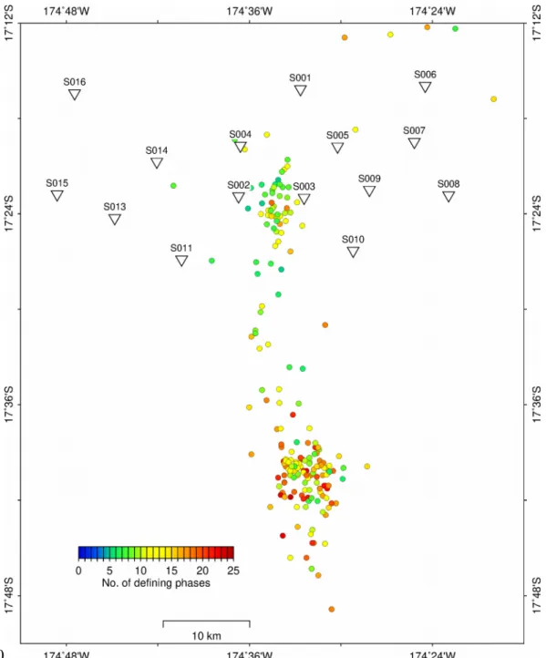
Figure S5. Class A and B events with color code presenting the number of defining phases for individual events. Note that many events in the southern cluster are associated with 20 or more defining phases. On the contrary, most events below the OBS network have only 15 or less defining phases.
21
22
50
51 52
53 54
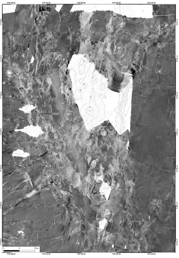
Figure S6. Map showing seafloor backscatter intensity acquired with the Kongsberg EM 122 multibeam echosounder during RV Sonne cruise SO267 (Hannington et al., 2019). Brighter colors represent higher backscatter intensity, darker colors represent lower backscatter intensity. Depths 25
26
55
56 57
58 59
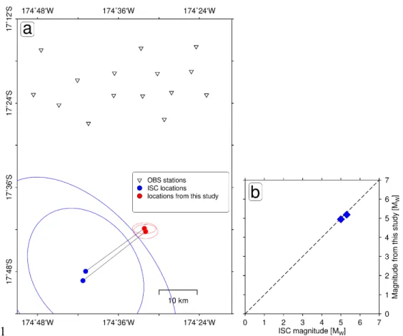
Figure S7. Comparison of the locations (panel a) and moment magnitudes (panel b) for two earthquakes included in our catalog as well as in the bulletin of the International Seismological Center (ISC; www.isc.ac.uk). The origin times of the events in the ISC bulletin deviate less than 0.5 seconds from our catalog and the epicenters coincide reasonably well, re-assuring that these events are actually identical with the ones in our catalog. Blue and red solid lines in panel a show epicenter location error ellipses.
29
30
61
62 63
64 65
66
67 68
Table S1. Settings of the STA/LTA trigger used for the detection of events in the continuous waveform data. STA=short-term-avera, LTA=long-term- average, TH=trigger threshold, Tbefore=length of waveform section extracted before the trigger, Tafter=length of waveform section extracted after the trigger, NETmin=minmum number of station in the network required to define a trigger.
STA [s] LTA [s] TH Tbefore [s] Tafter [s] NETmin
10 110 9 20 160 4
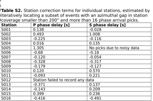
Table S2. Station correction terms for individual stations, estimated by iteratively locating a subset of events with an azimuthal gap in station coverage smaller than 200° and more than 16 phase arrival picks.
Station P phase delay [s] S phase delay [s]
S001 0.138 -0.028
S002 0.493 1.008
S003 -0.225 -0.116
S004 0.016 0.135
S005 1.305 No picks due to noisy data
S006 -0.68 -0.18
S007 -0.120 -0.054
S008 -0.328 -0.317
S009 -0.179 -0.127
S010 0.120 0.570
S011 -0.093 0.221
S012 Station failed to record any data
S013 -0.371 0.137
S014 -0.143 0.209
S015 0.399 0.236
S016 -0.416 -0.491
Table S3. Comparison of different 1D velocity models. The “average Vp- model” represents the one used for locating the entire catalog and is plotted as red line in Figure S1. The “slow Vp-model” represent the “average Vp- model” minus standard deviation of Vp. The “fast Vp-model” represents the
“average Vp-model” plus standard deviation of Vp. Note, the range of standard deviation of Vp is plotted as gray shading in Figure S1. For this comparison, we only used events that have an azimuthal gap in station coverage smaller than 200 degrees and include at least one S-phase pick.
Number of located events
Mean RMS
misfit [s] Mean length of the semi-major axis of
confidence ellipsoid [km]
Mean length of the semi-minor axis of
confidence ellipsoid [km]
Fast Vp-model 58 0.187 4.196 2.250
Average Vp- model
58 0.186 3.861 2.222
Slow Vp-model 58 0.187 3.943 2.241
33