A Generalized ARFIMA Process with Markov-Switching Fractional Differencing Parameter

(1)

SFB 649 Discussion Paper 2007-022

A Generalized ARFIMA Process with

Markov-Switching Fractional Differencing

Parameter

Wen-Jen Tsay*

Wolfgang Härdle**

* Academia Sinica, Taiwan

** Humboldt-Universität zu Berlin, Germany

This research was supported by the Deutsche

Forschungsgemeinschaft through the SFB 649 "Economic Risk".

http://sfb649.wiwi.hu-berlin.de ISSN 1860-5664

SFB 649, Humboldt-Universität zu Berlin Spandauer Straße 1, D-10178 Berlin

S FB

6 4 9

E C O N O M I C

R I S K

B E R L I N

(2)

A Generalized ARFIMA Process with Markov-Switching Fractional Differencing

Parameter

Wen-Jen Tsay

¹

and Wolfgang Karl H¨ardle

² ^∗

April 24, 2007

1 The Institute of Economics, Academia Sinica, Taiwan

2 CASE – Center for Applied Statistics and Economics Humboldt-Universit¨at zu Berlin,

Spandauer Straße 1, 10178 Berlin, Germany Abstract

We propose a general class of Markov-switching-ARFIMA processes in order to combine strands of long memory and Markov-switching literature. Although the coverage of this class of models is broad, we show that these models can be easily estimated with the DLV algorithm proposed. This algorithm combines the Durbin-Levinson and Viterbi procedures. A Monte Carlo experiment reveals that the finite sample performance of the proposed algorithm for a simple mixture model of Markov-switching mean and ARFIMA(1, d,1) process is satisfactory. We apply the Markov-switching-ARFIMA models to the U.S. real interest rates, the Nile river level, and the U.S. unemployment rates, respectively. The results are all highly consistent with the conjectures made or empirical results found in the literature. Particularly, we confirm the conjecture in Be- ran and Terrin (1996) that the observations 1 to about 100 of the Nile river data seem to be more independent than the subsequent observations, and the value of differencing parameter is lower for the first 100 observations than for the subsequent data.

Key words: Markov chain; ARFIMA process; Viterbi algorithm; Long memory

JEL classification: C14, C22, C32, C52, C53, G12

∗This research was supported by the Deutsche Forschungsgemeinschaft through the SFB 649 ‘Economic Risk’. Correspondence to Wen-Jen Tsay. The Institute of Economics, Academia Sinica, Taipei, Taiwan, R.O.C. Tel: (886-2) 2782-2791 ext. 296. Fax: (886-2) 2785-3946. E-Mail: wtsay@ieas.econ.sinica.edu.tw

(3)

1 Introduction

It is well known that many time series data exhibit long memory, or long-range dependence, including the Nile river level, ex postreal interest rate, forward premium, and the dynamics of aggregate partisanship and macroideology. Among the many other examples that Beran (1994) gives the Nile river data has been known for its long memory behavior since an- cient times, and this is one of the time series that led to the discovery of the Hurst effect (Hurst, 1951) and motivated Mandelbrot and his co-workers (Mandelbrot and van Ness, 1968;

Mandelbrot and Wallis, 1969) to introduce fractional Gaussian noise to model long memory phenomenon.

Long range dependence also has been observed in financial data. As demonstrated by Ding et al. (1993), de Lima and Crato (1993) and Bollerslev and Mikkelsen (1996) that the volatility of most financial time series exhibits strong persistency and can be well described as a long memory process. Evidence of financial market volatility’s strong persistency inspired Breidt et al. (1998) to propose a class of long memory stochastic volatility (LMSV) models.

Deo et al. (2006) also show that the LMSV model is useful for forecasting realized volatility (RV) which is an important quantity in finance.

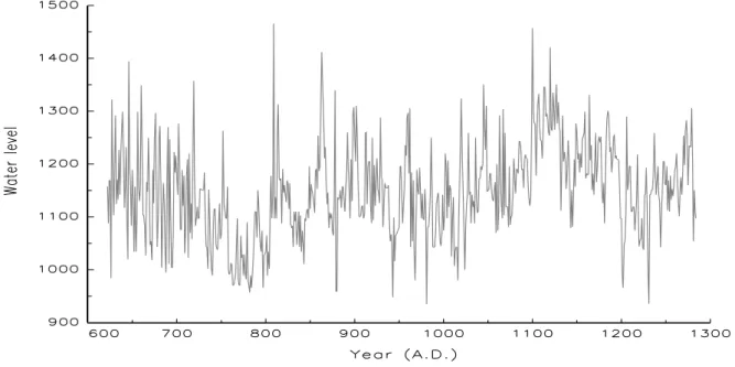
Figure 1 displays the yearly Nile river minima based on measurements at the Roda gauge near Cairo during the years 622-1284. Beran (1994, p.33) documents that “When one only looks at short time periods, then there seem to be cycles or local trend. However, looking at the whole series, there is no apparent persisting cycle.” The changing pattern of the Nile river data leads Bhattacharya et al. (1983) to argue that the so-called Hurst effect can also be explained as if the observations are composed as the sum of a weakly dependent stationary process and a deterministic function. As a consequence it is important to distinguish between a long memory time series and a weakly dependent time series with change-points in the mean. This question has been intensively considered in the literature, including K¨unsch (1986) and Heyde and Dai (1996). Berkes et al. (2006) presents an overview about this strand of literature. Similarly, Diebold and Inoue (2001) shows that long memory also may be easily confused with a Markov-switching mean. Thus, most of the existing literature considers long memory as a competing modeling framework against the structural change and Markov-switching models.

The Nile river level time series is far more complicated than a pure long memory or

(4)

Figure 1: Yearly Nile river minima based on measurements at the Roda gauge near Cairo.

a weakly dependent time series with change-points in the mean to describe. Beran and Terrin (BT) (1996) suggest therefore that the Hurst parameter characterizing the yearly Nile river might change over time. When estimating the Nile river data with the autoregressive fractionally-integrated moving-average (ARFIMA) or I(d) process introduced by Granger (1980), Granger and Joyeux (1980) and Hosking (1981), Beran and Terrin (1996, p.629) show that the data can be well fitted with an ARFIMA(0, d,0) model with d = 0.4, where the fractional differencing parameter d of ARFIMA process acts like the Hurst parameter H of fractional Gaussian noise in characterizing the hyperbolic decay of the autocovariance function of a long memory process. BT further claim that the observations 1 to about 100 seem to be more independent than the subsequent observations, and the value of the fractional differencing parameter might be lower for the first 100 observations than for the subsequent data. If this claim is right, then there should be a structural change in the long range persistence of the Nile river data around the year 720, and the Nile river data neither can be described with a pure long memory nor a weakly dependent time series with change-points in the mean.

The possible change of the differencing parameter stimulate BT to propose a statistic for testing the stability of the fractional differencing parameter. This testing statistic has been further discussed and extended in Horv´ath and Shao (1999) and Horv´ath (2001). However,

(5)

their methods can not identify the change points of the fractional differencing parameter.

A Bayesian random persistent-shift (RPS) method for detecting structural change in the differencing parameter and the process level has been considered in Ray and Tsay (2002).

Nevertheless, the RPS method is not built on the Markov-switching framework, thus may not fully characterize the cycling behavior of the data series, i.e., “seven years of great abundance”

and “seven years of famine” — the Joseph effect named by Mandelbrot and van Ness (1968) and Mandelbrot and Wallis (1969).

The above considerations lead us to combine the long memory and Markov-switching literature into a unified framework. We introduce a Markov-switching-ARFIMA (MS-ARFIMA) process by extending the hidden Markov model. Given that the hidden Markov model has become extremely popular in speech recognition as shown in Juang and Rabiner (1991) and Qian and Titterington (1991), and in econometrics, finance, genetics, and neurophysiology as outlined in Robert et al. (2000), the MS-ARFIMA model provides a flexible modeling framework for many applications to these fields. Moreover, the research conducted in this paper also solve the puzzle raised by Diebold and Inoue (2001) by estimating the differencing parameter allowing for the parameters of interest are Markov-switching.

The remaining parts of this paper are arranged as follows: Section 2 presents the MS- ARFIMA process and the algorithms for estimating the parameters of interest. In Section 3 we consider the finite sample performance of the proposed algorithm under the simple mixture of a Markov-switching mean and an ARFIMA(1, d,1) process. We then apply the proposed methodology to the U.S. real interest rates, the Nile river data, and the U.S. unemployment rates in Section 4. Section 5 provides a conclusion.

2 Models and Main Results

The objective of this paper is to propose a general class of Markov-switching-ARFIMA processes in order to combine strands of long memory and Markov-switching literature. This class of models offers a rich dynamic mixture of a Markov chain and anI(d) process.

Let {s_t}^T_t=1 be the latent sample path of an N-state Markov chain. At each time s_t can

(6)

assume only an integer value of 1,2,· · ·, N, and its transition probability matrix is

P ≡







p11 p21 · · · p_N1

p12 p22 · · · p_N2

... ... ... ...

p1N p2N · · · p_{N N}







,

wherep_ij =P(st =j |s_t−1 =i) and ^P^N_j=1p_ij = 1 for all i.

An I(d) process,x_t, is defined as:

(1−L)^dx_t =h_t,

whereLis the lag operator (Lkt =k_t−1) andh_t is a short memory process. Whend >0, the I(d) process is often called the long memory process, because its autocovariance function is not summable so as to capture the long range dependence of a time series. In addition, the I(d) process is nonstationary when d≥ ¹₂, otherwise, it is covariance stationary.

Combining the defining feature of a Markov chain and that of anI(d) process, we propose the following MS-ARFIMA(p, d, q) process:

w_t=µ_stI{t ≥1}+ (1−L)^−d^stσ_stz_tI{t≥1}=µ_stI{t≥1}+y_st, (1) whereI{.}is the indicator function andz_tis stationary process with mean zero and bounded positive spectral density f_u(λ) ∼ G0 as λ → 0 at each possible regime, thus including stationary and invertible ARMA process as its special case. The most distinguished feature of the process is that the fractional differencing parameterd_st well known in the long memory literature is allowed to be a Markov chain satisfying the following Assumption A:

Assumption A.s_t is independent of z_τ for all t and τ.

The model in (1) subsumes many interesting models in the literature. When N = 1, w_t reduces to the specification in (7) of Shimotsu and Phillips (2005):

w_t =µ0+ (1−L)^−d⁰σ0z_tI{t≥1} (2) which also can be represented as:

w_t=µ0+

t−1

X

k=0

(d0)k

k σ0z_t−k, (3)

(7)

where

(d0)k= Γ(d0+k)

Γ(d0) = (d0)(d0+ 1). . .(d0+k−1) (4) is Pochhammer’s symbol for the forward factorial and Γ(.) is the gamma function. More- over, under the model in (1) and d_s_t = 0, w_t still includes the Markov-switching AR model considered in Hamilton (1989) as one of its special cases. We will show that the estimation of the model in (1) can be easily implemented with the algorithm proposed in this paper, even though the parameter estimation from a noisy version of realizations of Markov models is extremely difficult in all but very simple examples as well documented in Qian and Titterington (1991).

Let the total sample size be T, and denote Wt ≡ (w1, w2,· · ·, w_t)^⊤ the column vector containing the observations from time 1 to time t, while St = (s1, s2,· · ·, s_t)^⊤ represents the corresponding states, and Yt = (y1, y2,· · ·, y_t)^⊤ in (1) is similarly defined. The column vector α = (µ1, . . . , µ_N, σ1, . . . , σ_N, φ11, . . . , φ1p, φ21, . . . , φ_{N p}, d1, . . . , d_N, θ11,· · ·, θ_{N q})^⊤ and p_ij (transition probabilities) consist of the parameters characterizing the conditional density function (cdf) of w_t. After stacking the parameter vector α and the transition probabilities p_ij into one column vector ξ, we can represent the cdf of w_t as f(wt| St,Wt−1;ξ), clearly showing that the cdf of w_t depends on the entire past routes of states (in general). Indeed, there are N^T possible paths of states running throughout the observations WT.

To illustrate the proposed algorithm for the model in (1), we first consider the simplest case wherew_t in (1) is generated as:

w_t=µ_s_tI{t≥1}+ (1−L)^−d⁰σ0ε_tI{t≥1}=µ_s_tI{t≥1}+y_t, (5) whered < ¹₂ and ε_t is a zero mean normally, independently and identically distributed white noise (i.i.d.) with E(ε²_t) = 1. That is, w_t in (5) is a special type of MS-ARFIMA(0, d,0) process whose differencing parameter is fixed across different regimes. Under Assumption A andε_t ∼N(0,1) i.i.d. process, the likelihood function ofWT,L(ST,WT;ξ) hereafter, for the hidden Markov model in (5) equals

L(ST,WT;ξ) = (2π)^{−T /}²|Λ|⁻¹^/²exp

−1

2Y_T^⊤Λ⁻¹YT

YT t=1

Pr(st |s_t−1), (6) where Λ = E(YTY_T^⊤), and Pr(s1 | s0) is evaluated with the unconditional probability that the process will be in regime s1. Given that y_t in (5) is a simple ARFIMA(0, d,0) process,

(8)

we can use the Durbin-Levinson algorithm to derive (2π)^{−T /}²|Λ|⁻¹^/²exp

−1

2Y_T^⊤Λ⁻¹YT

=

YT t=1

(2π)⁻¹^/²v⁻_t−¹1^/²exp

(

−(yt−yb_t)² 2v_t−1

)

, (7)

where yb_t denotes the one-step ahead predictor of y_t with the observation Yt−1 as j ≥ 2, andv_t−1 is the corresponding one-step ahead prediction variance. Deriche and Tewfik (1993) also have employed the Durbin-Levinson algorithm to estimate a univariate ARFIMA(0, d,0) processes without Markov-switching characteristic. Note that as t = 1, yb1 = 0, and v0 =γ0

corresponds to the variance ofy_t. As a result, the likelihood function in (6) can be rewritten as:

L(ST,WT;ξ) =

YT t=1

(2π)⁻¹^/²v_t−⁻¹₁^/²exp

(

−(y_t−yb_t)² 2vt−1

)

Pr(s_t|s_t−1), (8) indicating that the unconditional likelihood function of the mixture model in (5) can be exactly and recursively evaluated provided that we can identify the true path of s_t, S_T^∗.

We do not know in reality the value ofS_T^∗. However, the recursive structure shown in (8) is especially suitable for implementing the Viterbi (1967) algorithm in the digital commu- nication literature to identify the most likely path of states among the N^T possible routes within WT. We thus combine the Durbin-Levinson algorithm and the Viterbi algorithm to suggest a Durbin-Levinson-Viterbi (DLV) algorithm for the model in (5). When compared to the original Viterbi algorithm designed for solving the problem of maximum a posteri- ori probability estimate of the state sequence of a finite-state discrete-time Markov process observed in white noise, the DLV algorithm proposed in this paper is concerned with the hidden Markov process observed in a much more general ARFIMA noise. Since the DLV algorithm can estimate the differencing parameter of a time series allowing for the presence of a Markov-switching mean, the puzzle raised by Diebold and Inoue (2001) that long memory can be easily confused with a Markov-switching mean is thus resolved by using this DLV algorithm.

To locate the most likely path running through the data WT with the idea of Viterbi (1967), we note first that, for each timet, there areN possible states ending at time t, i.e., (st = i), i = 1, . . . , N. For a particular node of these N end points at time t, say (st =j), there exists a corresponding most likely path:

(St−1(st =j), st=j) = (s1(st=j), s2(st=j),· · ·, s_t−1(st=j), st=j), (9)

(9)

which ends at this particular node (st = j). We refer to the path (St−1(st = j), st = j) in (9) as the survivor associated with the node (st = j). Note that, with little loss of clarity, we do not explicitly specify that the path depends on the parameter ξ and the observations Wt in order to simplify the notation. The likelihood function generated from this survivor (St−1(st=j), st =j) and the formula in (8) is recorded asL(St−1(st=j), st =j,Wt;ξ) and is crucial for locating the most likely path running from time 1 to timeT. In short, for each node (st=j) at timet, there exists a most likely path, survivor (St−1(st =j), st=j), and its associated likelihood function L(St−1(s_t =j), s_t = j,Wt;ξ). Most importantly, the number of survivors at each timet is always equal to N.

Given theN survivors at timetand in order to locate the survivor (St(s_t+1 =i), s_t+1 =i) for a particular node (s_t+1 =i) at time t+ 1, among the N segments connecting the node (s_t+i =i) and the N time-t survivors (S_t−1(s_t =j), s_t =j) recorded at time t, we select the one producing the largest likelihood function L(S_t(s_t+1 =i), s_t+1 =i,W_t+1;ξ) among these N possible candidates, and name it as the survivor (St(st+1 =i), st+1 =i) for this particular node (st+1 = i). The computation of the aforementioned likelihoods is simple, because we record the likelihood functions of theN time-t survivors at each time t.

This recursive updating process proceeds from time 1 to time T and results in N time- T survivors (ST−1(sT = i), sT = i) and their associated likelihood function L(ST−1(sT = i), sT = i,WT;ξ), for each i = 1, . . . , N. From these N time-T survivors we select the one producing the largest likelihood function, say L(ST−1(sT = g), sT = g,WT;ξ), as the most likely path running from time 1 to time T. Combining a numerical optimization procedure and this chosen likelihood function L(ST−1(sT = g), sT = g,WT;ξ) generated from the Viterbi algorithm and the Durbin-Levinson algorithm displayed in (7), we can estimate the parametersξ and identify the states ST hidden in the observationsWT.

We now consider another special type of MS-ARFIMA(p, d, q) process:

w_t=µ_s_tI{t ≥1}+y_t=µ_s_tI{t≥1}+ (1−L)^−d⁰σ0z_tI{t≥1}, φ(L)z_t =θ(L)ε_t, (10) where

φ(L) = 1−φ1L−. . .−φ_pL^p, θ(L) = 1 +θ1L+. . .+θ_qL^q, (11) and the roots of the polynomialφ(L) and those ofθ(L) in (11) are all outside the unit circle and share no common roots. The model in (10) is much more general than that in (5), but

(10)

still can be estimated with the preceding Viterbi algorithm after some modifications. Please note that the value of fractional differencing parameter is unchanged across different regimes as that imposed in (5).

Note that the termy_t in (10) can be rearranged as

y_t= (1−L)^−d⁰σ0φ(L)⁻¹θ(L)ε_t, t= 1,2, . . . . (12) We then have

φ(L)yt= (1−L)^−d⁰σ0θ(L)εt=σ0θ(L)(1−L)^−d⁰ε_t=σ0θ(L)ye_t, t= 1,2, . . . , (13) where ye_t = (1−L)^−d⁰ε_t is an ARFIMA(0, d,0) process. Dueker and Serletis (2000) use the same transformation method for estimating an ARFIMA(p, d, q) process. Conditional on a set of φ(L) and θ(L) and a suitable starting value, the conditional likelihood function of y_t in (12) can still be evaluated exactly with the transformed ARFIMA(0, d,0) ye_t in (13) and the Durbin-Levinson algorithm defined in (7). For example, conditional ony0 being equal to 0, we can extract an ARFIMA(0, d,0) process from an ARFIMA(1, d,1) process as follows:

σ0ye_t=y_t−φ1y_t−1−σ0θ1ye_t−1, t= 1, . . . , T. (14) Conditional on a set ofφ(L) and θ(L) and a suitable starting value for the parameter ξ, we can recursively and exactly evaluate the conditional likelihood function of the hidden Markov model using the DLV algorithm proposed previously.

The same idea also applies to the class of MS-ARFIMA(p, d, q) processes in (1) where d can be Markov-switching. However, we cannot use the Durbin-Levinson algorithm when the fractional differencing parameter is allowed to be Markov-switching. Nevertheless, the Viterbi algorithm is still powerful enough to locate the most likely path under this circumstance.

That is, conditional on a suitable starting value for the parameterξ, we employ the recursive structure inherent in Viterbi algorithms to identify the most likely path running through the data set.

3 Monte Carlo Experiment

In this section we consider a Monte Carlo experiment to demonstrate the finite sample performance of the proposed DLV algorithm on a special version of the model in (1):

w_t=µ_stI{t≥1}+ (1−L)^−d⁰σ0(1−φ1L)⁻¹(1 +θ1L)εtI{t≥1}. (15)

(11)

We employ three different values of the fractional differencing parameter:

d0 ={0.2,0.3,0.4}, (16) along with the following parameters:

µ1 = 4, µ2 = 1, φ1 = 0.5, θ1 = 0.5, p11 =p22= 0.95, (17) and σ0 is chosen to ensure that the variance of the ARFIMA(1, d,1) noise in (15) is equal to 1 across different configurations. Note that the positive values of d0 in (16) are chosen to reflect the variations used in the long memory literature.

All the computations are performed with GAUSS. Two hundred replications are conducted for each specification at 3 different sample sizes (T = 100,200,400) usually encountered in the empirical applications. For each sample size T, 200 additional values are generated in order to obtain random starting values. The optimization algorithm used to implement the DLV algorithm is the quasi-Newton algorithm of Broyden, Fletcher, Goldfarb, and Shanno (BFGS) contained in the GAUSS MAXLIK library. The maximum number of iterations for each replication is 100.

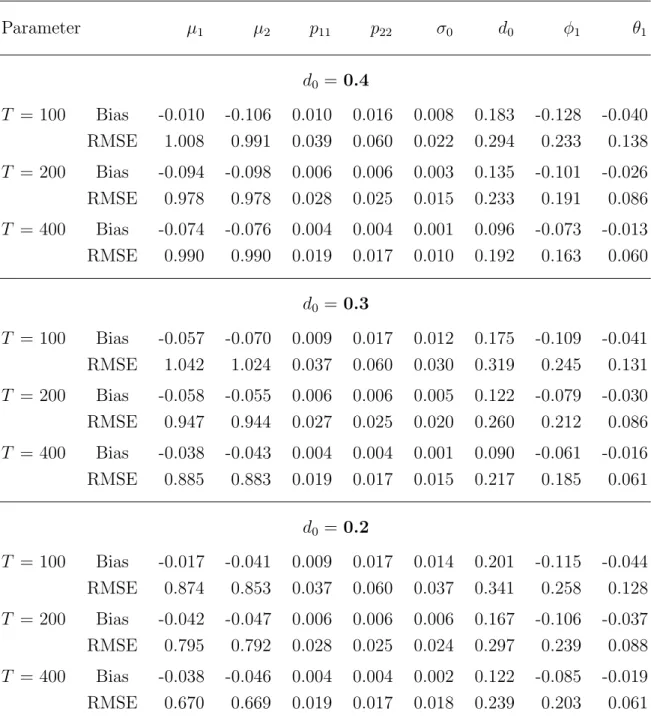
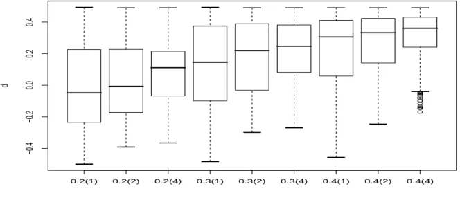
Table 1 contains the simulation results when the true value of parameters are used as the initial values for estimation procedure. The results reveal that the bias performance from the DLV algorithm is satisfactory (especially when the sample size is larger) for all configurations considered. Moreover, the associated root-mean-squared error (RMSE) almost always decreases with the increasing sample size. We find only two cases where the pattern of RMSE change is not what we expect, i.e., when d0 = 0.4, the RMSE of estimating the parameters µ1 and µ2 as T = 400 is found to be a little higher than that of estimating the parameters µ1 and µ2 as T = 200. These two observations demonstrate the ability of the DLV algorithm to deal with the mixture model considered in this section. The performance of DLV algorithm for estimating the fractional differencing parameter is particularly displayed with the box-plots in Figure 2. The above-mentioned observations are clearly borne out in this figure.

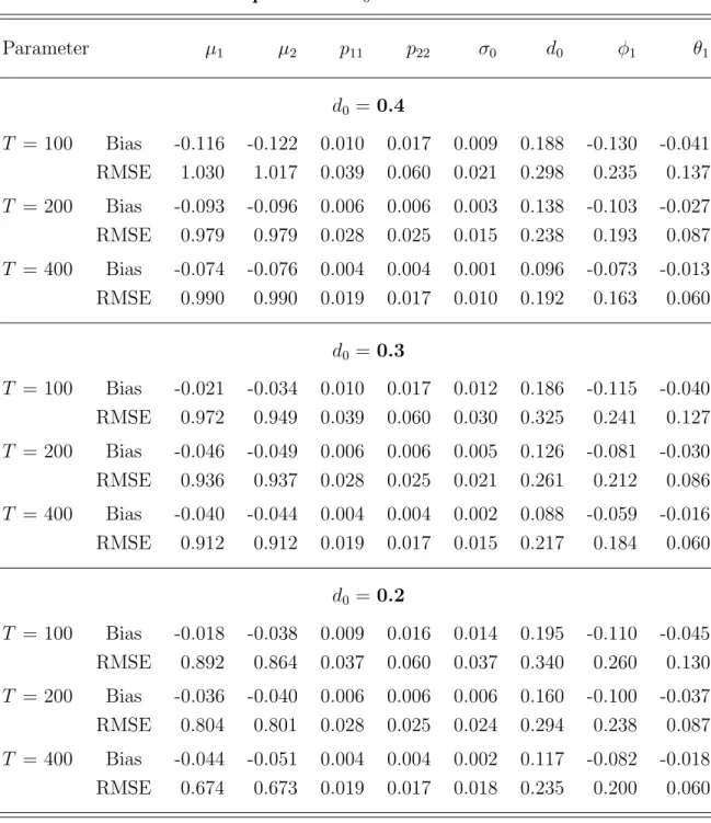
We also check the robustness of the preceding simulation results by changing the choice of initial values for estimation. The simulations in Table 1 are replicated by setting the initial values for parameters at the true values except that of d0 is set at zero. The results

(12)

Table 1. Finite sample performance of the DLV algorithm:

Initial values of parameters are set at the true values of parameters

Parameter µ1 µ2 p11 p22 σ0 d0 φ1 θ1

d0 =0.4

T = 100 Bias -0.010 -0.106 0.010 0.016 0.008 0.183 -0.128 -0.040 RMSE 1.008 0.991 0.039 0.060 0.022 0.294 0.233 0.138 T = 200 Bias -0.094 -0.098 0.006 0.006 0.003 0.135 -0.101 -0.026 RMSE 0.978 0.978 0.028 0.025 0.015 0.233 0.191 0.086 T = 400 Bias -0.074 -0.076 0.004 0.004 0.001 0.096 -0.073 -0.013 RMSE 0.990 0.990 0.019 0.017 0.010 0.192 0.163 0.060

d0 =0.3

d0 =0.2

T = 100 Bias -0.017 -0.041 0.009 0.017 0.014 0.201 -0.115 -0.044 RMSE 0.874 0.853 0.037 0.060 0.037 0.341 0.258 0.128 T = 200 Bias -0.042 -0.047 0.006 0.006 0.006 0.167 -0.106 -0.037 RMSE 0.795 0.792 0.028 0.025 0.024 0.297 0.239 0.088 T = 400 Bias -0.038 -0.046 0.004 0.004 0.002 0.122 -0.085 -0.019 RMSE 0.670 0.669 0.019 0.017 0.018 0.239 0.203 0.061 Notes: Simulations are based on 200 replications. The data is generated from the mixture model defined in (15), (16) and (17). DLV algorithm is the Durbin-Levinson- Viterbi algorithm proposed in this paper. Bias is computed as the true parameter minus the corresponding average estimated values.

(13)

0.2(1) 0.2(2) 0.2(4) 0.3(1) 0.3(2) 0.3(4) 0.4(1) 0.4(2) 0.4(4)

−0.4−0.20.00.20.4

d

Figure 2: Box-plots of the estimateddfrom the model defined in (15), (16) and (17) with 200 realizations.

The initial values of parameters are set at the true values of parameters. The valuef(g) denotes the model specification whered=f and T = 100×g.

contained Table 2 and Figure 3 indicate that the finite sample performance of our procedure is not sensitive to the initial values used for estimation.

4 Empirical Applications

The methodology developed in this paper is motivated by the dynamic pattern of long memory behavior. Evidence has been given by many methods for such a changing covariance behavior of the Nile river. The applications of the proposed MS-ARFIMA model to actual data are far reaching. For that reason, we consider three data set. The first one is the U.S. real interest rates, the second one is the Nile river data, and the third one is the U.S.

unemployment rates.

4.1 Example with real interest rates

In this subsection we first consider the U.S. ex post monthly real interest rate constructed from monthly inflation and Treasury bill rates from January 1953 to December 1990 in Mishkin (1990). The reason we use the original dataset of Mishkin (1990) is to employ it as a benchmark for a clear comparison between the results from the MS-ARFIMA model and

(14)

Table 2. Finite sample performance of the DLV algorithm:

Initial values of parameters are set at the true values of parameters except that of d0 is set at zero

Parameter µ1 µ2 p11 p22 σ0 d0 φ1 θ1

d0 =0.4

d0 =0.3

d0 =0.2

T = 100 Bias -0.018 -0.038 0.009 0.016 0.014 0.195 -0.110 -0.045 RMSE 0.892 0.864 0.037 0.060 0.037 0.340 0.260 0.130 T = 200 Bias -0.036 -0.040 0.006 0.006 0.006 0.160 -0.100 -0.037 RMSE 0.804 0.801 0.028 0.025 0.024 0.294 0.238 0.087 T = 400 Bias -0.044 -0.051 0.004 0.004 0.002 0.117 -0.082 -0.018 RMSE 0.674 0.673 0.019 0.017 0.018 0.235 0.200 0.060 Notes: Simulations are based on 200 replications. The data is generated from the mixture model defined in (15), (16) and (17). DLV algorithm is the Durbin-Levinson- Viterbi algorithm proposed in this paper. Bias is computed as the true parameter minus the corresponding average estimated values.

(15)

0.2(1) 0.2(2) 0.2(4) 0.3(1) 0.3(2) 0.3(4) 0.4(1) 0.4(2) 0.4(4)

−0.4−0.20.00.20.4

d

Figure 3: Box-plots of the estimateddfrom the model defined in (15), (16) and (17) with 200 realizations.

The initial values of parameters are set at the true values except that of d⁰ is set at zero. The valuef(g) denotes the model specification whered=f andT = 100×g.

those generated from the methodology employed in earlier papers.

The main feature of the real interest rate is that the whole dataset can be split into three subperiods, January 1953-October 1979, November 1979-October 1982, and November 1982-December 1990, because the operating procedure of the monetary authority changed in October 1979 and October 1982 as argued in Mishkin (1990). Another interesting feature of the real interest rate is that the data of these three subperiods can be well described with the ARFIMA models as shown in Tsay (2000). The simultaneous presence of structural break and long memory within the real interest rate allows itself to be an ideal subject to be investigated with the MS-ARFIMA model.

Allowing the break points to be endogenously determined, Table 3 contains the parameter estimates from the following mixture model with a 2-state Markov chain and an ARFIMA(1, d,1) noise:

w_t=µ_stI{t ≥1}+ (1−L)^−d⁰σ0z_tI{t ≥1}, (1−φ1L)z_t= (1 +θ1L)ε_t, (18) whereφ1orθ1is assumed to be zero depending on the noise specification. Following Hamilton (1989), asymptotic standard errors are calculated numerically.

Table 3 shows that the estimates of µ1, µ2, p11, p22, σ0, and d0 from the DLV algorithm

(16)

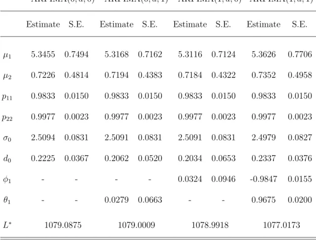
Table 3. Estimates of Parameters Based on Data for U.S. Monthly Real Interest Rate and the DLV Algorithm

ARFIMA(0, d,0) ARFIMA(0, d,1) ARFIMA(1, d,0) ARFIMA(1, d,1) Estimate S.E. Estimate S.E. Estimate S.E. Estimate S.E.

µ1 5.3455 0.7494 5.3168 0.7162 5.3116 0.7124 5.3626 0.7706 µ2 0.7226 0.4814 0.7194 0.4383 0.7184 0.4322 0.7352 0.4958 p11 0.9833 0.0150 0.9833 0.0150 0.9833 0.0150 0.9833 0.0150 p22 0.9977 0.0023 0.9977 0.0023 0.9977 0.0023 0.9977 0.0023 σ0 2.5094 0.0831 2.5091 0.0831 2.5091 0.0831 2.4979 0.0827 d0 0.2225 0.0367 0.2062 0.0520 0.2034 0.0653 0.2337 0.0376

φ1 - - - - 0.0324 0.0946 -0.9847 0.0155

θ1 - - 0.0279 0.0663 - - 0.9675 0.0200

L^∗ 1079.0875 1079.0009 1078.9918 1077.0173

Notes: The results are based on the MS-ARFIMA model defined in (18). S.E. stands for the standard error of the estimate. L^∗represents the negative of the log-likelihood function of the switching model. DLV algorithm is the Durbin-Levinson-Viterbi algorithm proposed in this paper.

(17)

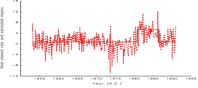
Figure 4: US monthly ex post real interest rates, January 1953-December 1990. Solid line denotes the path of estimated switching means from the specification ARFIMA(0, d,0) in Table 3, while dotted line denotes the observed monthly ex post real interest rates.

are quite robust across all 4 different configurations. More importantly, two identical break points are identified with these four models, thus divide the whole data into three subperiods as suggested in Mishkin (1990). The endogenous break points identified are November 1980 and May 1986, respectively.

Figure 4 displays the U.S. monthly ex post real interest rates and the path of estimated switching means generated from the DLV algorithm. Without loss of generality, only the path of the estimated switching means from the specification ARFIMA(0, d,0) in Table 3 is reported. Figure 4 shows that the model in (18) provides a satisfactory fitting of the U.S.

monthly real interest rates. Although the endogenously identified break points are later than the well-known monetary operating procedure change points (October 1979 and October 1982), this finding is quite reasonable, because it takes some time for the ex post real interest rate to adjust its path after new information arrives. This argument is buttressed with the findings in Figure 4 that the endogenously identified break points are more closely connected to the observed path of the U.S. monthly ex post real interest rates than the monetary operating procedure change points are.

Table 3 also shows that a long memory phenomenon is found in the real interest rate as has been documented in Tsay (2000). Nevertheless, the estimate of the fractional differencing parameter in Table 3 is much lower than that of 0.666 in Table 3 of Tsay (2000) where the

(18)

change points are exogenenously determined, and it is more in line with the estimates of 0.204, 0.275, and 0.193 from the individual subperiod data presented in Table 3 of Tsay (2000). This implies that the persistence of long memory in the real interest rate is much more mitigated, once we take the potentially switching mean of the data into account, thus confirming the arguments of Diebold and Inoue (2001) that the presence of Markov-switching level might increase the persistence of the data under investigation.

4.2 Example with Nile river data

In this subsection we apply the Viterbi algorithm to the Nile river data with the following model:

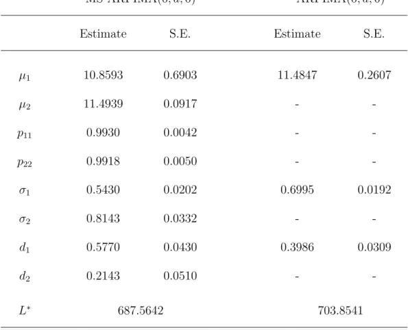
w_t=µ_s_tI{t ≥1}+ (1−L)^−d^stσ_s_tε_tI{t≥1}, (19) where N is assumed to be 2. For the purpose of comparison, we estimate a fixed regime ARFIMA(0, d,0) model for the Nile river data, i.e., N = 1 is imposed on this model. The estimated value ofdfrom such a fixed regime ARFIMA(0, d,0) model is 0.3986 and is almost identical to the finding in Beran and Terrin (1996).

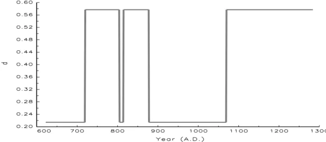
When estimating the model in (19) with the Viterbi algorithm, we find that the value of the differencing parameter in Table 4 is 0.5770 (nonstationary) for one state, and is 0.2143 (stationary) for the other one. In addition, we identify 5 transitions within the Nile river data in the year 720, 805, 815, 878, and 1070. The estimated path of d_st from the MS- ARFIMA(0, d,0) model in Table 4 is graphed in Figure 5.

Most impressively, the first transition data occurs in the year of 720, and the associated estimated value ofd_s_t within the period 622 to 719 is 0.2143 which is lower than the 0.5770 observed in the other regime. These two findings correspond closely to the conjectures in Beran and Terrin (1996) that the observations 1 to about 100 seem to be more independent than the subsequent observations and the value of differencing parameter might be lower for the first 100 observations than for the subsequent data.

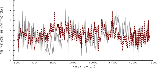
In Figures 6 and 7 we present the observations and the fitted values generated from the estimated parameters displayed in Table 4. It is clear that the fitted value from the MS-ARFIMA(0, d,0) model is much closer to the real data than that generated from the model whose differencing parameter is not Markov switching. Combining the findings of the likelihood values in Table 4, we find that the MS-ARFIMA(0, d,0) model is a promising

(19)

Table 4. Estimates of MS-ARFIMA(0, d,0) Model based on the Nile River Data

MS-ARFIMA(0, d,0) ARFIMA(0, d,0)

Estimate S.E. Estimate S.E.

µ1 10.8593 0.6903 11.4847 0.2607

µ2 11.4939 0.0917 - -

p11 0.9930 0.0042 - -

p22 0.9918 0.0050 - -

σ1 0.5430 0.0202 0.6995 0.0192

σ2 0.8143 0.0332 - -

d1 0.5770 0.0430 0.3986 0.0309

d2 0.2143 0.0510 - -

L^∗ 687.5642 703.8541

Notes: The MS-ARFIMA(0, d,0) model is defined in (19). S.E. stands for the standard error of the estimate based on numerical derivative. L^∗ represents the negative of the log-likelihood function of the estimated model.

(20)

Figure 5: Estimateddst from the MS-ARFIMA(0, d,0) model in Table 4.

Figure 6: Solid line denotes the Nile river water level divided by 100, while dotted line denotes the corresponding fitted values from the MS-ARFIMA(0, d,0) model in Table 4.

(21)

Figure 7: Solid line denotes the Nile river water level divided by 100, while dotted line denotes the corresponding fitted values from the ARFIMA(0, d,0) model in Table 4.

alternative to describe the Nile river data.

4.3 Example with unemployment rates

In this subsection we apply the Viterbi algorithm to the U.S. quarterly unemployment rates rates from 1948 to 2006. This data is based on the monthly unemployment rates contained inBureau of Labour Statisticsas those employed in van Dijk et al. (2002) for estimating a fractionally integrated smooth transition autoregressive (FI-STAR) model. However, van Dijk et al (2002) employ the original monthly unemployment rates ranging from July 1986 to December 1999, while we use all the data contained in Bureau of Labour Statistics, but focusing on the quarterly frequency usually considered in the business cycle related studies.

As clearly argued in van Dijk et al. (2002) and shown in Figure 8, there are two important empirical features of U.S. unemployment rates, i.e., the shocks to the series is quite persistent and the series seem to rise faster during recessions than it falls during expansions. van Dijk et al. (2002) find that the estimateddis 0.43 from a FI-STAR model presented in their Table 1.

This implies that a time series model describing long memory and nonlinearity simultaneously may be useful for modeling U.S. unemployment rates and many other applications.

The aforementioned two features contained in U.S. unemployment also provide another good opportunity to test the applicability of the MS-ARFIMA model. As a consequence we estimate the U.S. quarterly unemployment rates with the following MS-ARFIMA(p, d,0)

(22)

Figure 8: U.S. quarterly seasonally adjusted unemployment rates, 1948-2006.

model:

w_t =µ_stI{t≥1}+ (1−L)^−d^stσ_stφ(B)⁻¹ε_tI{t≥ 1}, (20) where N is assumed to be 2, and p = {3,4}. The choice of p = 4 is adopted by following the model specification in (30) of van Dijk et al (2002), while p = 3 is chosen to check the robustness of the estimation results from the specificationp= 4. The major objective of this subsection is to investigate whether the long memory observed in van Dijk et al. (2002) can also be retained from the MS-ARFIMA methodology.

When estimating the model in (20) with the Viterbi algorithm, we find that the values of the estimated fractional differencing parameter from both MS-ARFIMA(3, d,0) and MS- ARFIMA(4, d,0) models in Table 5 are very close to that found in van Dijk et al. (2002), thus confirming that long memory phenomenon seems to be present in the U.S. unemployment rates. For clarity of exposition, the estimated path of d_st from the MS-ARFIMA(3, d,0) model and that ofd_st from the MS-ARFIMA(4, d,0) one are graphed in Figure 9 and Figure 10, respectively. These figures clearly show that d_st are around 0.4-0.5 for both regimes estimated in each MS-ARFIMA(p, d,0) model in Table 5.

We also check to what extent the fitted values generated from the models in Table 5 can capture the feature of U.S. unemployment rates. This task is not taken in van Dijk et al.

(2002) when estimating their FI-STAR model for the U.S. monthly unemployment rates. It is interesting to find in Figure 11 and Figure 12 that the MS-ARFIMA(p, d,0) model in (20)

(23)

Table 5. Estimates of MS-ARFIMA(p, d,0) Model based on the U.S.

quarterly unemployment rates

MS-ARFIMA(3, d,0) MS-ARFIMA(4, d,0)

Estimate S.E. Estimate S.E.

µ1 3.8080 0.1552 3.4572 0.3711

µ2 5.1358 0.4403 3.8254 0.3334

p11 0.9939 0.0067 0.9877 0.0093

p22 0.9896 0.0083 0.9867 0.0101

σ1 0.1973 0.0135 0.1535 0.0101

σ2 0.3380 0.0206 0.3921 0.0274

d1 0.4919 0.1215 0.4429 0.0987

d2 0.4143 0.1337 0.4342 0.1058

φ1 1.2570 0.1415 1.1325 0.1215

φ2 -0.3822 0.1510 -0.2301 0.1239

φ3 -0.0666 0.0788 -0.0141 0.1053

φ4 - - -0.0495 0.0712

L^∗ 36.1377 14.7662

Notes: The results are based on the MS-ARFIMA(p, d,0) model defined in (20).

S.E. stands for the standard error of the estimate based on numerical derivative.

L^∗ represents the negative of the log-likelihood function of the estimated model.

(24)

(25)

Figure 11: Solid line denotes the U.S. quarterly seasonally adjusted unemployment rates (1948-2006), while dotted line denotes the corresponding fitted values from the MS-ARFIMA(3, d,0) model in Table 5.

provides a reasonable fit to the data, even though we do not include some seasonal control variables, like seasonal difference operator, as van Dijk et al. (2002) have done for their empirical studies.

5 Conclusions

A general class of MS-ARFIMA processes is suggested to combine long memory and Markov- switching models into one unified framework. The coverage of this class of MS-ARFIMA models is far-reaching, but we show that they still can be easily estimated with the original Viterbi algorithm or the DLV algorithm proposed in this paper. In addition, the simulation reveals that the finite sample performance of the DLV algorithm for a simple mixture model of Markov-switching mean and ARFIMA(1, d,1) process is satisfactory. When applying the MS-ARFIMA models to the U.S. real interest rates, the Nile river level, and the U.S. unemployment rates, the estimation results are both highly compatible with the conjectures made in the literature. Accordingly, the MS-ARFIMA model considered in this paper not only can be used for solving the puzzle raised by Diebold and Inoue (2001), but can also find many potential applications in several scientific research fields.

(26)

Figure 12: Solid line denotes the U.S. quarterly seasonally adjusted unemployment rates (1948-2006), while dotted line denotes the corresponding fitted values from the MS-ARFIMA(4, d,0) model in Table 5.

References

Beran, J. (1994),Statistics for Long-Memory Processes. New York: Chapman and Hall.

Beran, J. and Terrin, N. (1996), “Testing for a Change of the Long-Memory Parameter”, Biometrika, 83, 627-638.

Berkes, I., Horv´ath, L., Kokoszka, P. and Shao, Q.M. (2006), “On Discriminating between Long-Range Dependence and Changes in Mean”,The Annals of Statistics, 34, 1140-1165.

Bhattacharya, R.N., Gupta, V.K. and Waymire, E. (1983), “The Hurst Effect under Trends”, Journal of Applied Probability, 20, 649-662.

Bollerslev, T. and Mikkelsen, H.O.A. (1996), “Modeling and Pricing Long-Memory in Stock Market Volatility”, Journal of Econometrics, 73, 151-184.

Breidt, F.J., Crato, N. and de Lima, P. (1998), “The Detection and Estimation of Long Memory in Stochastic Volatility”,Journal of Econometrics, 83, 325-348.

de Lima, P. and Crato, N. (1993), “ Long-Range Dependence in the Conditional Variance of Stock Returns”, Proceedings of the Business and Economic Statistics Section, August 1993 Joint Statistical Meetings, San Francisco.

(27)

Deo, R., Hurvich, C. and Lu, Y. (2006), “Forecasting Realized Volatility Using a Long- Memory Stochastic Volatility Model: Estimation, Prediction and Seasonal Adjustment”, Journal of Econometrics 131, 29-58.

Deriche, J.A. and Tewfik, A.H. (1993), “Maximum Likelihood Estimation of the Parame- ters of Discrete Fractionally Differenced Gaussian Noise Process,”IEEE Transactions on Signal Processing, 41, 2977-2989.

Diebold, F.X. and Inoue, A. (2001), “Long Memory and Regime Switching”, Journal of Econometrics, 105, 131-159.

Ding, Z., Granger, C.W.J. and Engle, R.F. (1993), “A Long Memory Property of Stock Market Returns and a New Model”, Journal of Empirical Finance, 1, 83-106.

Dueker, M. and Serletis, A. (2000), “Do Real Exchange Rates Have Autoregressive Unit Roots? A Test under the Alternative of Long Memory and Breaks”, Working Paper 2000-016A, Federal Reserve Bank of St. Louis.

Granger, C.W.J. (1980), “Long Memory Relationships and the Aggregation of Dynamic Models”, Journal of Econometrics, 14, 227-238.

Granger, C.W.J. and Joyeux, R. (1980), “An Introduction to Long-Memory Time Series Models and Fractional Differencing”, Journal of Time Series Analysis, 1, 15-29.

Hamilton, J.D. (1989), “A New Approach to the Economic Analysis of Nonstationary Time Series and the Business Cycle”, Econometrica, 57, 357-384.

Heyde, C.C. and Dai, W. (1996), “On the Robustness to Small Trends of Estimation based on the Smoothed Periodogram”,Journal of Time Series Analysis, 17, 141-150.

Horv´ath, L. (2001), “Change-Point Detection in Long-Memory Processes. Journal of Multi- variate Analysis, 78, 218-234.

Horv´ath, L. and Shao, Q.M. (1999), “Limit Theorems for the Union-Intersection Test”, Journal of Statistical Planning and Inference, 44, 133-148.

Hosking, J.R.M. (1981), “Fractional Differencing”,Biometrika, 68, 165-176.

(28)

Hurst, H.E. (1951), “Long-Term Storage Capacity of Reservoirs”,Transactions of the Amer- ican Society of Civil Engineers, 116, 770-799.

Juang, B.H. and Rabiner, L.R. (1991), “Hidden Marker Models for Speech Recognition”, Technometrics, 33, 251-272.

K¨unsch, H. (1986), “Discrimination between Monotonic Trends and Long-Range Depen- dence”, Journal of Applied Probability, 23, 1025-1030.

Mandelbrot, B.B. and van Ness, J.W. (1968), “Fractional Brownian Motions, Fractional Noises and Applications”, SIAM Review, 10, 422-437.

Mandelbrot, B.B. and Wallis, J.R. (1969), “Some Long-Run Properties of Geophysical Records”, Water Resources Research, 5, 321-340.

Mishkin, F.S. (1990), “What does the Term Structure of Interest Rate Tell Us about Future Inflation? Journal of Monetary Economics, 25, 77-95.

Qian, W. and Titterington, D.M. (1991), “Estimation of Parameters in Hidden Markov Models”, Philosophical Transactions: Physical Sciences and Engineering, 337, 407-428.

Ray, B.K. and Tsay, R.S. (2002), “Bayesian Methods for Change-Point Detection in Long- Range Dependent Process”, Journal of Time Series Analysis, 23, 687-705.

Robert, C.P., Ryd´en, R. and Titterington, D.M. (2000), “Bayesian Inference in Hidden Markov Models through the Reversible Jump Markov Chain Monte Carlo Method”,Jour- nal of the Royal Statistical Society B, 62, 57-75.

Shimotsu, K. and Phillips, P.C.B. (2005), “Exact Local Whittle Estimation of Fractional Integration”,The Annals of Statistics, 33, 1890-1933.

Tsay, W.J. (2000), “Long Memory Story of the Real Interest Rate”, Economic Letters, 67, 325-330.

van Dijk, D., Franses, P.H. and Raap, R. (2002), “A Nonlinear Long Memory Model, with an Application to US Unemployment”, Journal of Econometrics, 110, 135-165.

Viterbi, A.J. (1967), “Error Bounds for Convolutional Codes and an Asymptotic Optimum Decoding Algorithm”,IEEE Transactions on Signal Processing, IT-13, 260-269.

(29)

SFB 649, Spandauer Straße 1, D-10178 Berlin http://sfb649.wiwi.hu-berlin.de

SFB 649 Discussion Paper Series 2007

For a complete list of Discussion Papers published by the SFB 649, please visit http://sfb649.wiwi.hu-berlin.de.

001 "Trade Liberalisation, Process and Product Innovation, and Relative Skill Demand" by Sebastian Braun, January 2007.

002 "Robust Risk Management. Accounting for Nonstationarity and Heavy Tails" by Ying Chen and Vladimir Spokoiny, January 2007.

003 "Explaining Asset Prices with External Habits and Wage Rigidities in a DSGE Model." by Harald Uhlig, January 2007.

004 "Volatility and Causality in Asia Pacific Financial Markets" by Enzo Weber,

January 2007.

005 "Quantile Sieve Estimates For Time Series" by Jürgen Franke, Jean- Pierre Stockis and Joseph Tadjuidje, February 2007.

006 "Real Origins of the Great Depression: Monopolistic Competition, Union Power, and the American Business Cycle in the 1920s" by Monique Ebell and Albrecht Ritschl, February 2007.

007 "Rules, Discretion or Reputation? Monetary Policies and the Efficiency of Financial Markets in Germany, 14th to 16th Centuries" by Oliver Volckart, February 2007.

008 "Sectoral Transformation, Turbulence, and Labour Market Dynamics in Germany" by Ronald Bachmann and Michael C. Burda, February 2007.

009 "Union Wage Compression in a Right-to-Manage Model" by Thorsten Vogel, February 2007.

010 "On σ−additive robust representation of convex risk measures for unbounded financial positions in the presence of uncertainty about the market model" by Volker Krätschmer, March 2007.

011 "Media Coverage and Macroeconomic Information Processing" by Alexandra Niessen, March 2007.

012 "Are Correlations Constant Over Time? Application of the CC-TRIGt-test to Return Series from Different Asset Classes." by Matthias Fischer, March 2007.

013 "Uncertain Paternity, Mating Market Failure, and the Institution of Marriage" by Dirk Bethmann and Michael Kvasnicka, March 2007.

014 "What Happened to the Transatlantic Capital Market Relations?" by Enzo Weber, March 2007.

015 "Who Leads Financial Markets?" by Enzo Weber, April 2007.

016 "Fiscal Policy Rules in Practice" by Andreas Thams, April 2007.

017 "Empirical Pricing Kernels and Investor Preferences" by Kai Detlefsen, Wolfgang Härdle and Rouslan Moro, April 2007.

018 "Simultaneous Causality in International Trade" by Enzo Weber, April 2007.

019 "Regional and Outward Economic Integration in South-East Asia" by Enzo Weber, April 2007.

020 "Computational Statistics and Data Visualization" by Antony Unwin, Chun-houh Chen and Wolfgang Härdle, April 2007.

021 "Ideology Without Ideologists" by Lydia Mechtenberg, April 2007.

022 "A Generalized ARFIMA Process with Markov-Switching Fractional Differencing Parameter" by Wen-Jen Tsay and Wolfgang Härdle, April 2007.

This research was supported by the Deutsche

Forschungsgemeinschaft through the SFB 649 "Economic Risk".