(will be inserted by the editor)
A Market Basket Analysis Based on the Multivariate MNL Model
Yasemin Boztu˘g1, Lutz Hildebrandt1
Institute of Marketing Humboldt University Berlin Spandauer Str. 1
D–10178 Berlin Germany
boztug@wiwi.hu-berlin.de
Received: date / Revised version: date
Abstract The following research is guided by the hypothesis, that prod- ucts chosen on a shopping trip in a supermarket are an indicator of the pref- erence interdependencies between different products or brands. The bundle chosen on the trip can be regarded as an indicator of a global utility func- tion. More specific: the existence of such a function implies a cross–category dependence of brand choice behavior. It is hypothesized, that the global util- ity function related to a product bundle is the result of the marketing–mix of the underlying brands. To investigate the determinants of the choice for a certain bundle, a market basket forecast model is adopted from Russel and Petersen (2000) which uses a multivariate logistic function. The target of this paper is to apply a multivariate logistic approach to estimate a market basket model and to make a comparison between the results of the param- eter estimates for a Canadian data set with a German one, which leads to a cross–cultural study. To our knowledge the adoption of this model type to a German data set is shown the first time. The estimation technique is derived from models of spatial statistics and will be explained here in much more detail than in Russel and Petersen (2000). The structure of the chosen product categories allow to discover the impact of certain marketing–mix variables and cross national comparison of market basket choice respectively product bundle buying behavior.
Key words: Market basket analysis, spatial statistics, choice model
1 Introduction
On a shopping trip in a supermarket usually a consumer buys a bundle of products. The combination of these products may be the indicator of prefer- ence relations or interdependencies in the production function in the house- hold. Different approaches to explain the interrelatedness of cross–category dependencies of choice behavior can be distinguished (see e.g. Russell et al., 1999). In the present case the approach to model a goal related choice as- suming the existence of a global utility function for a product bundle seems to be the most capable. First, the model overcomes the limitations of the models which only measure the relatedness of products on the buying side (see e.g. Hruschka, 1991) and models which only focus on certain behavioral impacts on category or bundle formation (Ratneshwar et al., 1996). From the quantitative modelling side the use of a discrete choice model seems to be the most appropriate approach, but most of the existing applications of this model are only suitable to explain the choice of a single brand in a fixed product category. Two approaches are made to extend the model.
One proposes to use a multivariate probit model (see e.g. Manchanda et al., 1999) the other proposes a multivariate logistic model (see e.g. Russell et al., 1999).
The following research uses the multivariate logistic model to analyze the market basket decision. We will concentrate on a limited number of products which are bought during the same shopping trip where the products are physically related. Additionally, we focus on a part of the market basket,
especially on the paper goods categories, as paper towels and toilet paper. A model close to Russel and Petersen (2000) is taken to enable a comparison between their results and the ones based on the German data set.
Due to the correlation of the decision of buying in one category given the purchase history for the other categories, standard choice models are not suitable to estimate unbiased parameters. Building models based on spatial statistics leads to an appropriate specification for dependent observations as in bundled purchases. The article is structured as follows. In section 2, we describe market basket models in general and their representation via models belonging to spatial statistics. The data description is pursued in section 3. The results of the estimation are presented in section 4, and the article closes with a summary.
2 Market basket models
Market baskets arise due to purchase behavior. Consumers have a vari- ety of ways to choose products across different categories. Different types of dependence between the purchased products are conducted, e.g. cross–
category consideration, cross–category learning and product bundling (see e.g. Russell et al., 1999). It is assumed that a purchase in one category is affecting the choice in other categories (see e.g. Manchanda et al., 1999).
For an overview of several definitions and assumptions for market baskets, the reader is referred to Russell et al. (1997).
There exist several ways to model the purchases in a market basket. For a classic cross–category purchase analysis, the market basket is splitted up in bivariate pairs of purchases for the categories (see e.g. Hruschka, 1985).
Using different measures for the similarity coefficients, several analysis were made by e.g. B¨ocker (1978), Hruschka (1985), Schnedlitz and Kleinberg (1994). In the following years, plenty of methods were used to analyse a bundle of product purchases, for an overview of the available model types in the literature, see e.g. Mild and Reutterer (2003).
One way to build a market basket model is to reproduce purchase de- cisions with a multivariate probit model. Such a model can be estimated by a hierarchical Bayes framework via Markov Chain Monte Carlo Methods (MCMCM) (e.g., Manchanda et al. (1999) or Chib et al. (2002)). In the approach of Russel and Petersen (2000), however, a different model specifi- cation is used. They use a multivariate logistic model, which is estimated by methods from spatial statistics. The goal is to replicate their results and to apply our data to their model. So we will not only present a cross–cultural study, but will also test, as if the Russell model is an appropriate one for a German data set. In the following, we will describe the model, which will also be used for our study. Their model seems to be the most appropri- ate one, because it is built on the well known and established multinomial logit model (Guadagni and Little, 1983) for a single category choice. Also, the model of Russel and Petersen (2000) overcomes the limitations of the MCMCM using a different estimation approach based on spatial statistics.
2.1 General assumptions
In our model, we consider only product bundling without incorporating learning effects from other categories. Moreover, we do not care about prod- ucts from different categories, which can be used as supplements for other products. Looking at the market basket of consumers, we need to model the choice behavior for one product conditional on the other purchase decisions.
Scanner panel data do not allow to reconstruct the order of product joining a purchase bundle of consumers. At this point we have to make assump- tions to model a process which is not observed. In addition, we assume a dependence between the choices in the categories. To get unbiased estima- tions, dependent observations need to be modeled with methods of spatial statistics. Spatial modeling gives the opportunity to get a description of the conditional observations without having any information about the concrete purchase sequence.
2.2 Spatial models
Statistics for explanatory data analysis usually rely on stochastic mod- els. For spatial models, a parameter space as a subspace of at least IR2 is needed. The dependence of the observations must be coped with. A stochastic process is described through a family of random quantities Xx, defined on a joint probability space (Ω,F,P) with x ∈ D and D as an index set. For a fixed ω ∈Ω call X(ω) a realization of the stochastic pro-
cess. Z(x) is denoted as a (spatial) stochastic process with the parameter x= (x1·, x2·)∈D⊂IR2.
We focus on spatial models on a lattice. This is necessary, because the purchases of consumers are discrete observations, where no estimates can be done between baskets, so no continuum can be assumed. These thoughts lead directly to a lattice assumption.Dis called a lattice, if it contains ob- servations at a countable collection of spatial sites (see e.g. Cressie, 1991).
The neighborhood structure is determined by the data. Regarding neighbor- ing relationships, the spatial stochastic process is not continuous any more, because no possibility of a realizations between two points of the lattice is given. The arising problem is to cope with some kind of asymptotic theory to have the ability to model the stochastic process ofZ.
With a markov random field it is possible to get a distribution of the stochastic process regarding a specific neighborhood structure. The markov random field is defined as a probability measure whose conditional distribu- tion define a neighborhood structure {Ni :i= 1, . . . , n} withk a neighbor ofiif the conditional distribution ofZ(x) depends functionally onz(xk) for k=i. For our purpose, we will consider a fixedn, which is assumed to be finite. This leads to much easier models, and also is consistent to our mar- ket basket models, where always a finite number of purchases are analyzed.
The stochastic process Z is in the market basket framework limited on a binary process, which is zero for a non–purchase and one for a purchase observation.
The negpotential functionQis defined by Q(z) = ln[Pr(z)/Pr(0)], z∈ζ
with ζ ≡ {z : Pr(z)>0} and ζi ≡ {z(xi) : Pr(z(xi))>0} (Besag, 1974).
So knowingQ(·) is equivalent to knowledge of Pr(·). For the negpotential functionQalso the following properties hold (Cressie, 1991):
– Qcan be obtained by
Pr (z(xi)|{z(xj) :j =i})
Pr (0(xi)|{z(xj) :j =i}) = Pr(z)
Pr(zi) = exp(Q(z)−Q(zi)) with 0(xi) = Z(xi) = 0 and zi ≡ (z(x1), . . . , z(xi−1),0, z(xi+1), . . . , z(xn)).
– Qcan be expressed for binary data and only pairwise dependence as Q(z) =
n i=1
αiz(xi) +
1≤i<
j≤n
θijz(xi)z(xj) (1)
withθij = 0 unlessiandj are neighbors. The model in equation (1) is called ’autologistic model’. For reasons of identification,θii = 0 is fixed and θij = θji assumed. The parameter αi describes the spatial trend, andθij the dependence (or interaction) of the observations.
From the properties ofQfollow Pr (z(xi)|{z(xj) :j=i}) Pr (0(xi)|{z(xj) :j=i})= exp
αiz(xi) + n j=1
θijz(xi)z(xj)
.
Due to the binarity ofz(xi) (Cressie, 1991) 1−Pr (0(xi)|{z(xj) :j=i})
Pr (0(xi)|{z(xj) :j=i}) = exp
αi+ n j=1
θijz(xj)
and
Pr (z(xi)|{z(xj) :j=i}) = exp
αiz(xi) + nj=1θijz(xi)z(xj) 1 + exp
αi+ nj=1θijz(xj)
. (2)
The common estimation routine for the autologistic model in equa- tion (2) is a likelihood–based approach. The likelihood can be described as
Pr(z) = exp(Q(z))/
y∈ζ
exp(Q(y)). (3)
For this estimation, Q(z) is fixed trough equation (1). The estimation can be done with common statistical software packages by estimating with a pseudolikelihood approach.
The positivity condition is fulfilled, if ζ = ζ1×. . .×ζn (e.g. Cressie, 1991). With this notation, the factorization theorem of Besag (1974) can be stated as
Theorem 1 (Factorization Theorem of Besag) Suppose the variables {Z(xi);i= 1, . . . , n} have joint mass function Pr(·), whose supportζ satis- fies the positivity condition. Then,
Pr(z) Pr(y) =
n i=1
Pr(z(xi)|z(x1), . . . , z(xi−1), y(xi+1), . . . , y(xn))
Pr(y(xi)|y(x1), . . . , y(xi−1), z(xi+1), . . . , z(xn)), z, y ∈ζ (4) where y ≡ (y(x1), . . . , y(xn)), z ≡ (z(x1), . . . , z(xn)) are possible realiza- tions of Z.
Using this theorem, it is possible to get the joint probability from the conditional probability with y∈ζPr(y) = 1. But the joint probability is
only unique by restricting the full conditional distribution (Russel and Pe- tersen, 2000). So by using the Theorem of Besag and the autologistic model, we are able to describe a market basket model, which accounts for depen- dencies between the observations (purchases), but is still close to the well known logit approach used for describing purchase decisions in a single cat- egory.
2.3 Application to market basket models
For estimating market basket data with spatial models, the autologistic process from equation (2) can be used. The functional form ofQhas to be specified. To get a model close to standard approaches of choice decisions, a utility function including marketing–mix parameters and household spe- cific variables is chosen. Here, we use the function of Russel and Petersen (2000), to describe the conditional utility functionU, which is very close to a standard multinomial logit utility function, with
U(i, k, t) =βi+ HHikt+ MIXikt+
i=j
θijkC(j, k, t) +ikt
=V(i, k, t) +ikt
(5)
with HH household specific and MIX marketing–mix values.istands for the category,tfor time andkfor a consumer.β is a category dummy variable.
θ in equation (5) is the cross–category parameter as in equation (1). ikt is the stochastic error term, which will be assumed to be extreme value distributed, as in a standard multinomial logit model.C(j, k, t) is a binary variable, which is one if consumer k buys category j at time t and zero
otherwise.V(i, k, t) describes the deterministic utility function for consumer kat time tfor product categoryi.
The household specific variable HH includes a time variable and a mea- sure of loyalty for a category. To stay close to the approach of Russel and Petersen (2000), we choose the same definition
HHikt =δ1ln[TIMEikt+ 1] +δ2LOYALik (6) with TIME the time in weeks since the last purchase for a consumer in the category. LOYAL is defined as LOYALik = ln
n(i,k)+0.5 n(k)+1
. n(k) counts for the total purchases of a consumerk in the initial period, andn(i, k) is the number of purchases of consumer k in categoryi in the initial period.
LOYAL is a measure for the loyalty for one category of a consumer, which does not change over time. Here is one point where a more sophisticate approach could be used. For the household variable, two parameters (δ1 andδ2) have to be estimated.
The marketing–mix variable MIX is only described by a price component with
MIXikt=γiln(PRICEikt). (7) The price is described by an index of prices of a category. The index is calculated as the mean of prices bought in a specific category in a week.
Other marketing–mix variables like display or feature are not included at the moment, but the incorporation is one possible extension of the model.
The cross–category variableθis composed by
θijk=δij+γSIZEk, (8)
where SIZE is the mean basket size for consumerkin the initial period. To get a symmetric value forθ, alsoδis constrained to be symmetric.
The description for a basket is coded with 0–1 dummy variablesX(i, b), which is one if categoryiis in basketb. The choice in a category is not used, but the choice of a product of the category. By a bundle of four categories, the purchase in each category can be described in a four–dimensional vec- tor. The market basket of a consumer kat time tisB(k, t) withB(k, t) = {C(1, k, t), . . . , C(4, k, t)}regarding our four product categories.C(i, k, t) = 1 if consumer kpurchases in category i at timet. This kind of choice rep- resentation produces 24= 16 different baskets. We exclude the Null basket (no choice in any of the four categories) in our analysis.
Using Besag’s theorem, the description of the negpotential function in equation (2), the utility function from equation (5) and the binary descrip- tion of a choice for a category, the probability of choosing a specific basket of the choice set can be described as (Russel and Petersen, 2000)
Pr(B(k, t) =b) = exp{µ(b, k, t)}
b∗exp{µ(b∗, k, t)} (9) with
µ(b, k, t) =
i
βiX(i, b) +
i
HHiktX(i, b) +
i
MIXiktX(i, b)
+
i<j
θijkX(i, b)X(j, b).
(10)
For the conditional choice we have
Pr(C(i, k, t) = 1|C(j, k, t) forj=i) = 1
1 + exp{−V(i, k, t)}. (11)
After developing the market basket choice model in equation (9) and (11), we now turn to our data set.
3 Data description
To ensure a comparison between our results and the findings of Russel and Petersen (2000), we used the same categories they did. Their data set is from Canada and includes only observations made in Toronto. Using a national sample of Germany we took the same categories paper towels, toilet tissue, facial tissue and paper napkins. The observations are from a one–year–
period. The first 15 weeks were taken to produce the initial data set to generate the LOYAL variable. For calibration we have 23 weeks and in the holdout data set the remaining 14 weeks of the sample. In the calibration data set there are purchases of 2405 baskets by 323 households. For the rest of the sample, we have 318 households making 1666 purchases. So nearly all households of the calibration data set can also be found in the holdout data set.
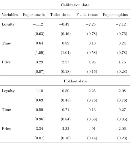
For the holdout and calibration data set we have the summary statistics in table 1 (in parenthesis, there are the standard deviations).
It is easy to see that the values differ only slightly for the calibration and holdout data set. Between the categories, there are large differences for all explanatory variables. The time variable has a huge standard deviation in all categories, this occurs due to many zeros, because the consumers did not buy in a category before.
Table 1 Summary statistics of the categories building the product bundles Calibration data
Variables Paper towels Toilet tissue Facial tissue Paper napkins Loyalty −1.12 −0.49 −2.25 −2.12
(0.63) (0.46) (0.78) (0.76)
Time 0.64 0.89 0.13 0.24
(1.09) (1.04) (0.58) (0.78)
Price 3.29 2.27 4.95 1.75
(0.07) (0.18) (0.16) (0.28) Holdout data
Loyalty −1.10 −0.50 −2.25 −2.08 (0.63) (0.45) (0.76) (0.76)
Time 0.59 0.71 0.13 0.27
(0.96) (0.84) (0.56) (0.85)
Price 3.34 2.32 4.91 2.06
(0.07) (0.16) (0.14) (0.23)
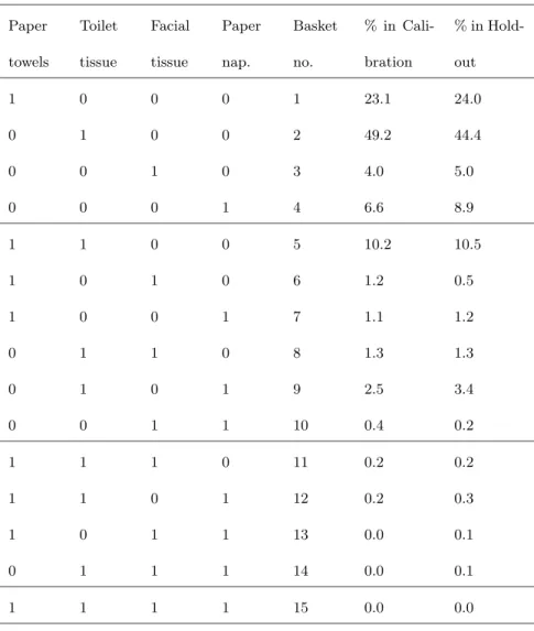
By modelling four product categories, we have 15 different market bas- kets as a possible result of a purchase trip. There are four baskets including only a single purchase, and all other baskets are described by a product bundle. We number the baskets as shown in table 2.
As you can see in table 2, the distribution between the calibration and holdout data set is very similar. A single purchase of toilet paper makes approximately half of all baskets. The portion of the basket with toilet pa- per and paper towels is twice as big as the single baskets including paper
Table 2 Market basket explanation and distribution Paper
towels
Toilet tissue
Facial tissue
Paper nap.
Basket no.
% in Cali- bration
% in Hold- out
1 0 0 0 1 23.1 24.0
0 1 0 0 2 49.2 44.4
0 0 1 0 3 4.0 5.0
0 0 0 1 4 6.6 8.9
1 1 0 0 5 10.2 10.5
1 0 1 0 6 1.2 0.5
1 0 0 1 7 1.1 1.2
0 1 1 0 8 1.3 1.3
0 1 0 1 9 2.5 3.4
0 0 1 1 10 0.4 0.2
1 1 1 0 11 0.2 0.2
1 1 0 1 12 0.2 0.3
1 0 1 1 13 0.0 0.1
0 1 1 1 14 0.0 0.1
1 1 1 1 15 0.0 0.0
napkins or facial tissues. The full basket is not purchased in any data set, and the baskets with three categories have only a very small part in all pur- chases. Here, we have a less strong distribution over all baskets as in Russel and Petersen (2000). Due to the different data situation, we may also get different estimation results.
4 Estimation results
Now we will describe the estimation results for the German data set. Before we will go into detail, we will compare three different model types to ensure that incorporating cross–effects will lead to better estimation results. First, we have a model without any cross–effect parameters (M1). This model can be seen as four single models for each category, where only the direct effects as PRICE, TIME, LOYAL and an intercept is included. The second stage of considering cross–effects is to include only the parametersδij, but with ignoring the SIZE effect (M2). The full models contains all variables mentioned before, including the SIZE effect (M3).
Table 3 Comparison of different models types with and without cross–effects Model # Param. Calibration LL Calibration AIC Holdout LL
M1 16 −1477.83 2987.65 −1097.63
M2 22 −1394.39 2832.78 −1043.26
M3 23 −1392.91 2831.81 −1042.66
As you can see in table 3, the full model gives significant better log- likelihood and significant better AIC values than the models with fewer parameters. We get here similar results to Russel and Petersen (2000). Ig- noring cross–effects leads to worse estimation. Now we will turn to the best model, the model with all cross–effects included and inspect their parameter estimation results.
In table 4, significance on the 5%–level is marked with∗∗, and for 10%
with∗. First, we will describe the results for the German data set. Later, we focus on the comparison of our results with the Canadian data set. In the German data set, the main effects are explained by the cross–effects withδ and by the loyalty of the consumers to a category. So we have a strong part of heterogeneity in the data set, which is shown through the strong effects of the HH estimations. But neither the time nor the price variable have any significant effect on explaining the choice behavior. These findings are stable over different parts of the data set. Also, the SIZE variable has a significant effect with a negative parameter estimate. We expected a positive sign for SIZE, because larger baskets are assumed to have a positive effect on the cross–effects. Regarding the non–significant estimates of time and price, we will try to modify the calculation of these variables to get significant effects with the right signs in a second step. As mentioned before in the paper, e.g. the TIME variable has often a zero value due to non–purchases in a specific category.
We will go not into detail in describing the estimation results for the Canadian data set, the reader is referred to Russel and Petersen (2000).
But we will compare the parameter values of the two data sets more in de- tail now. For the own effect parameters we have for loyalty similar results in both estimations regarding sign and significance. Only the magnitudes are different, which could be a tribute to non–standardization. The time param- eters in the German data set are quite large and not significant, contrary
Table 4 Parameter estimations for the full model including all cross–effects for the German and Canadian data set
Variable Paper t. Toilet p. Facial t. Paper n.
Own effects parameters
Intercept German data −2.057 3.007∗∗ −0.957 1.135 Canadian data 0.475∗ 0.310∗ −0.412∗ 0.250 Loyalty German data 1.019∗∗ 0.551∗∗ 1.998∗∗ 0.903∗∗
Canadian data 1.834∗∗ 1.667∗∗ 1.540∗∗ 1.849∗∗
Time German data 19.258 19.474 20.792 22.620 Canadian data 0.310∗∗ 0.184∗∗ 0.169∗∗ 0.884∗∗
Price German data 1.264 −0.363 0.739 0.172 Canadian data −0.730∗∗ −0.549∗∗ −0.957∗∗ −1.240∗
Cross–effect parameters
Size German data −0.354∗ −0.354∗ −0.354∗ −0.354∗ Canadian data 0.642∗∗ 0.642∗∗ 0.642∗∗ 0.642∗∗
Paper towels cross–effects G – −2.844∗∗ −2.111∗∗ −2.809∗∗
C – −0.657∗∗ −0.864∗∗ −1.174∗∗
Toilet paper cross–effects G −2.844∗∗ – −2.974∗∗ −2.901∗∗
C −0.657∗∗ – −0.763∗∗ −0.725∗∗
Facial Tissue cross–effects G −2.111∗∗ −2.974∗∗ – −2.340∗∗
C −0.864∗∗ −0.763∗∗ – −1.373∗∗
Paper napkins cross–effects G −2.809∗∗ −2.901∗∗ −2.340∗∗ – C −1.174∗∗ −0.725∗∗ −1.373∗∗ –
to the findings of Russel and Petersen (2000). Also, the price coefficients in the German data set do not deliver the nice results as the Canadian ones do. The differences in the cross–effect parameters are not as different as for the own effect. Here, we have mainly differences regarding the magnitudes of the parameters. Only for the size effect, we have negative signs in the German and positive ones in the Canadian results.
5 Summary and outlook
To model purchases not only in one category, but for a whole product bun- dle, it is necessary to use alternatives. One possible approach is to build a model on n–dimensional decisions, which can be related to each other.
Here, we use a multivariate logistic model which is estimated by methods of spatial statistics. Comparing the results of the German data with the ones of the Canadian study, we found strong effects for the cross–category vari- ables, but only non–significant ones for the base variables as price and time effect of purchases. The different results may have methodological reasons or may also be the result of cultural differences. The observations of Rus- sel and Petersen (2000) are only based on one city, but ours are for whole Germany and so may result in different consumer behavior.
Some variable specification as for price and time may be changed in a future study to get better results and to incorporated more individual effects. The inclusion of well established variables as feature and display should be made in a further step. Another direction of model extension is
to use non– or semiparametric models, as e.g. a generalized additive model (GAM) (Hastie and Tibshirani, 1990), which was also successfully used as an extension for a standard multinomial logit approach, as in Boztu˘g and Hildebrandt (2001) or Boztu˘g (2002).
References
B¨ocker F (1978) Die Bestimmung der Kaufverbundenheit von Produkten.
Duncker & Humblot, Berlin
Besag J (1974) Spatial interaction and the statistical analysis of lattice systems. Journal of the Royal Statistical Society, Series B 36 (2) 192–236 Boztu˘g Y (2002) Die Analyse der Preiswirkung auf die Markenwahl - Eine nichtparametrische Modellierung. Schriften zur quantitativen Betrieb- swirtschaftslehre. Deutscher Universit¨ats–Verlag, Wiesbaden
Boztu˘g Y, Hildebrandt L (2001) Nonparametric modeling of buying behav- ior in fast moving consumer goods markets. In: Papastefanou G, Schmidt P, B¨orsch-Supan A, L¨udtke H, Oltersdorf U (eds.) Social and Economic Research with Consumer Panel Data. ZUMA, Mannheim, pp. 189–205 Chib S, Seetharaman PB, Strijnev A (2002) Analysis of multi–category
purchase incidence decisions using IRI market basket data. In: Franses PH, Montgomery AL (eds.) Econometric Models in Marketing, vol. 16.
Elsevier Science, pp. 57–92
Cressie NAC (1991) Statistics for spatial data. John Wiley & Sons
Guadagni PM, Little JDC (1983) A logit model of brand choice calibrated on scanner data. Marketing Science 2 (3) 203–238
Hastie TJ, Tibshirani RJ (1990) Generalized Additive Models. Chapman
& Hall, London
Hruschka H (1985) Der Zusammenhang zwischen Verbundbeziehungen und Kaufakt– bzw. K¨auferstrukturmerkmalen. Zeitschrift f¨ur betrieb- swirtschaftliche Forschung 37 218–231
Hruschka H (1991) Bestimmung der Kaufverbundenheit mit Hilfe eines probabilistischen Meßmodells. Zeitschrift f¨ur betriebswirtschaftliche Forschung 43 (5) 418–434
Manchanda P, Ansari A, Gupta S (1999) The ”shopping basket”: A model for multicategory purchase incidence decisions. Marketing Science 18 (2) 95–114
Mild A, Reutterer T (2003) An improved collaborative filtering approach for predicting cross–category purchases based on binary market data. Journal of Retailing and Consumer Services 6 (4) forthcoming
Ratneshwar S, Pechmann C, Shocker AD (1996) Goal–Derived Categories and the Antecendents of Across–Category Consideration. Journal of Con- sumer Research 23 240–250
Russel GJ, Petersen A (2000) Analysis of cross category dependence in market basket selection. Journal of Retailing 76 (3) 367–392
Russell GJ, Bell D, Bodapati A, Brown CL, Chiang J, Gaeth G, Gupta S, Manchanda P (1997) Perspectives on multiple category choice. Marketing
Letters 8 (3) 297–305
Russell GJ, Ratneshwar S, Shocker AD, Bell D, Bodapati A, Degeratu A, Hildebrandt L, Kim N, Ramaswami S, h Shankar V (1999) Multiple–
category decision–making: Review and synthesis. Marketing Letters 10 (3) 319–332
Schnedlitz P, Kleinberg M (1994) Einsatzm¨oglichkeiten der Verbundanalyse im Lebensmittelhandel. Der Markt 33 (1) 31–39