Meteorology and oceanography of the Atlantic sector
of the Southern Ocean — a review of German achievements from the last decade
Hartmut H. Hellmer1&Monika Rhein2&Günther Heinemann3&Janna Abalichin4&
Wafa Abouchami5&Oliver Baars6&Ulrich Cubasch4&Klaus Dethloff7&Lars Ebner3&
Eberhard Fahrbach1&Martin Frank8&Gereon Gollan8&Richard J. Greatbatch8&
Jens Grieger4&Vladimir M. Gryanik1,9&Micha Gryschka10&Judith Hauck1&
Mario Hoppema1&Oliver Huhn2&Torsten Kanzow1&Boris P. Koch1&
Gert König-Langlo1&Ulrike Langematz4&Gregor C. Leckebusch11&Christof Lüpkes1&
Stephan Paul3&Annette Rinke7&Bjoern Rost1&Michiel Rutgers van der Loeff1&
Michael Schröder1&Gunther Seckmeyer10&Torben Stichel12&Volker Strass1&
Ralph Timmermann1&Scarlett Trimborn1&Uwe Ulbrich4&Celia Venchiarutti13&
Ulrike Wacker1&Sascha Willmes3&Dieter Wolf-Gladrow1
Received: 18 March 2016 / Accepted: 29 August 2016 / Published online: 16 September 2016
#The Author(s) 2016. This article is published with open access at Springerlink.com
Abstract In the early 1980s, Germany started a new era of modern Antarctic research. The Alfred Wegener Institute Helmholtz Centre for Polar and Marine Research (AWI) was founded and important research platforms such as the German permanent station in Antarctica, today called Neumayer III, and the research icebreakerPolarsternwere installed. The research primarily focused on the Atlantic sector of the Southern Ocean.
In parallel, the German Research Foundation (Deutsche Forschungsgemeinschaft, DFG) started a priority program
‘Antarctic Research’ (since 2003 called SPP-1158) to foster and intensify the cooperation between scientists from different
German universities and the AWI as well as other institutes in- volved in polar research. Here, we review the main findings in meteorology and oceanography of the last decade, funded by the priority program. The paper presents field observations and modelling efforts, extending from the stratosphere to the deep ocean. The research spans a large range of temporal and spatial scales, including the interaction of both climate components. In particular, radiative processes, the interaction of the changing ozone layer with large-scale atmospheric circulations, and chang- es in the sea ice cover are discussed. Climate and weather fore- cast models provide an insight into the water cycle and the Responsible Editor: Jörg-Olaf Wolff
* Hartmut H. Hellmer Hartmut.Hellmer@awi.de
1 Alfred-Wegener-Institut Helmholtz-Zentrum für Polar- und Meeresforschung, Bremerhaven, Germany
7 Alfred-Wegener-Institut Helmholtz-Zentrum für Polar- und Meeresforschung, Potsdam, Germany
8 GEOMAR Helmholtz-Zentrum für Ozeanforschung Kiel, Kiel, Germany
9 A.M. Obukhov Institute of Atmospheric Physics, Russian Academy of Sciences, Moscow, Russia
10 Institut für Meteorologie und Klimatologie, Leibniz Universität Hannover, Hannover, Germany
11 School of Geography, Earth and Environmental Sciences, University of Birmingham, Birmingham, UK
12 Ocean and Earth Science, National Oceanographic Centre Southampton, University of Southampton, Southampton, UK
13 Joint Research Centre (JRC) - European Commission’s Science Service, Brussels, Belgium
2 Institut für Umweltphysik IUP - Zentrum für Marine Umweltwissenschaften MARUM, Universität Bremen, Bremen, Germany
3 Environmental Meteorology, Universität Trier, Trier, Germany
4 Institut für Meteorologie, Freie Universität Berlin, Berlin, Germany
5 Max Planck Institut für Chemie, Mainz, Germany
6 Department of Geosciences, Guyot Hall, Princeton, NJ 08544, USA
climate change signals associated with synoptic cyclones.
Investigations of the atmospheric boundary layer focus on the interaction between atmosphere, sea ice and ocean in the vicinity of polynyas and leads. The chapters dedicated to polar oceanog- raphy review the interaction between the ocean and ice shelves with regard to the freshwater input and discuss the changes in water mass characteristics, ventilation and formation rates, cru- cial for the deepest limb of the global, climate-relevant meridio- nal overturning circulation. They also highlight the associated storage of anthropogenic carbon as well as the cycling of carbon, nutrients and trace metals in the ocean with special emphasis on the Weddell Sea.
Keywords Polar meteorology . Polar oceanography . Antarctica . Southern Ocean . Weddell Sea
Abbreviations
AABW Antarctic Bottom Water AAIW Antarctic Intermediate Water AAO Antarctic Oscillation
ABS Amundsen-Bellingshausen Sea ACC Antarctic Circumpolar Current AMPS Antarctic mesoscale prediction system AOGCM Atmosphere-ocean general circulation model AWI Alfred Wegener Institute Helmholtz Centre for
Polar and Marine Research CAO Cold air outbreak
CBL Convective boundary layer CDW Circumpolar Deep Water CFC Chlorofluorocarbon
COSMO Consortium of small-scale modelling CTD Conductivity-temperature-depth
DFG Deutsche Forschungsgemeinschaft (German Research Foundation)
DOC Dissolved organic carbon DOM Dissolved organic matter DWD German Meteorological Service
ECHAM General circulation model of the Max Planck Institute for Meteorology (Hamburg) EMAC ECHAM/MESSy Atmospheric Chemistry
ERA ECMWF reanalysis
ETC Extra-tropical cyclone
FESOM Finite Element Sea ice Ocean Model FRIS Filchner-Ronne Ice Shelf
GHG Greenhouse gas
HIRHAM Regional climate model combining HIRLAM and ECHAM
HIRLAM High-resolution limited area model HSSW High-Salinity Shelf Water
LES Large Eddy Simulation LIS Larsen Ice Shelf
MODIS Moderate-Resolution Imaging Spectroradiometer
NAM Northern Annular Mode
NCEP National Centres for Environmental Prediction NH Northern hemisphere
OA Ocean acidification
P-E Precipitation minus evaporation PACC Potential anthropogenic climate changes SAM Southern Annular Mode
SAMW Subantarctic Mode Water SH Southern hemisphere SIC Sea ice concentration SIE Sea ice extent
SPP Schwerpunktprogramm (DFG Priority Program) SZA Solar zenith angle
UV Ultraviolet
WDW Warm Deep Water
WMO World Meteorological Organization WSBW Weddell Sea Bottom Water WSDW Weddell Sea Deep Water
1 Introduction
Two hundred years ago, the Southern Ocean was viewed as an inaccessible, stormy and icy sea, challenging dauntless explorers, hunters and whalers. Today, the Southern Ocean is considered to be an important tessera of the climate puzzle hosting numerous processes of global importance. It connects the three major oceans through the most vigorous ocean current on Earth, the Antarctic Circumpolar Current, ventilates most of the world ocean abyss, participates in the global carbon cycle and affects the rate of global sea level rise due to the interaction with the Antarctic Ice Sheet. However, the Southern Ocean not only acts but also reacts to sea floor topography and the polar atmosphere.
The former guides currents around the continent, warm waters of open ocean origin into ice shelf cavities, dense shelf waters down the continental slope and determines the kind of water able to escape the basins of the marginal seas. The latter provides energy for driving the ocean currents, controls the surface fluxes of heat and moisture, regulates the exchange of natural and anthropo- genic gases and determines sea ice properties and coverage with consequences for primary production, ocean-air fluxes and water mass characteristics. The atmosphere links air-ice-ocean interac- tion with the stratosphere, e.g. changes in stratospheric circula- tion, due to ozone loss, to tropospheric circulations and sea ice coverage. Furthermore, the atmosphere is the fastest connection between Antarctica and the mid-latitudes, and the tropics.
It is the interplay between both components of the climate system, which restricts scientific surveys in the Southern Ocean mainly to the austral summer season, and even then, the access to the continental shelves of the marginal seas is limited. The combination of results from the few expeditions
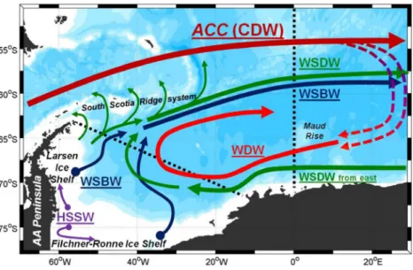
to the Antarctic coast, the increasing capability of satellite sensors, and the progress achieved in terms of numerical mod- el development revealed that the continental shelves are the prime locations for sea ice formation due to intense ocean heat loss to the cold atmosphere. Concentrated in coastal polynyas, the resulting brine rejection causes a densification of the con- tinental shelf water. This water mass either contributes to the formation of deep and bottom water or participates in the sub- ice shelf circulation providing the heat for basal melting. The meltwater input influences the stability of the shelf water col- umn with consequences for sea ice cover, for air-sea fluxes and for the characteristics of the deep and bottom waters. The main source region for both water masses is the southern ex- treme of the Atlantic Ocean, the Weddell Sea (Fig.1). Due to the ocean ridges fringing the Weddell Basin, only Weddell Sea Deep Water escapes via several deep passages and feeds the Antarctic Bottom Water, historically assumed to be the source for most of the abyssal waters.
Due to the potential of the Weddell Sea region for innova- tive discoveries and the relative vicinity to home ports, past (W. Filchner,DeutschlandExpedition, 1911–1913) and recent German investigations focussed on the Weddell Sea and the fringing continent including ice shelves and the hinterland.
Since 1981, continental research in the Weddell Sea area is based on theEkstrømisenat the German permanent station, today called‘Neumayer III’, and the summer Kohnen Station on Drauning Maud Land (Fig.1). Since 1982, expeditions to the Weddell Sea (and beyond) are supported immensely by the icebreakerPolarstern, which provides the platform for multi- disciplinary polar research even during the austral winter
months. Two research aircraft are available for scientific cam- paigns during the summer season. These research platforms (stations, icebreaker, aircraft) are run by the Alfred Wegener Institute Helmholtz Centre for Polar and Marine Research (AWI) and allow the operation of modern devices ranging from ROVs to recently used unmanned air vehicles (UAV, Jonassen et al.2015) for atmospheric boundary layer research.
Here, we review the achievements of recent investigations of the polar atmosphere and ocean with the focus on the Weddell Sea, primarily funded by the Priority Program (Schwerpunktprogramm, SPP-1158)‘Antarctic Research’of the German National Science Foundation (Deutsche Forschungsgemeinschaft, DFG). The main aim of the SPP is to give scientists from universities access to Antarctic stations and research platforms, thereby fostering and intensifying the cooperation between scientists from different German univer- sities and the AWI as well as other institutes worldwide in- volved in polar research. This paper summarizes the main findings of the last decade.
2 Climate relevant processes in the Antarctic atmosphere
The atmosphere is a key component of the Antarctic climate system. Atmospheric processes ranging from micrometres to thousands of kilometres are responsible for the interaction and transports of momentum, energy and matter at the interface of ocean and ice surfaces, exchange between tropics, mid-latitudes and the Antarctic and the exchange between stratosphere and
Fig. 1 Map of the Atlantic Sector of the Southern showing bottom topography, trajectories of warm deep water (WDW,red), Weddell sea deep water (WSDW,dark blue), Ice shelf water (ISW,light blue), and low-salinity shelf water (LSSW,green). Locations of one historic (Forster) and the two re- cent German stations on the con- tinent asblue dots.Abbreviations used are listed in theinsert
troposphere. Research in the realm of the Antarctic atmosphere contributed to the understanding of the interaction of the chang- ing ozone layer with large-scale atmospheric circulations and changes in the sea ice cover (Section2.1). The complex inter- action between the radiation field as a function of wavelength, snow reflection and clouds was investigated (Section 2.2).
Studies using climate and weather forecast models improved knowledge of the climate change signals associated with syn- optic cyclones (Section2.3) and the water cycle (Section2.4).
Investigations of the atmospheric boundary layer focused on the interaction between atmosphere, sea ice and ocean particularly for leads and polynyas (Section2.5).
2.1 Ozone-related changes in atmospheric circulation and sea ice extent
The stratospheric ozone depletion is most evident in the ozone hole that appears each austral spring over Antarctica. The ozone depletion led to a 6 °C cooling of the lower stratosphere over the South Pole and an associated intensification of the stratospheric vortex in spring. The interaction of these strato- spheric changes with the troposphere and particularly with the sea ice extent in the Antarctic was a focus of international research during the last decade. Since 1992, weekly ozone soundings have been performed at the German Antarctic re- search station Neumayer (König-Langlo and Loose,2007).
These measurements continue the time series that started al- ready in 1985 at the neighbouring German research base Georg-Forster-Station (König-Langlo and Gernandt, 2009).
Ozone sensors (ECC 5A/6A) mounted on RS80/RS90/RS92 radiosondes (Vaisala) have been used. High ozone partial pressures are measured at altitudes around 20 km—called
‘ozone layer’—from December/January to the end of August. During Antarctic spring (September to November), the ozone layer vanishes more or less completely.
This Antarctic springtime ozone depletion shows remark- able interannual variations (Fig.2). From 1985 to about 2006, an overall reduction of the ozone partial pressure in the ozone layer is obvious. The ozone reduction is strongly correlated with a cooling of the stratosphere. Corresponding variations or a significant trend during other seasons could not be ascertained. A biennial oscillation of the springtime ozone concentrations is evident from 1985 until 1989. Labitzke and Van Loon (1992) explained this behaviour as dynamically induced from the quasi-biennial oscillation of stratospheric wind above the equator. In the 1990s, the biennial oscillation of the spring ozone concentration was not measured any lon- ger. The data showed a more or less continuous reduction of the ozone concentration and a cooling of the air around 70 hPa. Crutzen and Arnold (1986) explained this behaviour as a chemical effect caused by the worldwide rising anthropo- genic chlorofluorocarbon (CFC) concentrations.
Between 2001 and 2004, the overall springtime ozone con- centrations measured above an altitude of 20 km were rising again. This effect was interpreted as the beginning of the re- covery of the‘ozone hole’as a response to the worldwide ban of nearly any CFC product in the Montreal Protocol in 1987.
However, the measurements in the following years from Neumayer II (Hoppel et al.2005) showed that the recovery of the ozone hole did not start at that time. Especially the very high temperatures and ozone concentrations during Spring 2002 (Fig.2) could be explained as a consequence of a dy- namic breakdown of the Antarctic stratospheric vortex during winter. It took a whole decade until the measurements from Neumayer and other Antarctic stations indicated an ongoing recovery of the ozone layer. In September 2014, the World Meteorological Organization (WMO) officially posted the success of the Montreal Protocol from 1987 (WMO2014).
However, the observed increase of global annual mean total ozone of 1 % between 2000 and 2013 compared to the large
Fig. 2 Time series of the average ozone partial pressure (red) and temperature (blue) at 70 hPa at the stations Georg-Forster and Neumayer covering the period 1985 to 2014
interannual variability found in that time period did not allow to conclude a recovery of the Antarctic ozone.
The trends of sea ice extent (SIE) during the last decades are different for both hemispheres. Arctic sea ice has dramat- ically decreased in the recent past. Estimates from satellite measurements find a negative trend of about 10 % per decade since 1979 (Comiso et al.2008). In contrast, annual mean Antarctic sea ice increased by about 1 % per decade for the years 1978–2006 (Turner et al.2009). While the Arctic sea-ice retreat has been associated with the warming of the tropo- sphere caused by increasing greenhouse gas (GHG) concen- trations (IPCC2013), the ozone depletion by man-made hal- ogens in the polar stratosphere and its impact on tropospheric circulation have been suggested as the driving mechanism to explain the observed Antarctic changes (e.g. Thompson and Solomon2002). However, there is still low confidence in the scientific understanding of the observed increase in Antarctic SIE since 1979, due to missing knowledge of internal variabil- ity and competing explanations for the causes of change (IPCC2013). With further increasing GHGs and an expected recovery of polar ozone at the end of the twenty-first century, projections of future polar climate and its hemispheric differ- ences are highly uncertain. To understand and project the in- teractions between the atmosphere, oceans and the cryosphere as well as the chemical and radiative effects of natural and anthropogenic climate gases throughout the troposphere and stratosphere, complex numerical models need to be applied. A new atmosphere-ocean version of the ECHAM/MESSy Atmospheric Chemistry (EMAC) chemistry-climate model was used in a study, which combines the EMAC model (Jöckel et al. 2006) with the Max Planck Institute-Ocean Model (MPI-OM, Jungclaus et al.2006).
The coupled atmosphere-ocean system is characterized by unforced internal variability on different time scales, as is evident in a 110-year EMAC simulation that was inte- grated under fixed boundary conditions for the year 1960.
The analysis begins for austral winter (June/July/August, JJA), using the Southern Annular Mode (SAM) index at 850 hPa and JJA mean SIE around Antarctica. The SAM is the dominant mode of low frequency variability in the southern hemisphere atmosphere, a positive/negative SAM being associated with stronger/weaker westerly winds (Thompson and Wallace 2000). The analysis re- veals a positive correlation between the SAM index and SIE on interannual time scales, while a significant corre- lation at low frequencies was not found (Fig. 3). The positive correlation between the SAM and SIE at interan- nual time scales is consistent with observations. It has been suggested to result from stronger westerlies during positive SAM that insulate the high latitudes from ex- change with the lower latitudes and lead to an overall cooling of the Antarctic region, even though some areas may also experience higher temperatures and less sea ice
during a positive SAM like the Antarctic Peninsula (e.g.
Thompson and Solomon2002). However, the lack of cor- relation between the SAM and SIE at low frequencies in the model does not support the hypothesis that the ob- served trend towards the positive polarity of the SAM can explain the observed increase in sea ice.
A comparative analysis of the Arctic region reveals a sim- ilar behaviour on interannual time scales (not shown) in which the SIE is positively correlated with the Northern Annular Mode (NAM)—the northern hemisphere equivalent of the SAM—consistent with previous studies (e.g. Rigor et al.
2002). However, on time scales longer than 11 years a much more coherent pattern of behaviour emerges in which periods of a positive polarity of the NAM are associated with reduced SIE and vice versa (not shown). This happens because the NAM is an important driver for the Atlantic meridional overturning circulation (Eden and Jung2001); and on time scales longer than 11 years, an enhanced overturning warms the high northern latitudes leading to reduced SIE.
Figure 4a shows the evolution of Antarctic SIE between 1960 and 2100, as simulated with the EMAC model assuming a continuing future increase of GHG concentrations according to the RCP6.0 scenario (IPCC2013) and projected emissions of ozone depleting substances following the WMO A-1 sce- nario. During the period of strongest Antarctic ozone deple- tion (about 1980–2007), the SIE shows considerable interan- nual variability but no indication of a retreat comparable to the Arctic. The local changes in sea ice concentration (SIC) around Antarctica in this period agree with observations (e.g. Turner et al. 2009): Consistent with an intensification of the Amundsen-Bellingshausen Sea (ABS) low, enhanced northerly winds induce a reduction of SIC in the ABS, while stronger southerlies lead to a larger SIC in the Ross Sea. An even stronger SIC enhancement was found in the Weddell Sea (left panel in Fig.4b). These changes arise from two contri- butions: (a) an increase of the SAM associated with the inten- sification of the stratospheric polar vortex during Antarctic ozone depletion and a concurrent reduction in planetary wave activity and (b) enhanced synoptic activity due to climate change. In the upcoming decades (2008–2054, middle panel in Fig.4b), i.e. a period with increasing climate change and declining yet still relevant ozone depletion, the SIC increases over the Ross and Weddell Seas are weaker. However, in the second half of the twenty-first century (2055–2096, right pan- el in Fig.4b), when total column ozone is projected to recover, the GHG induced climate change will dominate and Antarctic SIC is projected to reduce, similar to the Arctic. While the spatial signatures of past SIE changes in EMAC are consistent with observations, the largest modelled changes occur in aus- tral winter and spring, in contrast to autumn in the measure- ments. More analysis is also required to separate and quantify the relative impacts of ozone and GHG changes on Antarctic sea ice and, in general, polar climate.
2.2 Progress in the measurements of sky luminance and sky radiance
Variations in the ozone concentrations have a strong impact on the incoming radiation on the earth surface. It is well known that the direct impact is strongly wavelength-dependent.
While the influence of ozone concentrations on the radiation is weak in the visible part of the spectrum, it can be dominant in parts of the infrared and in the shortwave ultraviolet (UV) spectrum. An improved understanding of the radiation is therefore helpful to determine the impact of current and future changes on the climate in Antarctica. Angular distribution of solar radiance and its spectral characteristics are key radiative quantities to study the impact of climate changes in Antarctica (Cordero et al.2013,2014). These quantities and the absorp- tion characteristics of snow determine how much radiation is reflected back to space and how much snow melts should temperatures rise.
In the last decade, the observational capabilities for mea- suring radiance and luminance were significantly improved.
In contrast to the‘old’scanning instruments that needed one day to measure the spectral radiance field, the newly devel- oped instruments are now capable to measure sky radiance in dependence of zenith and azimuth angle in more than 100 directions simultaneously within a second (Riechelmann et al. 2013; Tohsing et al. 2013; Seckmeyer et al. 2010).
These instruments have already improved our understanding of climate change in both the Arctic and Antarctic, and we expect that also for the future.
Sky luminance and spectral radiance have been character- ized at the Neumayer Station during the austral summer 2003/
2004 (Wuttke and Seckmeyer2006). The high reflectivity of the surface (albedo) in Antarctica, reaching values up to 100 % in the UV and visible part of the solar spectrum due to snow cover (Wuttke et al.2006) modifies the radiation field considerably when compared to mid-latitudes. A dependence Fig. 3 aNormalized JJA mean
time series of the southern hemisphere sea ice extent SIE (i.e.
SIE is divided by its interannual standard deviation, about 0.9 × 10⁶km2) and the SAM (defined as in Thompson and Wallace2000) in the control run of EMAC-O-CCM.b11-y run- ning means using Hamming win- dow.cShows (a) minus (b).
Correlation values between the time series are indicated in the upper leftof each panel
of luminance and spectral radiance on solar zenith angle (SZA) and surface albedo was identified. For snow and cloud- less sky, the horizon luminance exceeds the zenith luminance by as much as a factor of 8.2 and 7.6 for a SZA of 86° and 48°, respectively. Thus, a snow surface with high albedo can en- hance horizon brightening compared to grass by a factor of 1.7 for low sun at a SZA of 86° and by a factor of 5 for high sun at a SZA of 48°. Measurements of spectral radiance show in- creased horizon brightening for increasing wavelengths and, in general, a good agreement with model results. However, large deviations are found between measured and modelled values especially in the infrared range that are only partly explained by measurement uncertainties. Progress is expected by future studies with the faster instruments available now.
2.3 Extra-tropical cyclones and storms and their impact on the southern polar hemisphere
Extra-tropical cyclones (ETCs) in the mid to high latitudes of the southern hemisphere (SH) are a fundamental part of the atmospheric energy and momentum transport. ETCs are es- sential for the meridional exchange processes, which are nec- essary to maintain the hemispheric and, thus, global energy balance of the Earth’s climate system. In contrast to the north- ern hemisphere, where stationary waves in the mid-
troposphere are important for the poleward energy transport, the atmospheric energy transport in the SH is mainly accom- plished by transient and shorter baroclinic waves, evident as travelling ETCs at the surface. In the absence of orographic influences, which lead to distinct areas of baroclinic cyclogen- esis in the northern Atlantic and Pacific, the SH transient waves have a more circumpolar distribution. At present, po- tential anthropogenic climate changes (PACC) are investigat- ed by means of a multi-model ensemble of state-of-the-art coupled atmosphere-ocean general circulation model (AOGCM) simulations, especially to understand the nature and causes of potential changes in future ETCs and their im- pact on Antarctica.
Most individual models as well as the ensemble mean are able to reproduce the general ETC characteristics of the SH.
Nevertheless, a large model-to-model variability is revealed with respect to the quantity of simulated ETCs. Grieger et al.
(2014) used a new scaling approach to account for these sys- tematic biases. Applying the SRES A1B scenario (e.g.
Nakicenovi et al.2000) the total number of cyclones decreases at the end of the twenty-first century (due to stronger warming of the lower troposphere in polar regions one would expect less net energy transport). However, the majority of analysed AOGCMs (Fig.5) diagnose an increased number of extremely strong ETCs. This general change is associated with a Fig. 4 aEvolution of the Antarctic total ozone column (in Dobson Unit,
DU, 60° S–90° S mean,black) in October and Antarctic sea ice extent (SIE, in km2,blue) in December between 1960 and 2100, simulated with the EMAC chemistry-climate model, assuming the RCP6.0 greenhouse gas scenario and the WMO-A1 scenario for ozone depleting substances.
The time series have been smoothed by applying three times a 1-2-1 filter.
bDecadal trends in sea ice concentration (SIC) in October for the periods 1980–2007 (left), 2008–2054 (middle), and 2055–2096 (right). Grid box- es with SIC >0.15 are considered as covered with sea ice
poleward shift related to upper tropospheric tropical warming and shifting meridional sea surface temperature gradients in the Southern Ocean (Grieger et al.2014). The largest increase of strong cyclone activity was found in the eastern hemisphere.
The potential anthropogenic climate change also im- p a c t s p o l e w a r d m o i s t u r e f l u x e s i n t h e S H . Distinguishing between thermodynamic and dynamic in- fluences of PACC on moisture fluxes, PACC signals of the responsible waves in the synoptic scale show a pole- ward shift related to the poleward shift of ETCs (Grieger et al.2015). Antarctic net precipitation was calculated by means of the vertically integrated moisture flux. Grieger et al. (2015) found signals of increasing net precipitation whereas the dynamical part of net precipitation decreased.
They explained these findings with the low variability of synoptic-scale waves, which generally decreased, espe- cially off the coast of West Antarctica, and suggested that this is related to a changing variability of the ABS low.
Another factor potentially changing Antarctic surface cli- mate, is the SH springtime ozone depletion since the mid- 1980s. It has its strongest impact during the austral summer months (DJF) due to a slow downward propagation of ozone hole induced anomalies in temperature, geopotential height, and wind fields. Stronger zonal surface winds were supposed to isolate the Antarctic vicinity, inducing a cooling signal in
surface temperature (Gillett and Thompson, 2003).
Simulations with the ECHAM/MESSy Atmospheric Chemistry model show, however, an enhancement of Antarctic surface temperature in the recent past (1960 to 2000) (Fig.6, top left). The warming of the Antarctic surface climate, which is in good agreement with recently published observational studies (Steig et al.2009; Schneider et al.2012), is due to climate change by increasing GHG concentrations. It is found to be a consequence of enhanced meridional heat transport by synoptic waves (Fig.6, top right), associated with an increased storm track density around Antarctica (not shown). The contribution to the heat flux by planetary waves (Fig.6, top middle), however, is strongly reduced (consistent with stronger zonal winds, Fig.6, top left). Due to the occur- rence of the ozone hole, synoptic heat fluxes near the surface are suppressed, and the decrease in the planetary heat flux throughout the troposphere predominates (Fig. 6, lower middle), leading to a subsequent cooling of the continent.
These results illustrate a counteraction of different climate drivers (enhanced sea-surface temperatures due to climate change and recurring springtime ozone hole), leading to a two-way impact on the characteristics of SH extra-tropical waves with a more or less pronounced enhancement of syn- optic heat transport. However, more impacts have to be taken into account to fully explain the observed recent Antarctic surface changes, such as reduced radiative input due to cloud Fig. 5 Relative climate change signal [%] of the multi-model ensemble cyclone track density (April–September) for all (left) and strong (right) cyclones.
Stippled areas indicate significant changes (p< 0.05) with respect to a Student’sttest (Figure adopted from Grieger et al.2014)
cover changes with increased cyclone activity, or changes in regional wind systems, such as katabatic winds.
2.4 Components of the water cycle and their role for ice and snow accumulation
Precipitation is the dominant term among the various compo- nents of surface snow accumulation. Information from in situ observations for precipitation events are hardly available due to the difficulties in measuring precipitation under Antarctic conditions, even when using automatic weather stations (e.g.
van den Broeke et al.2004; Welker et al.2014). Therefore, an annual snow accumulation climatology has been frequently used as an indicator for precipitation (King and Turner 1997). Later on, precipitation climatologies have been derived from model data, such as reanalysis data (Bromwich et al.
2011), mesoscale weather forecasts using the Antarctic Mesoscale Prediction System (Bromwich et al.2005) as shown by Schlosser et al. (2008) or by regional climate models (van de Berg et al. 2006; Lenaerts et al. 2012).
Recently, Palerme et al. (2014) have used satellite products from CloudSat to derive precipitation. Highest precipitation rates of more than 500 mm per year were found along the
coastal escarpment; on the ice sheet plateau, the rates drop to less than 100 mm per year.
2.4.1 Precipitation processes related to synoptic disturbances
Large portions of precipitation in the coastal regions fall dur- ing episodes of passing fronts of cyclonic systems (King and Turner 1997). If precipitation, and hence the accumulation, occurs preferentially during particular months of the year, the temperature derived from ice core analysis will be biased towards the conditions prevailing during these days in the region around the drilling site. Thus, it is necessary to know the amount and timing of precipitation and to investigate pre- cipitation events on short time scales with high spatial resolution.
A high spatial and temporal resolution is needed particu- larly for the simulation of high precipitation events. A selected weather situation, formation and horizontal distribution of clouds and precipitation in Queen Maud Land have been in- vestigated by Wacker et al. (2009), using a high-resolution non-hydrostatic weather forecast model COSMO (consortium of small-scale modelling; Steppeler et al.2003). This model was initially developed at the German Meteorological Service (DWD) and applied in that study for the first time for Antarctic Fig. 6 Past changes (1960–2000) in surface temperature and wind [in K
and m/s,left panels], zonal mean heat flux from planetary (middle panels) and synoptic (right panels) waves [in km/s] in DJF.Blue shadesdenote a cooling in surface temperature and an enhancement in heat fluxes. The
analyses are based on 20-year time slice simulations under respective conditions. Thetop rowshows the climate change signal due to rising GHGs and stratospheric ozone depletion. Thebottom rowshows the response to stratospheric ozone depletion only
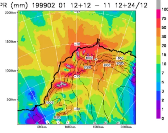
conditions. A 12-day episode from February 1999 is ad- dressed, when low-pressure systems and related fronts trav- elled along the coast of Queen Maud Land. Emphasis was placed on the temporal evolution and horizontal distribution of clouds and precipitation in high spatial resolution (7-km horizontal mesh size).
The model captures the overall meteorological situation.
The horizontal distribution of 12-day precipitation sums is shown in Fig. 7. The amount of modelled precipitation, in particular sums larger than 100 mm in some regions with steep topography, seems to be large when compared to the annual climatologies and to simulations with the Antarctic mesoscale prediction system (AMPS) or ECMWF reanalysis (ERA)- Interim reanalysis (Welker et al.2014). The spatial precipita- tion distribution is dominated by topographic effects:
Precipitation amount generally decreases towards the interior similar as seen in climatologies. In the high-resolution simu- lation, however, the decrease neither follows increasing dis- tance from the coast nor the topographic contours. Instead, precipitation bands of some 100-km width appear on the pla- teau. The bands may be connected to the path of the frontal cloud systems, and may also be related to orographically in- duced gravity waves (see e.g. Zaengl2005), which have been studied for long for Antarctica. Such mesoscale features can only be resolved by models with mesh sizes of 10 km or less (e.g. Valkonen et al.2010).
Figure8shows time series of 6-h precipitation at a partic- ular grid point close to Neumayer Station from the study of Wacker et al. (2009). The simulated timing of precipitation
agrees with synoptic observations. The figure also illustrates some of the difficulties in precipitation modelling. The precip- itation amount during the first 6 h of the forecast is systemat- ically underestimated due to the spin-up effect. Even beyond the spin-up period two successive model runs clearly differ in the amount of precipitation falling in the overlapping period.
Without observational data, we cannot tell which one is more reliable.
All mentioned studies on precipitation in Antarctica using mesoscale forecast models, show some success in the simula- tion of general spatial and temporal patterns. Nevertheless, all model precipitation data for Antarctica reveal deficiencies, such as the supposed overestimation (Fig.8). This argues for a continuing effort in both numerical model development and precipitation observations.
2.4.2 Regional climate model simulations of the water cycle
Regional climate model (RCM) simulations based on HIRHAM4 (regional climate model combining high- resolution limited area model (HIRLAM) and ECHAM) have been carried out over Antarctica laterally driven by European Reanalysis data ERA-40 for four decades be- tween 1958 and 1998. The model simulations with a hor- izontal resolution of 50 km provide a relative realistic simulation o f the mean atmospheric circulation, baroclinic-scale weather systems, and the spatial distribu- tion of precipitation minus sublimation structures (Dethloff et al. 2010). The associated atmospheric
Fig. 7 Horizontal distribution of simulated precipitation sums (in mm water equivalent) for the period 2 February 12 UTC to 13 February 00 UTC, taken from successive COSMO- model runs.
The runs started on 1 to 11 February 1999 each at 12 UTC.
The first 12 h of each simulation are skipped as spin-up time. From Wacker et al. (2009), Figure 13b.
Copyright Cambridge University Press, reprinted with permission
circulation and synoptic variability of the model agree with that of ERA-40, however with a pronounced internal variability (Xin et al.2010). The computed precipitation minus evaporation (P-E) trends describe the observed
surface mass accumulation increase at the West Antarctic coasts and reductions in parts of East Antarctica (Fig. 9).
The regional accumulation changes are largely driven by changes in the transient activity around the Antarctic coasts due to the varying Antarctic oscillation (AAO) phases. The monthly mean AAO index from 1958 to 1998 is based on the first principal component of the National Centres for Environmental Prediction (NCEP) 850 hPa extratropical height field (20° S–90° S) adapted from Thompson and Wallace (2000). During positive AAO, more transient pres- sure systems travel towards the continent; thus, West Antarctica and parts of southeastern Antarctica gain more pre- cipitation and mass. Over central Antarctica, the prevailing anticyclone causes a strengthening of polar desertification connected with a reduced surface mass balance in the northern part of East Antarctica. The shifts in the AAO pattern is ac- companied by changes in the short baroclinic waves. The associated heat and humidity fluxes (on time scales 2–6 days at 850 hPa) between positive and negative AAO periods show most pronounced shifts over the Southern Ocean. During pos- itive AAO phases, increased heat and humidity transports, due to synoptical cyclones towards the Antarctic continent, appear over the Pacific Ocean, while over the Atlantic Ocean a re- duction occurs (Dethloff et al.2010).
2.5 The atmospheric boundary layer and interactions with sea-ice and ocean
The grid size of the newest generation of weather prediction models reaches the kilometre range and might decrease in the future to even smaller values, approaching finally the scale of Fig. 8 Time series of simulated 6-h precipitation sums (in mm water
equivalent; allocated to the final time of the period), valid at a model grid point near Neumayer Station. Results are plotted for the 48-h simulation period from COSMO model runs as used for Fig.7. Start of a new run is marked by asquare. Successive runs are plotted alternatively asblack solidandred dashed lines.Asterisksmark whether the synop data report precipitation (yes >0, no =0), but they do not indicate the amount of precipitation; cases of blowing/drifting snow are excluded. Copyright Cambridge University Press, reprinted with permission
Fig. 9 Annual accumulation trends (mm/year2) for 1992–2001 based on HIRHAM simulations.
The areas of significant positive or negative changes with 95 % confidence are indicated.White regionsdescribe areas below the 95 % significance level
large convective eddies in very shallow convection. The turbu- lent processes at grid sizes around 1 km become partly resolved and partly parameterized. When flux parameterizations in this overlapping region (often called grey zone or terra-incognita;
Wyngaard (2004); Mironov (2009)) are not adjusted to the higher resolution, fluxes can be double-counted. Studies on convective mesoscale processes that occur frequently in both polar regions are presented in the following with a special focus on the difficulties related to the grey-zone problem. Due to the similar environment, process studies that have been carried out in the Arctic are very relevant for the Antarctic as well.
2.5.1 Convection over leads
The atmospheric boundary layer over closed polar sea ice is often characterized by a near-neutral or slightly stable layer of 100–300-m thickness, capped by a strong inversion. Radiative cooling or warm-air advection can even lead to surface-based inversions. However, also convective processes can occur over small cracks in sea ice, which often widen to channels or lake-like openings (leads; Fig.10). Over leads, the large difference between air and sea surface temperature generates strong convective plumes, which interact with the stably strat- ified environment (see, e.g. the review paper by Vihma et al.
(2014)). The strong unstable stratification over the leads with Obukhov lengths down to 0.11 m (Andreas and Cash1999) causes heat fluxes (up to several hundred W m−2). Therefore, they have to be taken into account in the calculation of the surface energy budget even when the area fraction of leads is often not greater than 1–5 %. Although the effect of single leads can be small, the integral effect of a lead ensemble in a large region can increase the near-surface temperature of a drifting air parcel by several Kelvin when the sea ice concen- tration changes by 1 % only (Lüpkes et al.2008a).
Thus, it is important to account for convection over leads in climate models. The horizontal scale of leads and plumes is much below the grid size of climate models so that the fluxes over grid boxes with partial sea ice coverage usually depend
linearly on the sea ice concentration. However, Andreas and Cash (1999) emphasize that fluxes per unit area are larger over small leads than over large ones, and Lüpkes and Gryanik (2015) show that the transfer of momentum and heat depends nonlinearly on sea ice concentration.
The treatment of convection over leads is not only difficult with respect to surface fluxes, the processes above the surface layer are also complex as shown by, e.g. Lüpkes et al. (2008b) and Esau (2007). One reason is the strong horizontal non- homogeneity related to the developing plume, which consists of thermals drifting with the mean wind. The inclination of this plume (Fig.11) depends on wind and the buoyancy flux. While there are large upward heat fluxes within the plume, cooling over ice causes also a slightly stably stratified layer with small downward heat fluxes below the plume. Lüpkes et al. (2008b) used the Large Eddy Simulation (LES) model PALM with 10- m grid size for a detailed modelling of the turbulent processes over leads and compared the results with those of the mesoscale model METRAS (Schlünzen1990). The latter was run with a grid size of 200 m, which resolves the plume but not the smaller eddies (thermals) as the LES does. A good agreement of both model results could only be obtained when METRAS was used with a new turbulence closure accounting for the effects of horizontal non-homogeneity caused by the convective plume.
It combines a local closure outside the plume region with a non- local closure inside the plume. For the non-local closure, a new scaling was suggested which is based on the vertically integrat- ed mean horizontal velocity at the lead’s upstream edge, on the surface buoyancy flux over the lead, and on the internal con- vective boundary layer height (upper boundary of plume). In contrast, the traditional scaling assuming horizontal homogene- ity did not work for this resolution.
The application of the new closure showed that regions of down-gradient transport and counter-gradient transport are well reproduced as in the corresponding LES (Fig. 11).
Hence, a good agreement resulted also for the wind and tem- perature fields (see Lüpkes et al.2008b), which were strongly affected by the convection over leads. These investigations
Fig. 10 Lead observed over the Barents Sea near Svalbard in April 2007 (Photo: C. Lüpkes). Its estimated width is 100 m. Due to relatively warm air temperatures around−10 °C only very little sea smoke, often indicating the convective plume, developed here
show that the above parameterizations can be considered as a first step towards an adjustment of convection parameteriza- tions to the grey zone in case of shallow convection over leads. Forthcoming climate models should account for the nonlinear dependence of fluxes on the sea ice concentration.
2.5.2 Cold-air outbreaks
Processes over leads can influence the inner polar ocean re- gions and the marginal sea ice zones, but during cold-air out- breaks (CAOs) energy fluxes of similar magnitude occur also over wide ocean regions with open water. Then, strong roll convection develops and the atmospheric boundary layer height increases from roughly 100 m over the polar marginal sea ice zone to 1–2 km in a far distance (Fig.12). Several 100 km downstream of the ice edge, typically, a transition from roll to cellular convection takes place.
The patterns of organized convection, which are visible by cloud streets, are observed over Greenland and the Barents
Sea in more than 50 % of the time during winter (Brümmer and Pohlmann 2000). Although similar statistics for the Antarctic are not yet available, satellite images show that CAOs with organized convection are a frequent phenomenon during off-ice flow, e.g. over the Bellingshausen Sea. Studies of CAOs in the Arctic can be considered as representative also for the Antarctic. Due to their impact on the exchange pro- cesses between ocean and atmosphere, it is important that they are well represented by parameterizations used in numerical weather and climate models.
Several studies (e.g. observational studies by Brümmer 1999; Hartmann et al.1997) show that roll convection can substantially contribute to vertical transport of heat, moisture, and momentum. Therefore, it is often argued that vertical transport might be enhanced by rolls (e.g. Kristovich et al.
1999). However, as discussed in Gryschka et al. (2014), this needs to be proven. One reason is that it is not possible to find an observed reference case without rolls for the same large- scale forcing. A second reason is that, so far, it was assumed Fig. 11 The convective plume
region over a lead (position between 0- and 1-km distance) is shown for two wind speeds (left U= 3 m/s,right U= 5 m/s) roughly as the region bounded by the 0-contour line. Also, regions with heat fluxes along the gradi- ent of potential temperature (black area) and with counter- gradient fluxes (white area bounded by the 0-contour) are shown as modelled with the LES PALM (top) and with the meso- scale model METRAS (bottom).
Figure from Lüpkes et al. (2008b)
Fig. 12 Schematic figure of roll convection and cloud streets during a CAO derived from a PALM simulation. The cross section in thefrontshows the secondary circulation, the cross section on therightthe time averaged potential temperature and the height of the CBL (white line)
that rolls in CAOs are developing by a pure self-organization mechanism so that again—for the same forcing—no case can exist without rolls. However, Gryschka et al. (2008) have shown with the LES model PALM (Maronga et al.2015) that this assumption is not generally valid. They introduced and distinguished the terms‘forced roll convection’and‘free roll convection’. Free rolls develop by a pure self-organization of the flow only for small values of the stability parameter−zi/L (<10), whereziis the height of the convective mixed layer and Lis the Obukhov length. Forced rolls are triggered by up- stream heterogeneities in the surface temperature (e.g. in the marginal ice zone in case of CAOs) and can develop also for much larger values of−zi/L. Because in CAOs,−zi/Ltypically is much larger than 10 (e.g. in most of the observed CAOs in Brümmer (1999)), it can be expected that forced rolls are the dominant type of rolls within CAOs situations.
These findings allow a comparison of LES runs with and without rolls using the same large-scale meteorological forc- ing. This can be achieved by prescribing the surface tempera- tures with or without upstream heterogeneities as was done in the LES parameter study of Gryschka et al. (2014). The au- thors carried out 27 LES for 12 different CAO scenarios, covering a wide parameter range typical for CAOs. The
stationary model domain was large enough to cover the devel- opment of the convective boundary layer (CBL) and roll con- vection for a wide distance over the ocean (up to 160 km from the sea ice edge), while the resolution of 50 m was fine enough to resolve small-scale unorganized turbulence. For each sce- nario, a roll and non-roll case was simulated and the wave- length of the rolls varied.
The main result of this study is, although rolls can contrib- ute significantly to the total vertical turbulent fluxes, that these fluxes do not differ between roll and non roll-cases (Fig.13;
exemplary for the buoyancy and moisture fluxes for one CAO scenario). In other words, forced roll convection does not in- crease vertical transports but takes over part of the unorga- nized turbulent transport. Therefore, this study suggests that roll convection must not be treated by an additional parame- terization scheme in numerical weather prediction and climate models. However, as mentioned above, in the future the reso- lution of weather prediction models will reach the grey zone, and (forced) roll convection might be explicitly resolved, lead- ing to an overestimation of vertical fluxes (if parameteriza- tions are not adapted).
There are also studies with mesoscale non-eddy resolv- ing models (Wacker et al. 2005; Chechin et al. 2013)
Fig. 13 Vertical profiles averaged over time and along y (mean ice edge orientation) of the kinematic buoyancy fluxes (a,b) after 17-h simulated time and the kinematic moisture fluxes (c,d) at successive distances from the ice edge for one CAO scenario.a,c The total turbulent fluxes for the roll (solid lines) and non-roll case (dashed lines) are shown.b,d The (resolved) contributions by rolls (long dashed lines) and un- organized turbulence (short dashed lines) for the roll-case are shown, respectively. Thesolid black lines(appearing as almost one line,a,c) represent the subgrid-scale contributions to the total turbulent fluxes. (Spikesin the profiles (left column) below 100 m appear only due to the analysis of fluxes in post pro- cessing and do not occur within the model physics (see Gryschka et al. (2014)). Figures from Gryschka et al. (2014)
which demonstrate that the observed development of the convective boundary layer during CAOs, including turbu- lent fluxes, are well reproduced with grid sizes of 4– 15 km when adequate non-local turbulence closures are used. These closures do not need to account explicitly for roll convection, which can be explained by the findings of Gryschka et al. (2014) described above. Furthermore, Chechin et al. (2013) found that the formation of a wind maximum in the convective layer over open water with strong impact on the turbulent fluxes requires grid sizes smaller than 30 km for an accurate reproduction.
2.5.3 Katabatic wind and polynyas
The katabatic wind, developing on the Antarctic Ice Sheet, represents a key factor for the exchange of energy and momentum between the atmosphere and the underly- ing surface. Considering the large area of the Antarctic continent, this wind system plays also an important role in the global energy and momentum budget. A generally stable stratification over the ice slopes leads to the devel- opment of a katabatic wind system, which enhances air/
snow interaction processes and influences the surface mass balance (van Lipzig et al.2004; van de Berg et al.
2006). Wind speeds up to gale force are often observed in confluence zones and regions of steep topography near the Antarctic coast (Loewe 1972). A special point of in- terest is the modification of katabatically generated air flows when passing over the coastline and interacting with the sea ice or open water surface by forming or maintaining polynyas, which represent important areas of sea ice production and brine formation.
In the last two decades, a couple of numerical investiga- tions of the katabatic wind system in Antarctica have been performed using 3D meso-scale models (e.g. Heinemann 1997; van Lipzig et al. 2004; Parish and Bromwich 2007;
Dethloff et al.2010). It was found that a high model resolution of at least 15 km is needed to capture the katabatic wind in regions near the coast or in topographically structured areas such as the Antarctic Peninsula.
In the framework of SPP 1158 mesoscale model simu- lations were conducted for the Weddell Sea using a high- resolution (5 km) limited-area non-hydrostatic atmospher- ic model (Ebner et al.2014). In addition, a sea-ice/ocean model with enhanced horizontal resolution (3 km) was forced with the high-resolution data of the atmospheric model (Haid et al. 2015). The mean wind field for the winter 2008 is presented in Fig. 14. Over the large and flat Filchner-Ronne Ice Shelf (FRIS) and over the sea ice- covered Weddell Sea, wind speeds do not exceed 6 m s−1. In the eastern Weddell Sea, areas with high wind speeds occur over the ice slopes towards the FRIS and in the area of Coats Land, where katabatic forcing is strong leading
to intensified winds with high directional constancy.
Enhanced offshore winds in the southeastern part of the Antarctic Peninsula indicate the presence of a barrier wind system.
Luitpold Coast is the only area in the Weddell Sea where katabatic winds pass the coastline and contribute to polynya formation. The analysis of time series for wind, polynya area, and forcing terms shows that changes in polynya area are mainly controlled by the downslope component of the surface wind (Fig. 15). The correlation between wind and changes in polynya area is 0.71 for the complete study period and 0.84 for July. The downslope surface offshore wind component of Coats Land is mainly Fig. 14 Model domain with 5-km resolution and mean 10-m wind speed (colour-coded) in metres per second and mean 10 m vector wind (every eighth grid point) in metres per second for March to August 2008.
Contour lines over sea ice/ocean show the mean sea level pressure (interval = 1 hPa). Theblack polygonmarks the area of Coats Land/
Luitpold Coast (from Ebner et al.2014). Copyright Cambridge University Press, reprinted with permission
Fig. 15 Day-to-day change of large polynya area (POLA) changes and 10-m wind speed along the fall line for the Luitpold Coast area for winter 2008 (from Ebner et al.2014). Copyright Cambridge University Press, reprinted with permission
steered by a pressure gradient due to katabatic force.
Interestingly, the superimposed synoptic pressure gradient is opposed to the katabatic force during major katabatic wind events (Ebner et al.2014).
The correct representation of the atmospheric forcing on polynya formation is crucial for the quantification of dense shelf water formation in the coastal polynyas of the Weddell Sea. Haid et al. (2015) found a large sensitivity of coastal polynya formation in the southwestern Weddell Sea to the atmospheric forcing for the sea ice-ocean model FESOM, using different coarse resolution global atmospheric analyses/reanalysis data and high-resolution COSMO model data. Major differences occur in mountainous areas where wind is strongly guided by surface topography. Particularly at Coats Land and along the Antarctic Peninsula, the use of high-resolution forcing results in a substantial improvement of the representation of polynya formation processes.
2.6 Sea ice production in Weddell Sea polynyas
Open water and thin sea ice areas, associated with wintertime polynyas in the coastal areas of the southern Weddell Sea, represent an enormous energy source for the atmosphere but also a large source of High-Salinity Shelf Water (HSSW), which plays a major role for the deep and bottom water for- mation and ocean circulation under the Filchner-Ronne Ice Shelf (Haid et al.2015). HSSW production is directly related to sea ice production, which, therefore, is an important quan- tity in sea-ice/ocean modelling. However, direct measure- ments of sea ice production in the coastal polynyas are rare.
This lack of in situ data is partly remedied by satellite-based studies. The majority of recent satellite studies of sea-ice pro- duction in Weddell Sea polynyas rely on passive-microwave
sensors (Kern 2009; Drucker et al. 2011; Nihashi and Ohshima 2015). The main disadvantages of passive- microwave retrievals of sea ice production are the coarse res- olution and the fact that thin-ice covered polynyas often re- main undetected.
A long-term study for coastal polynyas in the southern Weddell Sea was conducted by using Moderate-Resolution Imaging Spectroradiometer (MODIS) thermal-infrared imag- ery. This allows for the determination of thin-ice thicknesses and sea-ice production on a daily basis with a high spatial resolution of 2 km (for details see Paul et al. 2015a,b). A continuous and cloud-cover corrected time series of polynya dynamics during the austral winter period (April to September) for the southern Weddell Sea for the period 2002–2014 was established. For a comparison with other models or satellite-based studies, the Weddell Sea was divided into sub-regions of potential polynya areas (Fig.16). A special hot spot is the area around the grounded iceberg A-23A (IB), which is the result of a large calving event of the Filchner Ice Shelf in 1986. The iceberg has an area of about 3600 km2and is often neglected in sea ice-ocean models.
The most efficient sea ice production areas are off Ronne Ice Shelf (RO) and Brunt Ice Shelf (BR) (Fig. 17). The Antarctic Peninsula and Coats Land areas yield only relatively small contributions, while the surrounding of iceberg A-23A (IB) and Filchner Ice Shelf are of medium range. All regions show a high interannual variability and, except for Coats Land, a negative trend for sea ice production. On average over 13 years, the annual wintertime sea ice production amounts to 28 km3for the Ronne Ice Shelf, 28 km3 for the Brunt Ice Shelf, 11 km3for iceberg A-23A, 9 km3for the Filchner Ice Shelf, 4 km3for the Antarctic Peninsula, and 4 km3for Coats Land. This shows that neglecting the presence of iceberg A-
Fig. 16 Sketch of the study area in the southern Weddell Sea with sub-regions along the coast:
Antarctic Peninsula (AP), Ronne Ice Shelf (RO), the area around the grounded iceberg A-23A (IB), Filchner Ice Shelf (FI), Coats Land (CL), and the Brunt Ice Shelf (BR).Colour shadings show the bathymetry based on Arndt (2013). From Paul et al.
(2015b)
23A would lead to a considerable underestimation of HSSW formation in the southern Weddell Sea.
The comparison of sea ice production between our study and other recent model or satellite-based studies in the south- ern Weddell Sea shows that our data yield generally lower sea ice production values; e.g. the model results of Haid and Timmermann (2013) for the Antarctic Peninsula are much higher. Drucker et al. (2011) found an average of 99 km3for the Ronne Ice Shelf, 112 km3for the Brunt Ice Shelf, and 30 km3for the region around the grounded iceberg A-23A.
These estimates are three times higher than ours. There may be several reasons for these large differences: (i) Coarse reso- lution data like passive microwave tend to yield higher sea ice production rates (Nihashi and Ohshima2015). (ii) Differences exist in the parameterization of turbulent and radiative atmo- spheric fluxes of different methods, e.g. if the transfer coeffi- cients are not stability dependent. (iii) The atmospheric data driving the thin-ice retrieval has a large impact on the ice production, particularly if there is a cold bias as it is known for National Centres for Environmental Prediction (NCEP) reanalyses products (Lindsay et al.2014). Since we are using state-of-the-art parameterizations (Adams et al.2013) and ERA-Interim reanalysis data, we think that our high- resolution (2 km) data set represents a new benchmark for the comparison with model estimates of sea ice production in Weddell Sea polynyas.
3 Changes in the Southern Ocean and its reverberation in cryosphere and biosphere
Changes in the Southern Ocean significantly influence global climate in many ways and on a large range of time scales. The
capacity of the ocean to store heat and carbon is a prerequisite to understand the strength of the fluctuations in global atmo- spheric temperature and CO2 during the last several 100,000 years. The Southern Ocean is a key region for the exchange of energy and gases between atmosphere and the deep ocean. Here, surface water is converted to deep and bot- tom water and the deepest branch of the global meridional overturning is formed. Compared to other ocean basins, the warming rate in the Southern Ocean is the highest. Interaction of relative warm water with ice sheets is thought to be one of the major processes causing sea level rise and ice sheet mass loss; today, about 20 % of the global sea level rise is already attributed to this process. Warming of the Southern Ocean might also influence the formation rates of deep and bottom water as well as the uptake of anthropogenic CO2. Another peculiarity of the Southern Ocean is the dominant role of iron availability for the control of biological carbon fixation and the interaction with processes involving microorganisms on the transformation and transport from surface waters to sedi- ments. Even though chemical and biological interactions af- fect and interconnect the biogeochemical cycles of carbon and trace elements of the Southern Ocean, so far, few studies have addressed this complex research area.
In the last decades, research in the Southern Ocean contrib- uted to new insights into the interaction between ocean and ice sheets, the changes in water mass characteristics, ventilation, and formation rates and associated storage of anthropogenic carbon as well as into the cycling of carbon, nutrients, and trace metals. Most oceanic field studies have been conducted in the Atlantic sector of the Southern Ocean, especially in the Weddell Sea. Here, ocean water has access to two large ice shelves, the Filchner-Ronne Ice Shelf (FRIS) and the Larsen Ice Shelf (LIS). Interaction between the ocean and these ice Fig. 17 Accumulated seasonal ice production [km3, IP] for the years from 2002 to 2014 during the winter period from April to September. Thered line indicates the multi-year regional trend in km3/a.pvalue and numeric trend are stated in thetop right cornerfor each sub-region (from Paul et al.2015b)