Can Education Save Europe From High Unemployment?

SFB 649 Discussion Paper 2008-039

Can Education Save Europe From

High Unemployment?

Nicole Walter*

Runli Xie*

* Humboldt-Universität zu Berlin, Germany

This research was supported by the Deutsche

Forschungsgemeinschaft through the SFB 649 "Economic Risk".

http://sfb649.wiwi.hu-berlin.de ISSN 1860-5664

SFB 649, Humboldt-Universität zu Berlin Spandauer Straße 1, D-10178 Berlin

S FB

6 4 9

E C O N O M I C

R I S K

B E R L I N

Can Education Save Europe From High Unemployment?

- A Matching Model with Heterogeneous Agents

Nicole Walter, Runli Xie

This draft: June, 2008

Abstract

Empirical observations show that education helps to protect against labor market risks. This is twofold: The higher educated face a higher expected wage income and a lower probability of being unemployed. Although this relationship has been analyzed in the literature broadly, several questions remain to be tackled. This paper contributes to the existing literature by looking at the above mentioned phenomena from a purely theoretic perspec- tive and in a European context. We set up a model with search-and-matching frictions, collective bargaining and monopolistic competition in the product market. Workers are heterogeneous in their human capital level. It is shown that higher human capital increases the wage rate and reduces unemployment risks, which is consistent with empirical observations for European countries.

Preliminary!

Keywords: human capital, search frictions, collective bargaining, monopolistic competition

JEL codes: E24, J24, J52

∗Walter and Xie, Institute for Economic Theory II, Humboldt University of Berlin, Spandauer Strasse 1, 10099 Berlin, Germany, email: nicole.walter.1@staff.hu-berlin.de, xierunly@staff.hu- berlin.de. We are grateful for comments to participants of the Workshop in Dynamic Macroe- conomics in Vigo and the Brown Bag Seminar at Humboldt University of Berlin. This research was supported by the Deutsche Forschungsgemeinschaft through the CRC 649 “Economic Risk”.

1 Introduction

For years it has been observed that college graduates and higher educated face lower unemployment rates than those less educated. The differences are persistent over time and across countries. They even exist toward the end of the individuals’

working life cycle. And they persist throughout business cycles: The data tell us that on average academics are exposed to lower unemployment risk in downturns than less qualified individuals.¹ Thus questions arise as to what extent education or the formation of human capital affects the unemployment risk, what the underlying reasons are and how that connection evolves over the business cycle.

The salient model to explain equilibrium unemployment is the Mortensen-Pissarides model with search and matching frictions on the labor market. Among the numer- ous strands of the literature that build upon this model is the one about cyclical variations in labor markets and macroeconomic implications in a general equilibrium framework. The recent debate (driven for example by the papers by Shimer, 2005, Hall, 2005, Hagedorn and Manovskii, 2005, Ebell, 2006) has focused on the ques- tion to whether the Mortensen-Pissarides framework contributes to understanding cyclical variations on the labor market, and, if so, to what extent. In the ambiguous answers which researchers give to that question, the extent of rigidities in the labor market and the calibration of the models both seem to play a crucial role.

This paper contributes to this strand of the literature by adding human capital into a business cycle model with search and matching frictions on the labor market.

It therefore tries to extend the discussion in two ways: It aims at better under- standing the skill-specific cyclical fluctuations of labor market variables. Secondly, since unemployment is a major problem in Europe the model is analysed not with individual but with collective bargaining where workers in a firm are organized in a union and bargain collectively with their employer over wages.

We focus our analysis on the effects of general human capital, i.e. for example the graduation from college, and abstract from analysing firm- and industry-specific human capital. The purpose is to isolate the impact that general education, which is relatively easy to signal from the job searcher to the firm, has on the unemployment risk of the individuals. Human capital in this model follows a transition process with depreciation and investment in education which is modeled like the transition for physical capital in standard RBC models. The purpose is to establish a link between human capital in this model to the role of physical capital in the RBC literature.

Given that the aim of this paper is to contribute mainly to understanding skill- specific unemployment differences in Europe, the natural framework to use is that of collective bargaining instead of individual bargaining which is standard in the literature focusing on the US economy. The reason is that a fairly larger share of workers in Europe are organized in a union. Whereas in the United States only 7.4%

of the employees in the private sector are organized in a union, 21% are organized in Germany.

Furthermore, market regulation is higher in Europe. That is shown for example by the OECD index for the degree of product market regulation, which is 1.7 for

1Some empirical observations are described in the Appendix.

Germany and 1.4 for the United States². This is the reason why we set up this model not with the assumption of perfect competition on the product market but in a framework that assumes monopolistic competition.

In this paper we attempt to set up the model closely to stylized European product and labor market settings. We focus on the impact of labor and product market institutions on the wage and unemployment rates for the different skill levels.

The remainder of this paper is organized as follows: Section 2 briefly reviews the literature concerning Europe’s unemployment problem and labor market frictions.

Section 3 presents the model and Section 4 describes the short run and long run equilibriums. Section 5 discusses and concludes.

2 Literature Review

This paper builds upon various strands in the literature: explanations for European unemployment, search-and-matching models for the labor market and their ability to account for cyclical movements, and the literature that analyses human capital in the presence of labor market frictions and policy.

Among the works on European unemployment are Blanchard and Wolfers (2000) who summarize explanations for both the level and divergence of European unem- ployment rates. They classify possible causes of unemployment into three classes:

adverse economic shocks, adverse labor market institutions and the interaction of adverse shocks with adverse market institutions. Among them, the authors argue that only the last one can explain both the general increase in unemployment and the large variation of unemployment across countries in Europe.

Structural changes in labor markets are also found to account for the secular fluc- tuations in unemployment, as a result high rigidities in the four largest continental European countries, namely France, Germany, Italy and Spain can well explain the inconsistence between high average unemployment and low country unemployment rate in the majority of European countries (Nickell, 2002).

From early works which usually aim at building a complete framework includ- ing both markets, it is clear that monopoly power in the product market impacts the performance of the labor market (Cooper, 1990), and an overall rise in market power throughout the economy leads to both higher unemployment and lower wage (Abowd and Lemieux, 1993). However, Nickell (1999) questions the robustness of such models and sets up his own one to capture workers’ rent-sharing pursuit under collective bargaining. His model, though robust, generates a rather complicated equilibrium and does not involve product market rigidities. These problems are ele- gantly handled in Blanchard and Giavazzi (2002), who study the effects of product and labor market deregulations on rent reduction and redistribution, assuming mo- nopolistic competition in the goods market and collective bargaining in the labor market.

The United States is always regarded as the best example for its highly liberal- ized product and labor markets, so a comparison between the US and EU countries

2Nicoletti, G. and S. Scarpetta (2005): “Product Market Reforms and Employment in OECD Countries”, OECD Economics Department Working Papers, No. 472

can help to analyse the case in Europe. This task is undertaken by Ebell and Haefke (2004), who combine monopolistic competition, Mortensen-Pissarides-style match- ing with individual wage bargaining. By developing a dynamic general equilibrium model, they discuss two channels by which competition affects unemployment: the standard output expansion effect and the overhiring effects owing to individual bar- gaining. These contributions to the literature are the basis for our model set-up with collective bargaining and monopolistic competition in the goods market.

The main theoretic pillar of the labor market in our work is the Mortensen- Pissarides styled search-and-matching frictions in the labor market (Mortensen and Pissarides (1994) and Pissarides (2000)). However, the capability of the Mortensen- Pissarides framework to explain the cyclical behavior of unemployment and vacan- cies has been challenged by Shimer (2005) and Hall (2005). Shimer (2005) argues that for US data the standard search-and-matching model fails to generate the ob- served standard deviation of the vacancy-unemployment ratio which is about 20 times larger than the standard deviation of average labor productivity. In contrast, in his model set-up both variable are almost equally volatile. Also the model’s re- sponses to shocks to average labor productivity and to the separation rate do not correspond to the correlation between unemployment and vacancies observed in the US data. Two main routes have been taken to tackle this question: Either some form of wage rigidity is introduced into the model³, or the calibration strategy is modified.

We focus more closely on the second route, pursued for example by Hagedorn and Manovskii (2006) and Ebell (2006). Hagedorn and Manovskii (2006) come to the conclusion that according to their calibration the model is indeed consistent with the data. In their calibration strategy they concentrate on the two parameters worker’s value of non-market activity and the worker’s bargaining power. Ebell (2006) solves a decentralized competitive equilibrium model with labor market frictions in which labor supply is elastic along the extensive margin, i.e. the participation. She then analyses the model’s ability not only to account for labor market facts like the cycli- cality of unemployment and vacancies but also for business cycle properties of the macro aggregates. Her conclusion is that though Mortensen-Pissarides-type search and matching frictions are an important cause for the fluctuations of unemployment and vacancies, they do not provide the full explanation. Mortensen and Pissarides (2001) incorporate different skill levels into a search-and-matching model to analyse the effects of labor market policies, e.g. the replacement rate, taxes and subsidies.

Our model - though closely related to theirs - differs as we focus also on the interac- tion between product and labor market institutions though our only labor market policy variable is the unemployment replacement rate.

Various works consider the impact of human capital on labor market or macroe- conomic outcomes. For example, Cuadras-Morato and Mateos-Planas (2006). They analyse the impact of a skill-biased change in technology and a shock to employment frictions in a model with endogenously determined education and focus on the US labor market 1970-1990. Min Wei (2005) looks at a general equilibrium model with human capital.

There are very limited literatures that consider the human capital issues within a search and matching framework, while the existing ones mostly focus on the Ameri-

3For examples, Hagedorn and Manovskii, 2006, p.2

can markets where wage bargaining takes place on the individual level. Our research aims at explaining the difference between unemployment rates of various skill groups in Europe, and our paper contributes to find the link between labor market frictions, a collective bargaining scheme and human capital.

3 The Model

In this section we present the basic model. The main assumptions here are that there exists monopolistic competition in the goods market, the labor market is modeled with Pissarides (2000) style of matching frictions and collective bargaining for wages. Agents are heterogeneous in this model. They differ in their level of education/human capital which is defined as a continuous variable. The individual level of human capital is denoted by i, withi∈[0,1].

We divide time into two schemes: in the “short run” we take the number of firms as given and examine the relation between wage and different skill levels; whereas in the “long run” entry cost matters to the firms in production, and the number of firms becomes endogenous. We restrict our analysis to the steady state.

We also derived the model with an additional constraint for the government according to which the amount of taxes raised on labor income must suffice to pay the current-period unemployment benefits. But we decided to present here the model without taxes since the results are not affected substantially by incorporating the additional budget constraint but the model loses transparency. The model with taxes will be provided by the authors upon request.

Details of the derivations of this model can be found in the Appendix.

3.1 Workers

The workers live infinitely and supply labor to the firms. The time endowment is normalized to 1. She can either work or search for a job, or go for education/skill training to build up her human capital, or stay at home enjoying leisure. She stays in the labor force while working or searching, and out of labor force when investing in education or staying at home. At time zero, workers are endowed with human capitalhⁱ ∈(0,1). While by working type i worker earns the nominal wage Wⁱ(hⁱ) according to her individual level of human capital, she receives the unemployment benefit when searching for a job, which is the product of a constant b augmented by her human capital level. Otherwise she receives ε as a subsidy while not being in the labor force. Similar to Burda and Weder (2002), here we treat agents in job search and pure leisure differently. As they emphasize this difference with respect to labor market institutions and to essential factors in determining the business cycles, we use this setup to assist that of other labor market institution: the frictions from search and matching. As is mentioned above, agents are heterogeneous in this model, each characterized by the level of individual human capital i, and i ∈[0,1]. There are countable workers with human capital hⁱ_t who are addressed as type i workers.

Given the initial human capital, a representative type iworker seeks to maximize a

lifetime objective by choosing her consumption stream{C_t}^∞_t=0: maxE_t

∞

X

t=0

β^tU_tⁱ

C_tⁱ, hⁱ_t, l_tⁱ

where C_tⁱ, hⁱ_t and lⁱ_t are consumption flow, human capital level and leisure respec- tively, and

U_tⁱ

C_tⁱ, hⁱ_t, lⁱ_t

= lnC_tⁱ+φⁱlnhⁱ_t+ (1−φⁱ) lnl_tⁱ where 0≤φⁱ ≤1

Two features of the utility function are worth mentioning. Firstly, human capital enters workers’ utility function. Extensive empirical evidence suggests that human capital positively affects issues such as the health status, the efficiency in consump- tion and in home production of non-market goods. Though not marketable, human capital brings extra returns additional to what is realized through the labor market (Wolfe and Haveman, 2001). Secondly, leisure is augmented by one’s human cap- ital level, and people with a higher level of human capital are assumed to derive larger utility from leisure. However, as consumption, human capital and leisure are non-separable in the utility function, consumer’s risk attitude toward consumption will vary over time and be affected by the human capital she chooses to have and the amount of leisure she enjoys (Heckman, 1976, Ortigueira, 2000). The weightφⁱ, which captures the individual preference on human capital and leisure, differs from worker to worker, whether they are of the same level of human capital or not. As this parameter enters the equilibrium, workers optimal choices also differ. I.e., as some workers prefer investing more in education today so as to gain higher human capital tomorrow, others might choose to stay at the same human capital level but enjoy more leisure. As a result, in the next period the former workers will search and be able to form matches with firms of higher human capital and enter the cor- respondent wage bargaining process, while the latter ones stay at the same firms as in the present period and re-enter the wage bargaining with the same firms.

At every period the representative worker has a normalized time endowment of 1, which is divided into work, search, education and leisure. When she works or searches, she is part of the total labor force. This is to say, those searching are the only people who are unemployed and covered by unemployment insurance, uⁱ_t=sⁱ_t. Otherwise she pursues education so as to promote her human capital, or enjoys the leisure.

1 = eⁱ_t+sⁱ_t+Lⁱ_t+l_tⁱ

Period-to-period budget constraint in nominal terms is given as Wⁱ(hⁱ_t)Lⁱ_t+P_thⁱ_tbsⁱ_t+ (eⁱ_t+l_tⁱ)ε=C_tⁱP_t+τ eⁱ_t

where ε is the subsidy for agents out of labor force, hⁱ_tb is the real unemployment benefit, τ is the cost of investment in education, P_t is the aggregate price level at timet, whileeⁱ_tis the amount of education which contributes to new human capital.

The transition function of human capital is hⁱ_t+1 = (1−δ)hⁱ_t+eⁱ_t

The labor market transition is Lⁱ_t+1 =

1−χⁱ_t(hⁱ_t)

Lⁱ_t+ftsⁱ_t

Solving the model yields two intertemporal conditions, which are the optimal paths the worker can choose. The first one concerns the optimal investment in education:

U_lⁱ_t +λ_t τ

P_t =βE_t

U_ht+1 +U_Ct+1 b

P_t+1sⁱ_t+1+U_Ct+1Lⁱ_t+1 P_t+1

∂W_tⁱ(h_t+1)

∂hⁱ_t+1

(1) By choosing to invest in education today, one has to give up leisure and pay for the cost concerned. These losses are compensated by higher utility tomorrow, resulting directly from higher human capital itself and indirectly via higher wage income and a higher fall-back position (unemployment benefit). Furthermore, the optimal search decision is described as

U_lⁱ_t +ftβEtU_lⁱ_t+1 =U_Cⁱ_t

bhⁱ_t− ε P_t

+βftEtU_Cⁱ_t+1

W_tⁱ(hⁱ_t+1) P_t+1 − ε

P_t+1

(2) The left hand side of the intertemporal condition (22) shows the “price” caused by search: it reduces leisure today directly and leisure tomorrow by creating a possible job, both of which negatively effect utility. The right hand side of the equation are the “gains”, i.e., the positive differences in income both today and tomorrow, which are used in consumption and contribute to higher utility.

As mentioned above, heterogeneous workers have different preferences for leisure and human capital (since φⁱ is included in U_lⁱ_t). With the same level of human capital, some will stay in the same skill level (in the case of φⁱ → 0), while others move upwards to a higher skill scale. Workers with certain skill levels form a labor pool for the equivalent firms, where search and matching take place. Moreover, workers within one firm form a union to bargain the wage with the firm. According to our setup, it is the workers who determine the size of labor force.

3.2 Labor Market: Search and matching

The labor market is characterized by a standard search and matching framework (e.g. Pissarides, 2000). Unemployed workers u_t and vacancies v_t are converted into matches by a constant returns to scale matching function m(s_t, v_t) = z ·s^η_t ·v_t^1−η. Defining labor market tightness as θ_t ≡ ^v_s^t

t, the firm meets unemployed workers at rate q_t = zθ^−η_t = ^m(s_v^t,vt)

t , while the unemployed workers meet vacancies at rate f_t =θq_t=zθ^1−η_t = ^m(s_s^t,vt)

t .

All firms in the same sector are identical so that all jobs are identical in the need of the same human capital, while industry-wide the wage is also the same. A typical worker earns nominal wage Wⁱ(hⁱ) when employed, and searches for a job when unemployed. In the next period, she can become unemployed because either her firm has exited the market with probabilityδor she loses her previous job in the firm with probability χ(he ⁱ). This probability of losing job is a decreasing function

in human capital, as higher-skilled workers are more productive and therefore firms are more willing to keep them.

Suppose there is no correlation between these two sources of unemployment. In all, they lose their jobs and become unemployed at the rateχ(hⁱ) =δ+χ(he ⁱ)−δχ(he ⁱ).

The value of employment is thus given by Z^E, which satisfies:

Z_t^E =W_tⁱ(hⁱ_t) +χ(hⁱ_t)βE_t(Z_t+1^U −Z_t+1^E ) whereZ^U is the value of being unemployed.

The unemployed worker receives (expected) real unemployment benefit which is the product of a constant b and the relevant level of human capital. (This setup captures the empirical evidence that unemployed workers with higher skills attain more unemployment insurance, as is the case in Germany, for example). In unit time he expects to move into employment with probabilityft. The value of unemployment is standard:

Z_t^U =P_tbhⁱ_t+f_tⁱβE_t(Z_t+1^E −Z_t+1^U )

wheref_tⁱ is the probability for currently unemployed worker to find a job in next period. Therefore, the minimum compensation that an unemployed worker requires to give up search equals the unemployment benefit as well as the possible future surplus once she will be employed.

To capture the fact that the currently unemployed workers are more likely to be unemployed in the next period than those who have jobs now, we assume 1−f_tⁱ >

χ(hⁱ_t). The surplus between the current values of being employed (if bargaining succeeds) and unemployed (when the bargaining fails) is then

Z_t^E−Z_t^U =W_tⁱ(hⁱ_t)−bhⁱ_tP_t+

f_tⁱ−χ(hⁱ_t)

βE_t(Z_t+1^E −Z_t+1^U ). (3) Define Z_t^W = Z_t^E −Z_t^U as the expected gain from change of state, we reach the following recursive law of motion

Z_t^W =W_tⁱ(hⁱ_t)−bhⁱ_tP_t+

f_tⁱ−χ(hⁱ_t)

βE_tZ_t+1ⁱ (4) which takes the following form in steady state:

Z^W = 1

1−β[fⁱ−χ(hⁱ)]

Wⁱ(hⁱ)−bhⁱP

. (5)

3.3 Products and Firms

Monopolistic competition is a key feature in the product market. Usually there are two ways to model market competition: among industries or within industries.

The former way, such as in Blanchard and Giavazzi (2002), models the imperfect competition among a finite number of industries, where each industry is also one single firm and produces one differentiated product. Elasticity of substitution σ is endogenized as a function of the number of industries and thus measure the degree of competition. However, it is often argued thatσis more a fixed preference parameter, which is exactly the case in the latter approach: consumers have a certain fixed preference for each differentiated goodi that is produced by an industry populated

by a finite number of firms (Gal´ı, 1995, Ebell and Haefke, 2004a). We follow the second approach in assuming a continuum of differentiated goods where each is produced by an industry populated bynⁱ firms (nⁱ ≥2). An increase in the number of firms within one industry raises the degree of competition in this very industry, as captured by an increase in the demand elasticity faced by each individual firm.

The firms within each industry compete in quantity (Cournot game). In period t firm j (1≤j ≤nⁱ) in industry i has output Y^ij which satisfies

Y_tⁱ =Y_t^i,j+ (nⁱ−1)Y^i,−j_t

whereY_tⁱ is aggregate output of good i andY^i,−j_t is the average output of its nⁱ−1 competitors. Thus firmj faces the following demand function:

pⁱ_t(Y_t^i,j|nⁱ, Y^i,−j_t )

P_t = Y_t^i,j+ (nⁱ−1)Y^i,−j_t I_t

!−_σ¹

(6) from where the firm-level elasticity of demand can be derived as

ξ^i,j =−∂Y_t^i,j/Y_t^i,j

∂pⁱ_t/pⁱ_t =−∂Y_t^i,j

∂pⁱ_t pⁱ_t

Y_t^i,j =σY_t^i,j+ (nⁱ−1)Y^i,−j_t Y_t^i,j .

In the industry level equilibrium, we assume all firms play the same strategies.

Therefore each firm in industry i faces a demand elasticity which depends only on the total number of firms present in this industry:

ξⁱ =nⁱσ.

The representative firm in industry i has the following production function:

Y_tⁱ = hⁱ_tN_tⁱα

N_tⁱ is the total labor input. Human capital hⁱ_t comes into the production by augmenting the labor input. The parameter α ∈ (0,1) represents the decreasing marginal return on labor.

Firms’ key decision is the number of vacancies. In each period firms open as many vacancies vⁱ_t as necessary in order to hire in expectation the desired number of workers next period, while taking into account that the real cost to opening a vacancy is κⁱ. The nominal wage W_tⁱ(hⁱ_t) is the outcome of the wage bargaining process, and thus taken as state by firms when optimizing their profits. Each firm’s problem is then:

max

vⁱ_t

Π_t

W_tⁱ(hⁱ_t)

= max

vⁱ_t

E₀

∞

X

t=0

β^t

Y_tⁱP_tⁱ−W_tⁱ(hⁱ_t)N_tⁱ−P_tκⁱvⁱ_t Using the dynamic programming approach, this value can be written as

V_t

W_tⁱ(hⁱ_t)

=Y_tⁱP_tⁱ−W_tⁱ(hⁱ_t)N_tⁱ−P_tκⁱv_tⁱ+ (1−δ)βE_tV_t+1 (7)

where δ is the probability of the firm’s market exit. This maximization problem is subject to:

P_tⁱ = P_t





(hⁱN_tⁱ)^α+ (nⁱ_t−1) hN_tⁱα

I_t





−¹

σ

(8) Y_tⁱ = hⁱ_tN_tⁱα

(9) N_t+1ⁱ =

1−χ(hⁱ_t)

N_tⁱ+q_tⁱvⁱ_t (10) Equation (8) is derived from the demand function (6), equation (9) is the pro- duction function as mentioned before, while equation (10) is the transition function of labor.

The first order condition shows κⁱP_t

q_tⁱ = (1−δ)βE_t∂V_t+1ⁱ

∂N_t+1ⁱ

The cost of searching for one worker must equal the value she contributes to the firm, once the firm survives with the probability (1−δ).

Furthermore, the Euler equation shows κⁱPt

q_tⁱ = (1−δ)βE_t

∂Y_t+1ⁱ P_t+1ⁱ

∂N_t+1ⁱ −∂W_t+1ⁱ (hⁱ_t+1)N_t+1ⁱ

∂N_t+1ⁱ +

1−χ(hⁱ_t+1)κⁱPt+1

q_t+1ⁱ

(11) In the steady state

κⁱP

qⁱ = β(1−δ)

1−β(1−δ) [1−χ(hⁱ)]

∂YⁱPⁱ

∂Nⁱ −∂Wⁱ(hⁱ)Nⁱ

∂Nⁱ

(12)

The timing in the short run is as follows: the representative firm and its union bargain for the wage; using the bargained wage and based on the current employ- ment, the firm then chooses the vacancies to post so that the (possible) employment next period is determined. Firms and workers have rational expectations and solve the optimization problems by backward reasoning. Then the labor market outcomes are realized.

3.4 Bargaining in the Labor Market

Nash bargaining is assumed, and the firm and its union choose wages for different tariff groups in order to maximize the (log) geometric average of their surpluses from employment. By choosing the opening of vacancies, the firm has “pinned down” the possible employment for next period. Therefore in the collective bargaining, different wage scales are determined due to different levels of human capital.

max

Wⁱ (1−η) ln(Vⁱ−Vⁱ) +ηlnZⁱNⁱ,

whereVⁱ is the fall-back position of the firm whose outside option is not to produce, thus gaining no profit Vⁱ = 0. η indicates the bargaining power of the union, and

1−η is the firm’s weight. Obviously, the higher the ηis, the union has more power in the negotiation.

From (7), the steady-state value of the firm withNⁱ workers is then . Vⁱ = 1

1−(1−δ)β

YⁱPⁱ−Wⁱ(hⁱ)Nⁱ+κⁱPχ(hⁱ)Nⁱ q

The collective workers’ surplus can be obtained by multiplying the expression in (5) by firm-level employmentNⁱ.

Z^WNⁱ = Wⁱ(hⁱ)−bhⁱP 1−β[fⁱ−χ(hⁱ)]Nⁱ.

4 General Equilibria

This section presents the general equilibriums in the short run and in the long run.

4.1 Short Run Equilibrium

The result of the bargaining shows that the aggregate wage for all employed workers is

Wⁱ(hⁱ)Nⁱ = (1−η)hⁱbP Nⁱ+ηF(hⁱ, Nⁱ)Pⁱ−ηκⁱχ(hⁱ)NⁱP

q (13)

Consequently,

∂Wⁱ(hⁱ)Nⁱ

∂Nⁱ = (1−η)hⁱbP Nⁱ+η∂YⁱPⁱ

∂Nⁱ −ηκⁱPχ(hⁱ)

q (14)

Besides, from the demand function (6) we can derive

∂YⁱPⁱ

∂Nⁱ =P I^σ1 ∂Yⁱ

∂Nⁱ

Yⁱ+ (nⁱ−1)Yⁱ −¹

σ−1

(nⁱ−1)Yⁱ+ (1− 1 σ)Yⁱ

(15) Combine the results from (14), (15), and the firm’s Euler equation (12), we can derive the firm-level employment

Nⁱ =







1−β(1−δ)[^1−χ(hi)]

β(1−δ)(1−η) κⁱP

qⁱ +hⁱbP −^ηχ(h_(1−η)^i)Pκ_qⁱ αP I^σ1 [(hⁱ)^α]^1−1σ (nⁱ)^−σ1−1(nⁱ− ¹_σ)







σ ασ−σ−α

(16) which in turn determines the output of this firm. From this equilibrium result, we can derive the industry level output when firms are symmetric:

Yⁱ =





1−β(1−δ)[^1−χ(hi)]

β(1−δ)(1−η) κⁱP

qⁱ +hⁱbP − ^ηχ(h_(1−η)^i)Pκ_qⁱ αP I^σ1 (nⁱ)^−1σ−1(nⁱ− _σ¹)





ασ ασ−σ−α

hⁱα_{ασ−σ−α}^−σ

(17)

and the industry level price is

Pⁱ =





1−β(1−δ)[^1−χ(hi)]

β(1−δ)(1−η) κⁱP

qⁱ +hⁱbP −^ηχ(h_(1−η)^i)Pκ_qⁱ αP I^1σ (nⁱ)^−σ1−1(nⁱ− ¹_σ)





−_{ασ−σ−α}^α

hⁱα_{ασ−σ−α}¹ P

nⁱ I

⁻_σ¹

(18) Combine the results from (16), (17), (18) with bargaining result (13), we can derive the wage as

Wⁱ(hⁱ) = (1−η)hⁱbP +ηYⁱPⁱ

Nⁱ −ηκⁱPχ(hⁱ) qⁱ Or precisely

Wⁱ(hⁱ) =

"

1 +η1−α 1− _σn¹i

α 1−_σn¹i

#

hⁱbP+η

" 1−β(1−δ)

β(1−δ)(1−η) +χ(hⁱ)

1−α 1− _σn¹i

α 1− _σn¹i

#κⁱP q (19) (19) is the wage equation in the short run, which gives the industry-wide wage in the industry with skill level i.

Wage increases in vacancy costsκⁱ because with higher vacancy costs firms have an increased incentive to keep the worker employed in order to save costs from post- ing vacancies in future periods. Consequently, their bargaining position is slightly weakened, and workers earn a higher wage as a result. The wage rate is also in- creasing in the replacement rate for unemployment benefits b. The reason is that an increase in b also increases workers’ reservation wage and hence their position in the collective bargaining. In contrast, the wage is decreasing in qⁱ , the vacancy duration hazard. The higher that hazard rate is, the easier it is for the firm to fill open vacancies, hence the stronger is their bargaining position.

4.2 In the Long Run

In the long run we can endogenize the degree of competition, which is captured by the number of firms in each industry. In the long run firms may enter each market by paying a real entry costC (per unit of good). Entry of new firms will continue until the profit available from the market diminishes to zero due to increasing competition.

Recall the aggregate price function P_t = [R

(P_tⁱ)^1−σt]^1−1σt,symmetric firms set the same price so thatP =Pⁱ.

r

1 +rC = Pⁱ

P − Wⁱ(hⁱ)

P (20)

Firm makes zero profit on each unit of goods after paying wage and entry cost. And this cost should be “amortized” by profits over all periods, and each period should bear _1+r^r C. The relative price can be derived from equation (18), while ^Wi_P^(hi) can be derived from the short run wage function (19).

Equation (20) implicitly determines the number of firms within industryi, which in turn determines the demand elasticity ξⁱ. As demand elasticity ξⁱ increases and hence also the level of competition within an industry is intensified, profit-based

collective bargaining surpluses decrease⁴. The firm’s incentive to post vacancies is reduced so that intertemporally the unemployment rate increases. A higher demand elasticity and consequently intensified competition implicitly diminishes the firm’s position in the collective bargaining process.

The unemployment rate is determined as:

u(hⁱ) = χ(hⁱ)

χ(hⁱ) +fⁱ = χ(hⁱ) χ(hⁱ) +z(θⁱ)^1−η or

u(hⁱ) = 1 1 + ^z[θ(ξi)]

1−η

χ(hⁱ)

Apparently, through χ(hⁱ), the skill-specific unemployment rate is negatively correlated with the skill level. Ceteris paribus, the high-skilled sector experiences lower unemployment rate than the low-skilled sector.

5 Discussion

5.1 Calibration

We calibrated the model to match German data, in particular the average unem- ployment rate and the vacancy rate for the time span 1991-2006 (West and East Germany), as well as the unemployment benefit replacement rate, b. The prod- uct price P is normalized to 1. The parameter value c associated with the cost of education is also based on observables for education costs and opportunity cost in German data. α, the parameter for the bargaining power is set to approximate the collective bargaining scheme prevalent in Germany. The parameters specific to the monopolistic competition framework are taken from Ebell and Haefke (2004b).

In our model the job destruction rate κ decreases with the skill level h. In this first step we deliberately choose a simple value for κ, namely κ = 1−h² . The results are to be found in the Appendix as figure 2.

Parameter η σ b P β λ c κ α u v z

Value 0.5 2 0.3 1 0.95 0.1 0.01 0.1 0.25 0.1 1.2 1 As figure 2 shows the wage decreases with the number of firms in an industry, and it increases - however with a much smaller slope - with the skill level of the worker. The higher the number of firms in an industry, the more intense is the degree of competition, and hence the lower the expected discounted revenue of the firm as the price for a unit of the good decreases. Downward pressure on wages is a consequence - its degree depending among others on the parameterβ which reflects the distribution of the wage bargaining power.

A higher skill level enhances workers’ productivity, which in turn increases the firm’s scope to increase the wage.

4More detailed discussion can be found in Ebell and Haefke, 2004b, p. 19

Note that the results depend crucially on how the skill-dependence of the job destruction rateκ is modeled and on the wage bargaining process.

5.2 Results

In this paper we attempt to contribute to the theoretical explanations for the di- vergence in wage and unemployment rates for agents with different levels of human capital. We set up a search-and-matching model with heterogeneous agents differing in a continuously defined skill level, collective bargaining and monopolistic compe- tition in the product market. We solve the model to derive conclusions about the labor market performance of differently skilled agents.

In the comparative statics analysis we first looked at the wage rate. We find that the wage rate increases in the level of human capital. The consequences in our model are ambiguous as the direct impact is twofold: Firms face higher wage costs, which in the presence of entry cost decreases the margin firms can earn, namely increasing the threshold for firm entry. This in turn decreases the number of firms in an industry and hence triggers a negative impact on the level of employment. On the other hand, depending on the skill distribution in the population, the increasing wage rate may lead to higher income and higher aggregate product demand, and finally to increasing employment.

Besides, another implication of our model is that higher educated agents face a lower probability of being fired once they enter a match. A higher level of persistence is thus introduced into the high-skill job matches relative to the low-skilled job matches. Ceteris paribus, labor market tightness is increased in the high-skilled segments of the market.

What is related to this is the third implication of our model, namely that the unemployment rate is decreasing in the level of human capital. Broadly spoken, this is consistent with empirical observations for European countries.

With respect to the impact of the degree of competition: As the competitive pressure within an industry - i.e. in our model, the demand elasticity ξⁱ increases - the profit-based surpluses to be shared in the collective bargaining decrease. Con- sequently, firms have less incentives to open vacancies, and intertemporally the un- employment rate goes down.

5.3 Multiple Equilibria

Our model may also be related to the discussion about the existence of multiple long-run equilibria, or more precisely in this context: the existence of multiple nat- ural rates of unemployment.⁵ Especially for Europa, the discussion is whether the persistent increase in unemployment rates from the 1970’s to the 1990’s and beyond can be interpreted as the transition from a low-unemployment equilibrium to a high- unemployment equilibrium. Along this line of argument, a temporary shock caused this persistent transition to a low-unemployment equilibrium in Europe.⁶ In a recent

5See Ortigueira (2006) for a brief overview.

6Cp. Ortigueira (2006), p. 2

paper Ortigueira (2006) embeds search-and-matching frictions in the labor market into a standard endogenous growth model. Human capital accumulation and labor market participation is endogenous. As in this paper, his focus is on explaining unemployment rates in European countries. Ortigueira (2006) expands the set of mechanisms which can lead to multiple long-run rates of growth and unemployment:

The time-consuming activities in his model differ in their human capital intensity.

That creates aggregate dynamic non-convexities yielding multiple long-run equilib- ria. Ladr´os-De-Guevara, Ortigueira and Santos (1999) also analyse an endogenous growth model with human capital accumulation - but without search-and-matching frictions. They show that the inclusion of leisure in the utility function may lead to non-convexities in the optimization problem. An assumption that turns out to be crucial for this is that education has no effect on the quality of leisure, i.e. the level of human capital does not change the marginal utility of leisure. The mechanics however is similar to that in Ortigueira (2006): The level of human capital affects the time spent in the various activities in an asymmetric way. Hence, the dynamic optimization problem may no longer be concave.⁷ For the sake of completeness:

Another potential source discussed in Ladr´os-De-Guevara, Ortigueira and Santos (1999) is an adjustment cost function that is jointly convex in investment and cap- ital. However, we will not pursue this topic further but concentrate on the direct effect of the agents’ level of human capital.

Applied to our model: The above discussed sources of non-convexities related to the level of human capital are potentially nested within our simple model. As we did not specify the agents’ utility function in consumption and leisure, but restricted the analysis to a general form of the utility function, the non-convexities described in Ladr´os-De-Guevara, Ortigueira and Santos (1999) may arise. However, a crucial point is whether one is willing to make the assumption mentioned above that the level of human capital does not change the marginal utility of leisure. In our basic set-up we do not make that restriction. Agents in our model spent their time working, searching for a job, investing in education or enjoying leisure. Here the same mechanism may come to work as in Ortigueira (2006): Human capital is used more intensively in the production sector - i.e. while agents spend their time working (Lⁱ_t)- than in the time spent for job-search (sⁱ_t) or leisure (l_tⁱ). Additionally, if we do not assume constant returns to education, the level of human capital does affect the productivity of the time spent for education (eⁱ_t). Hence, if the level of human capital increases, the production possibility set expands relatively more along the labor- intensive sectors, and the ’education possibility set’ shrinks relatively if decreasing returns are assumed. How asymmetric the results of this will be is determined by the (initial) level of human capital.⁸ Consequently, aggregate dynamic non-convexities may arise in our model.

In addition to Ortigueira (2006) and Ladr´os-De-Guevara, Ortigueira and Santos (1999) our model may be extended to look at skill-specific distributions of unem- ployment probabilities in different equilibria and transitions between them. More precisely, our model allows us to look at the whole distribution of labor market risks

7Cp. Ladr´on-De-Guevara, Ortigueira and Santos (1999), pp. 614

8Cp.Ortigueira (2006), p. 8

- i.e. wages, the probability of being fired, the unemployment rate, the average du- ration of a match, etc. - in equilibria. Furthermore, we may analyse the transition paths.

Given this paper’s early stage, however, a theoretical analysis of the equilibria, stability and transitions is beyond the scope of this version.

6 Conclusion

This paper looks at the impact of education on labor market risks from a theo- retic perspective and a European point of view. As our main focus is on better understanding European skill-specific unemployment rates, we set up a model with

”European” stylized features: search-and-matching frictions in the labor market, col- lective bargaining and monopolistic competition in the product market. Workers are heterogeneous in their human capital level. The model yields that the wage rate in- creases in the human capital level. Furthermore, education reduces unemployment risks, reflected for example in lower lay-off probabilities. Consequently, high-skill job matches are more persistent in this model than low-skilled job matches. Ceteris paribus, labor market tightness is higher in the high-skilled segments of the labor market.The unemployment rate is decreasing in the education level.

However the model and the results in this first and preliminary version are very stylized. An elaborate analysis of agents’ behavior, equilibrium conditions and prop- erties, and calibration will follow. Furthermore, we do not explicitly consider exter- nalities - from job search and human capital accumulation - in this early version.

Possible extensions - beyond the scope of this paper - are to enlarge the scope of labor market policy by, for example, analysing the impact of education subsidies or dismissal protection on the wage rates and unemployment rates. Another route may be to distinguish the wage and unemployment responses to two different types of shocks, a technology shock and a shock to the matching process. This allows to isolate the effects of a skill-biased technological change on wages and unemployment of the different skill types. Obviously, a third route is to calibrate the model and evaluate its capability to account for the cyclical behavior of unemployment and vacancies in Europe.

7 Appendix

7.1 Empirical Observations

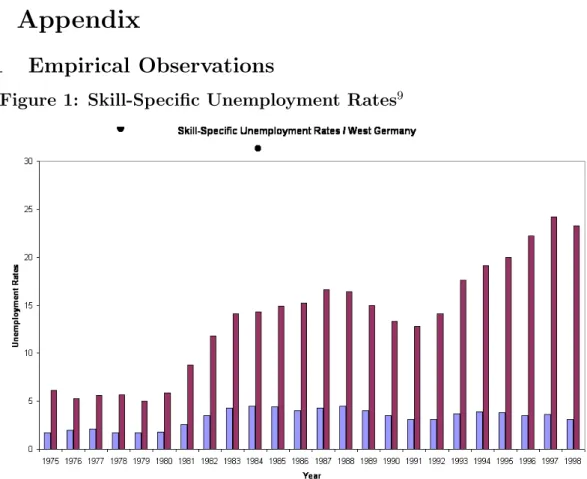
Figure 1: Skill-Specific Unemployment Rates⁹

blue: college degree, red: no formal degree

Table 1: Benefits of Education in the U.S. and West Germany¹⁰

USA

Year UR high educ. UR low educ.

1970 1.1 2.4

1990 2.1 5.3

West Germany

Year UR high educ. UR low educ.

1975 1.2 6.1

1998 3.5 23.3

UR - Unemployment Rate

7.2 Calibration Results

Figure 2: Calibration a. for the job destruction rate χ

9Source: Bundesagentur fuer Arbeit

10Sources: Cuadras-Morato/Mateos-Planas (2006) (USA), Bundesagentur fuer Arbeit (Ger- many)

7.3 Derivations

The representative workerichooses the streams of consumptionC_tⁱ, time in searching sⁱ_t, and investment in education eⁱ_t so as to optimize her utility.

max

cⁱ_t,sⁱ_t,eⁱ_t

E_t

∞

X

t=0

β^t

lnC_tⁱ+φⁱlnhⁱ_t+ (1−φⁱ) ln

1−eⁱ_t−sⁱ_t−Lⁱ_t +λt{Wⁱ(ht)

P_t Lⁱ_t+ b

P_thⁱ_tsⁱ_t+ ε

P_t[1−sⁱ_t−Lⁱ_t]−C_tⁱ− τ P_teⁱ_t} whereLⁱ_t is determined by yesterday’s search.

hⁱ_t+1 = (1−δ)hⁱ_t+eⁱ_t The labor market transition is

Lⁱ_t+1 =

1−χⁱ_t(hⁱ_t)

Lⁱ_t+f_tsⁱ_t The First-Order Conditions are:

FOC ∂/∂C_tⁱ

∂U_tⁱ

∂C_tⁱ =λ_t FOC ∂/∂e_t

∂U_tⁱ

∂lⁱ_t

∂lⁱ_t

∂eⁱ_t−λt

τ

P+β[∂E_tU_t+1ⁱ

∂hⁱ_t+1

∂hⁱ_t+1

∂eⁱ_t +λt+1

b

P_tsⁱ_t+1∂hⁱ_t+1

∂eⁱ_t +λt+1

Lⁱ_t+1 P_t

∂W_tⁱ(ht+1)

∂hⁱ_t+1

∂hⁱ_t+1

∂eⁱ_t ] = 0 U_lt +λ_t τ

Pt

=β[E_tU_ht+1+U_Ct+1 b Pt+1

sⁱ_t+1+U_Ct+1Lⁱ_t+1 Pt+1

∂W_tⁱ(h_t+1)

∂hⁱ_t+1 ] (21) FOC∂/∂sⁱ_t

0 = −U_lt +λ_t

bhⁱ_t− ε Pt

−f_tβU_lt+1+βλ_t+1Wⁱ(h_t+1) Pt+1

f_t−f_tβλ_t+1 ε Pt+1

U_lt +f_tβE_tU_lt+1 =U_Ct

bhⁱ_t− ε P_t

+βf_tE_tU_Ct+1[Wⁱ(h_t+1) P_t+1 − ε

P_t+1] (22) 7.3.1 Short Run Equilibrium

The bargaining aims at maximizing the common bargaining function:

maxw (1−η) ln(V_tⁱ−V) +ηlnZ_t^WN_tⁱ, (23) whereV = 0, and the steady state

Vⁱ = 1 1−(1−δ)β

F(hⁱ, Nⁱ)Pⁱ−

Wⁱ(hⁱ)Nⁱ+κⁱχ(hⁱ)NⁱP q

.

From the workers’ view, the difference of being employed and unemployed is Z_tⁱ =W_tⁱ(hⁱ_t)−bhⁱ_tP_t+

f_tⁱ−χ(hⁱ_t)

βE_tZ_t+1ⁱ (24) whereas in the steady state,

Zⁱ = Wⁱ(hⁱ)−bhⁱP

1−β[fⁱ−χ(hⁱ)]. (25)

Derived from equation (23), the First-Order Condition on wage is:

(1−η) −Nⁱ

F(hⁱ, Nⁱ)Pⁱ−

WⁱNⁱ+κ^{i χ(hi}_q^{)N P} +η N_tⁱ

(Wⁱ−hⁱbP)N_tⁱ = 0 and the aggregate wage is

Wⁱ(hⁱ)Nⁱ = (1−η)hⁱbP Nⁱ+ηF(hⁱ, Nⁱ)Pⁱ−ηκⁱχ(hⁱ)NⁱP

q (26)

Taking derivative according to labor input yields

∂WⁱNⁱ

∂Nⁱ = (1−η)hⁱbP +η∂Y Pⁱ

∂Nⁱ −ηκⁱχ(hⁱ)P q

∂Y Pⁱ

∂Nⁱ − ∂WⁱNⁱ

∂Nⁱ = ∂Y Pⁱ

∂Nⁱ (1−η)−(1−η)hⁱbP +ηκⁱχ(hⁱ)P q The firm’s Euler equation in steady state is:

κⁱP

qⁱ = β(1−δ)

1−β(1−δ) [1−χ(hⁱ)]

∂YⁱPⁱ

∂Nⁱ −∂Wⁱ(hⁱ)Nⁱ

∂Nⁱ

Apparently,

∂YⁱPⁱ

∂Nⁱ = 1−β(1−δ) [1−χ(hⁱ)]

β(1−δ)(1−η)

κⁱP

qⁱ +hⁱbP − ηχ(hⁱ)P (1−η)

κⁱ q

Besides, from the demand function we have:

∂YⁱPⁱ

∂Nⁱ =P I^1σ ∂Yⁱ

∂Nⁱ

Yⁱ + (nⁱ −1)Yⁱ⁻¹_σ⁻¹

(nⁱ−1)Yⁱ+ (1− 1 σ)Yⁱ

therefore,

1−β(1−δ) [1−χ(hⁱ)]

β(1−δ)(1−η)

κⁱP

qⁱ +hⁱbP − ηχ(hⁱ)P (1−η)

κⁱ q

= P I^1σαhⁱ hⁱNⁱα−1h

hⁱNⁱα

+ (nⁱ−1)Yⁱ i−¹

σ−1

(nⁱ−1)Yⁱ+ (1− 1

σ) hⁱNⁱα This equation implicitly gives us the labor input for each firm level, which in turn determines the output of this firm. Since this is the result from the bargaining