An approach to build an event set of European windstorms based on ECMWF EPS

(1)

www.nat-hazards-earth-syst-sci.net/16/255/2016/

doi:10.5194/nhess-16-255-2016

An approach to build an event set of European windstorms based on ECMWF EPS

R. Osinski^2,1, P. Lorenz^3,1, T. Kruschke^4,1, M. Voigt^5,1, U. Ulbrich¹, G. C. Leckebusch^6,1, E. Faust⁷, T. Hofherr⁷, and D. Majewski⁸

1Institute of Meteorology, Freie Universität Berlin, Berlin, Germany

2CNRM/GAME, Météo-France and CNRS, Toulouse, France

3Meteo Service Weather Research GmbH, Berlin, Germany

4GEOMAR Helmholtz Centre for Ocean Research Kiel, Kiel, Germany

5GFZ German Research Centre for Geosciences, Potsdam, Germany

6School of Geography, Earth and Environmental Sciences, University of Birmingham, Birmingham, UK

7Munich Re, Munich, Germany

8German Weather Service, Offenbach, Germany

Correspondence to: U. Ulbrich (ulbrich@met.fu-berlin.de)

Received: 12 January 2015 – Published in Nat. Hazards Earth Syst. Sci. Discuss.: 9 February 2015 Revised: 19 November 2015 – Accepted: 11 December 2015 – Published: 25 January 2016

Abstract. The properties of European windstorms under present climate conditions are estimated on the basis of sur- face wind forecasts from the European Centre for Medium- Range Weather Forecast (ECMWF) Ensemble Prediction System (EPS). While the EPS is designed to provide forecast information of the range of possible weather developments starting from the observed state of weather, we use its archive in a climatological context. It provides a large number of modifications of observed storm events and includes storms that did not occur in reality. Thus it is possible to create a large sample of storm events, which entirely originate from a physically consistent model, whose ensemble spread represents feasible alternative storm realizations of the covered period. This paper shows that the huge amount of identifiable events in the EPS is applicable to reduce uncertainties in a wide range of fields of research focusing on winter storms.

Windstorms are identified and tracked in this study over their lifetime using an algorithm based on the local exceedance of the 98th percentile of instantaneous 10 m wind speed, which is associated with a storm severity measure. After removing inhomogeneities in the data set arising from major modifications of the operational system, the distributions of storm severity, storm size, and storm duration are computed. The overall principal properties of the homogenized EPS storm data set are in good agreement with storms from the ERA-

Interim data set, making it suitable for climatological investigations of these extreme events. A demonstrated benefit in the climatological context by the EPS is presented. It gives clear evidence of a linear increase of maximum storm intensity and wind field size with storm duration. This relation is not recognizable from a sparse ERA-Interim sample for long-lasting events, as the number of events in the reanalysis is not sufficient to represent these characteristics.

1 Introduction

According to the records of insurance and re-insurance com- panies, windstorms are the most costly natural hazards in Europe (Münchener Rückversicherungs-Gesellschaft, 2011).

Fortunately, the most extreme events occur very rarely, but this makes it difficult to estimate their recurrence periods and other statistical characteristics, which can only be estimated with large error bars assigned to them (cf. Della-Marta et al., 2009). Studies estimating these parameters make use of reanalysis and station data (e.g., Della-Marta et al., 2009 or Hofherr and Kunz, 2010) or climate simulations (e.g., Lecke- busch et al., 2006). Most recently, a catalogue of damaging European windstorms was produced by Roberts et al. (2014), based on the European Centre for Medium-Range Weather

(2)

Forecast (ECMWF) ERA-Interim reanalysis. As one impli- cation of this study, it can be said that the Ensemble Predic- tion System (EPS) provides a reasonable opportunity to en- large such a catalogue substantially. So far, statistical models like the random walk or Markov Chain Monte Carlo models are often used to extend samples for the estimation of the recurrence of severe storm events or extreme wind speed with return periods of over 1000 years (e.g., Dukes and Palutikof, 1995). We use the EPS for the same purpose of extending the sample size with the distinction that all EPS events are fully based on a physical model, which has the big advantage of a good consistency and coverage of the potential storm- related risk. In a statistical sense, observations represent the realized reality. Ensemble forecasts as part of the regular weather forecasts demonstrate that individual weather events could have developed differently, starting from basically the same initial weather conditions. In this sense, observations do not provide information on potential alternative developments that could have been reality with a similar probability.

Studies on the EPS are mainly focused on the quality of the prediction. An example of such a study related to European winter storms can be found in Buizza and Hollingsworth (2002), where the focus lies on the predictability of the heav- ily impacting winter storms of the year 1999. Froude (2006, 2009) has analyzed the predictability of storm tracks and ex- tratropical cyclones using a cyclone-tracking algorithm by Hodges (1994). Froude and Gurney (2010) focused on the application of the EPS for the oil and gas industry. The out- put of the ECMWF EPS in an impact-based study was used for estimating the range of potential storm surge events at the German bight (Koziar and Renner, 2005). The small area investigated in this study is, however, not representative of winter storms in Europe. The current study aims at assessing climatological properties of European winter storms, produced by the operational ECMWF Ensemble Prediction System.

Such an approach requires minimizing the effects from inhomogeneities in the EPS introduced by the regular updates of this operational system. They could potentially produce systematic deviations from observed storms, the latter being represented by the ERA-Interim reanalysis in our study. Beyond these changes, there could be systematic forecast-lead-time- dependent trends in the EPS data set, affecting storm characteristics like severity, duration, or the affected areas. Possible breaks (e.g., between different model cycles), trends (e.g., a model drift), and biases (e.g., different wind speed distributions according to different model resolutions) caused by the EPS inhomogeneities in the detected storm properties must be initially addressed in order to carry out climatological investigations.

The paper aims at demonstrating that it is possible to produce statistics of storms under observed climate conditions based on EPS forecasts, leading to more reliable results than traditional approaches based on reanalysis data. Our aim is a representation of the recent climate, which distinguishes our approach from others based for example on climate projec-

tions. To summarize, our study intends to describe a possibility of producing more reliable storm statistics which are still very close to the observed climate. The final event set is comparable to those which are stochastically generated based on a fixed historical sample, with the distinction that the stochas- tics is replaced by the application of a physical model in our case.

2 Data

Instantaneous 10 m wind speed data at different archiving time steps as mentioned farther below are considered. The area of investigation covers the Atlantic–European region spanning from 40^◦W to 40^◦E and 25 to 80^◦N. For part of the studies in this paper (explicitly mentioned in the respective sections), the entire Northern Hemisphere was used in order to avoid boundary effects. An extended winter season is used from September to May.

2.1 ERA-Interim

An archive of 6-hourly ERA-Interim reanalysis data (Dee et al., 2011) is used. At the time the current study was performed, data before the year 1989 were not available, so the period considered is 1989 to 2010. ERA-Interim uses the 4D- Var assimilation scheme and the Integrated Forecast System (IFS) release Cy31r2 at a horizontal spectral resolution of T_L255. The same system release was operational for the EPS from 12 December 2006 until 5 June 2007, but with horizontal resolution of T_L399 (for details refer to Palmer et al., 2007).

2.2 ECMWF Ensemble Prediction System

This section provides some relevant aspects about the ECMWF EPS. A more detailed description of the EPS can be found in Palmer et al. (1992, 2007) and Molteni et al.

(1996). The Ensemble Prediction System of the ECMWF became operational in December 1992 (see Table 1 for an overview). Initially, 32 perturbed forecast members (based on the method of singular vectors; in the following abbreviated as “pf”) plus one control forecast (not perturbed against the original analysis, but using the EPS model system instead of its deterministic counterpart; in the following abbreviated as “cf”) were produced. The number of perturbed ensemble members was increased to 50 in December 1996. Since Oc- tober 1998, some of the EPS runs have been produced including perturbations in the model physics. With increasing computing power, continuous upgrades of the system lead to improvements in the forecast skill (cf. Palmer et al., 2007).

The horizontal resolution was increased from T63 as fol- lows: T_L159 (December 1996), T_L255 (November 2000), and T_L399 (February 2006) to eventually (not used in this study) T_L639 (January 2010). The resolution of the singular vectors was changed from T21L31 to T42L31 (March 1995),

(3)

T42L40 (October 1999), and eventually T42L62 (Febru- ary 2008) (Palmer et al., 2007). Changes in the data assimilation scheme (Rabier et al., 2000; Mahfouf and Rabier, 2000;

Klinker et al., 2000) from 3D-Var to 4D-Var were introduced in November 1997 (cf. Bouttier and Rabier, 1997). The EPS integration time is 15 days, but after 10 days of forecast the horizontal resolution is decreased. Since March 2003, the system has been initialized twice a day, at 12:00 and 00:00 UTC. In order to take the major changes into account, the data set was split into periods with constant horizontal resolution (Table 1). Data used in this study cover the period until 25 January 2010, thus excluding the latest period with TL639 resolution. Depending on the period, the EPS data are available at 12-, 6-, and 3-hourly temporal resolution. As ERA-Interim is only available at 6-hourly resolution, the EPS data with a 3 h resolution were used in subsets of 6- hourly resolution. For the 12-hourly data, ERA-Interim was also used at this temporal resolution (time steps at 00:00 and 12:00 UTC).

3 Methods

3.1 Identification and characterization of storms at midlatitudes – wind tracking

For the identification and characterization of European winter windstorms, an impact-related wind-tracking algorithm is used. It was introduced by Leckebusch et al. (2008) and has been further developed since then. An overview of the actual scheme is provided by Kruschke (2015). It identifies grid points belonging to windstorms by searching for spatial clusters of grid points (extending over an area of at least 1.6×10⁵km²) where the local 98th percentile of wind speed is exceeded. The choice of the 98th percentile is motivated by the relevance of this threshold for storm damages (Klawa and Ulbrich, 2003). The identified clusters are connected to a track using a nearest-neighbor criterion. The maximum distance allowed to connect two clusters to a windstorm track is limited by an assumed maximum wind field propagation velocity of 120 km h⁻¹. In the present study a minimum lifetime of 24 h of an identified windstorm must be fulfilled, equivalent to three archived time steps for the 12 h temporal resolution and five time steps for 6 h resolution periods (Table 1). By summing the cube of the 98th-percentile exceedances belonging to a track, an objective storm severity measure is determined. This measure, called the storm severity index (SSI), is calculated for each storm over all time stepstand grid pointskaffected by exceedances of the 98th percentile assigned to a storm. It is meant to character- ize the severity of storms, taking intensity, size, and duration of the storms into account, as is shown in Eq. (1):

SSI=

T

X

t K

X

k

"

max

1, v_k,t v_perc,k

−1 3

·Ak

#

. (1)

vk,t is the wind velocity in grid cell k at time instance t, vperc,k the 98th percentile in grid cell k, and Ak the area of grid cellk. The SSI values are normalized to a grid cell of unit size. This is done using the grid cell area A_k to reduce the resolution dependence when applying different models and to eliminate a latitude dependence. A resolution dependence can still remain, as models of different resolutions can produce different wind speed distributions. This will be discussed in the following section. The algorithm was originally developed for the application with reanalysis and climate data. The medium-range ensemble EPS consists of single forecasts from which we use the first 10 days. For each day up to twice a day (12:00 and 00:00 UTC initializations) 50 perturbed forecasts and an additional control forecast were produced and archived. The algorithm is applied on each individual forecast. This means that, when combining the members and forecasts with different lead times, a single day is represented by up to (50pf+1cf)×2 initializations×10 days=1020 equivalent days. To avoid boundary effects at the beginning and end of the forecasts, the period had to be reduced to be able to generate representative samples. We restricted our sample to EPS runs initialized at 12:00 UTC with storms starting inside a window of 6 forecast days (to be discussed in Sect. 4.3). This results in an enlargement of the sample deducible from reanalysis by a factor of 300 using perturbed forecasts.

3.2 Homogenization of the EPS

The improvements introduced into the operational EPS system mentioned above will affect the results of the tracking procedure in different ways, but a main impact is due to the changes in spatial and temporal resolution. Hence, we subdi- vide the data into subperiods of the same spatiotemporal resolution and apply a two-step procedure to homogenize windstorm identification and SSI calculation across these subperiods: first, the 98 % quantiles of each subperiod are scaled towards a common basis, using the ERA-Interim data set as a reference. We call this the “climatological scaling” of the threshold used for windstorm identification (see Sect. 3.2.1).

Second, a quantile–quantile mapping approach (cf. Boé et al., 2007; Maraun, 2013) is used for exceedances of the 98th percentile to provide matching shapes of the upper tail of the wind speed distribution, which is a requirement of SSI calcu- lations, homogenous across all subperiods. This second step is called “scaling of exceedance” in the context of this study (see Sect. 3.2.2).

3.2.1 Climatological scaling

Subdividing the EPS data set into periods which are homoge- neous in terms of the horizontal resolution of the model system (see Table 1) reflects the finding that different resolutions of the EPS system produce different wind speed biases and, as a consequence, biases in SSIs, storm duration, and size.

(4)

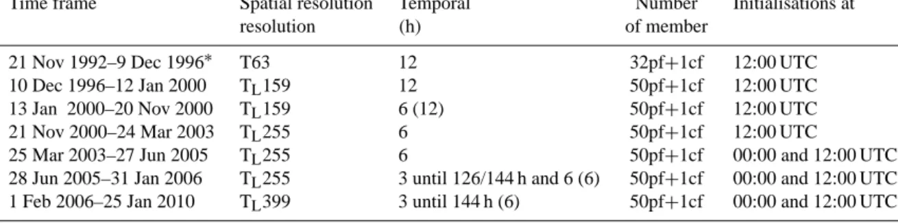
Table 1. Overview of general characteristics of the EPS (used temporal resolution) pf: perturbed forecast; cf: control forecast.

Time frame Spatial resolution Temporal Number Initialisations at

resolution (h) of member

21 Nov 1992–9 Dec 1996^∗ T63 12 32pf+1cf 12:00 UTC

10 Dec 1996–12 Jan 2000 T_L159 12 50pf+1cf 12:00 UTC

13 Jan 2000–20 Nov 2000 T_L159 6 (12) 50pf+1cf 12:00 UTC

21 Nov 2000–24 Mar 2003 T_L255 6 50pf+1cf 12:00 UTC

25 Mar 2003–27 Jun 2005 T_L255 6 50pf+1cf 00:00 and 12:00 UTC

28 Jun 2005–31 Jan 2006 T_L255 3 until 126/144 h and 6 (6) 50pf+1cf 00:00 and 12:00 UTC 1 Feb 2006–25 Jan 2010 T_L399 3 until 144 h (6) 50pf+1cf 00:00 and 12:00 UTC

∗Before January 1994 only three forecasts per week available, major change on the system with introduction of the IFS in March 1994 and the introduction of IFS cycle 12r1, which led to a significant reduction in the model bias of 10m wind speed

(http://www.ecmwf.int/en/forecasts/documentation-and-support/evolution-ifs/cycle-archived/1994-summary-changes).

ERA-Interim clim ERA-Interim subEPS EPS

EPS climERA-Interim

Figure 1. 98th percentile as average over all land boxes (accord- ing to land-sea masks of the data set) in the domain from 40^◦W to 40^◦E and 25 to 80^◦N for different EPS subperiods with corresponding 98th ERA-Interim land box percentile: climatological ERA-Interim percentile based on ERA-Interim for period 1989–

2010 (ERA-Interim clim), ERA-Interim percentiles for the periods of the corresponding EPS periods (ERA-Interim sub_EPS), percentiles of raw EPS data (EPS), and climatologically adjusted EPS percentiles (EPS climERA-Interim).

A model with a coarse resolution represents an average of a larger grid cell area than a model with a fine resolution. The finer the model resolution, the better the orographic effects that can be captured. This influences the wind speed distributions, but differences in wind speed characteristics for the periods considered can also originate from climate variability.

The latter becomes evident when the ERA-Interim data are used for estimating this threshold for the whole period and for the same subperiods: Fig. 1 shows 98th ERA-Interim percentiles using all land grid points in the Atlantic–European area chosen. Land grid points are shown, as the major interest is related to storm damages over land, but the method is applied on all individual cells of the entire grid. The estimates for the four subperiods vary from the percentile computed for the complete period 1989 to 2010. The percentiles of the EPS versions with coarser horizontal resolution are found to be lower than those with higher resolution. The effect from T_L159 to T_L255 is much stronger than from T_L255 to T_L399.

Note that for this intercomparison an interpolation towards the ERA-Interim grid had to be performed. The correction

98 98.2 98.4 98.6 98.8 99 99.2 99.4 99.6 99.8

0 10 20 30 40 50

Percentile

Relative exceedance of 98th percentile [%]

T63 T L159 TL255 TL399

Figure 2. Visualization of tail differences in the wind speed dis- tribution of the four subperiods (see Table 1) of the EPS. Shown:

relative exceedance of 98th EPS percentile as land average. Internal climate variability of the disjunct periods is excluded by utilization of the climatological scaling (for details see text).

factor for the 98 % quantile of each grid cell is computed taking the factor due to climate variation (as estimated from ERA-Interim) into account.

3.2.2 Scaling of exceedance

After climatological scaling of the identification threshold, the wind speeds exceeding this 98th percentile still differ between the subperiods, as shown in Fig. 2. The presented differences in the tail seem to be very small, but as the cubic of these values is used and summed over a larger quantity of grid cells for the SSI calculation, cf. Eq. (1), they are impacting the results. For this reason, a quantile–quantile mapping is used. It is a standard method used for a bias correction; see, e.g., Maraun (2013). The method chosen estimates empirically percentiles in equidistant steps (0.1 %) for both EPS and ERA-Interim. A wind value in the EPS, which cor- responds to the ith percentile of the EPS wind speed distribution, is corrected in the way that it has afterwards the value of theith percentile of the ERA-Interim wind distribution. After both climatological scaling and quantile–quantile mapping, the ERA-Interim 98th percentile and the exceeding wind speeds mapped on the ERA-Interim distribution can be

(5)

0 24 48 72 96 120 144 168 192 216 240 5

6 7 8 9 10

T63 Land

12UTC

0 24 48 72 96 120 144 168 192 216 240 13

13.5 14 14.5 15 15.5 16

T63 Sea

12UTC

0 24 48 72 96 120 144 168 192 216 240 7

8 9 10 11

TL159 Land

12UTC

0 24 48 72 96 120 144 168 192 216 240 16

16.5 17 17.5 18

TL159 Sea

12UTC

0 24 48 72 96 120 144 168 192 216 240 7

8 9 10 11

TL255 Land

12UTC

0 24 48 72 96 120 144 168 192 216 240 16

16.5 17 17.5 18

TL255 Sea

12UTC

0 24 48 72 96 120 144 168 192 216 240 7

8 9 10 11

TL399 Land

00UTC 12UTC

0 24 48 72 96 120 144 168 192 216 240 16

16.5 17 17.5 18

TL399 Sea

00UTC 12UTC

(a)

(b)

(c)

(d)

(e)

(f)

(g)

(h)

[h]

[m/s]

Figure 3. Average of 98th percentile (m s⁻¹) for different forecast lead times (right axis, h after initialization): for T63 12-hourly (a, e), T_L159 12-hourly (b, f), T_L255 6-hourly (c, g), and T_L399 6-hourly (d, h). (a)–(d) for land grid boxes, (e)–(h) for sea grid boxes.

used for the SSI calculation in every subperiod. A quantile–

quantile mapping for the different periods without previous climatological scaling is not suitable, as it would completely remove the (real) climate variations.

4 EPS storm validation

4.1 Spin-up effects, threshold, and diurnal cycle Even though spin-up effects in numerical simulations are well known, their magnitudes in the ECMWF EPS have not been a major issue in the scientific literature. An exception is the report by Lamquin et al. (2009) focusing on humidity in the upper troposphere. Results of an analysis on systematic variations of 98 % quantiles of wind speed are given in Fig. 3 for the T63, TL159, TL255, and TL399 resolutions. Average values over all land and all sea boxes in the area considered have been computed for archiving steps of the forecasts. For both land and sea grid points a small initialization effect in the first 6 to 12 h of the forecasts becomes visible. The percentile value in the T_L159 resolution over land, for example, is about 0.5 m s⁻¹higher during the first one to two archiving time steps than subsequently. Over sea, there seems to be an effect with opposite signature (lower initial values) in the first 12 to 18 forecast hours. The data for T_L399 over sea show the same initialization effect. The dominant feature in Fig. 3 is, however, a diurnal cycle with an amplitude of about 1 m s⁻¹ over land. Maxima occur at the forecast time steps valid at noon (12:00 UTC). Note that a corresponding cycle

is also found in the ERA-Interim data, with about the same amplitude (not shown). Conventional observations confirm that the daily cycle in the 10 m wind speed over land is a realistic feature (Lapworth, 2008, 2012). The EPS with T_L255 is characterized by an interfering daily periodicity and an 18 h periodicity. As the daily cycle is small over sea, the 18 h periodicity is clearly visible in Fig. 3g. The irregular behavior of the EPS with TL255 resolution is apparently related to the stochastic perturbations of the model physics used during the respective period (A. Beljaars, personal communi- cation, November 2012) as the unperturbed control forecast produces a regular daily cycle (figure not shown). A more thorough investigation of the 18 h cycle is beyond the scope of the present paper. We have not attempted to remove it from the investigation, but in comparing the windstorm statistics for this EPS resolution with the other periods we found no evidence for a systematic effect.

4.2 Modifications of observed storms in the EPS: storm

“Emma”

Different EPS members started at different lead times will produce modifications of observed storm events in terms of their genesis time, track, and intensity. Before considering the respective statistics for the whole time series, we con- sider the storm event named¹Emma (28 February 2008) as an example in more detail. At a lead time of 6 h, all of the

1Names are given by the Institute of Meteorology of the Freie Universität Berlin.

(6)

1 0 2 0 3 0 4 0 5 0 0

2 0 4 0 6 0 8 0

SSI

1 0 2 0 3 0 4 0 5 0

0 2 0 4 0 6 0 8 0

Ensemble member

SSI

EPS

ERA -Interim-Interim ERA-Interim (a) EPS

(b)

Figure 4. SSIs for representations of the storm Emma (28 Febru- ary 2008, 18:00 UTC, detected in ERA-Interim) in 50 EPS mem- bers: (a) 6 h lead time, initialized 28 February 2008 at 12:00 UTC and (b) 90 h lead time, initialized 25 February 2008 at 00:00 UTC.

10 20 30 40 50

0 0.5 1 1.5

2x 10⁶

Ensemble member Average Clustersize [km2]

10 20 30 40 50

0 20 40 60 80 100

Ensemble member

Duration [h]

EPS ERA -Interim

(a) (b)

Figure 5. Representation of the storm Emma (28 February 2008, 18:00 UTC, detected in ERA-Interim) in 50 EPS members ini- tialized 28 February 2008 at 12:00 UTC. (a) Average cluster size (km²), (b) duration (h).

50 EPS runs produce a storm fulfilling our criteria that can be assigned to the observed one (Fig. 4a). The majority of the simulated events are weaker than the intensity computed from ERA-Interim, but for 12 members the simulated storm is stronger than observed. At a lead time of 90 h, taken as a second example (Fig. 4b), in several runs no storm is found.

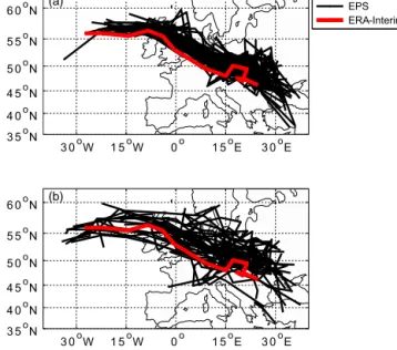
One member, however, produces a storm of about double the observational SSI. The variations in SSI originate from variations in the intensity at individual grid points, in area and in storm lifetime, as depicted in Fig. 5 for the 6 h lead time. The track of Emma in ERA-Interim and in the individual EPS members (Fig. 6) is found by identifying a storm core from the weighted local SSI contributions of all storm grid points at a time step, and connecting the centers from different time steps (Leckebusch et al., 2008). While in many other cases the observed storm is found close to the center of the EPS

3 0ôW 1 5ôW 0ô 1 5ôE 3 0ôE 3 5ôN

4 0ôN 4 5ôN 5 0ôN 5 5ôN 6 0 Nô

ERA^¡ INT EPS

3 0ôW 1 5ôW 0ô 1 5ôE 3 0ôE 3 5ôN

4 0ôN 4 5ôN 5 0ôN 5 5ôN 6 0ôN

ERA-Interim^¡ (a) EPS

(b)

Figure 6. Tracks for representations of the storm Emma (28 Febru- ary 2008, 18:00 UTC, detected in ERA-Interim) in 50 EPS members initialized on (a) 28 February 2008 at 12:00 UTC and 50 members initialized on (b) 25 February 2008 at 00:00 UTC.

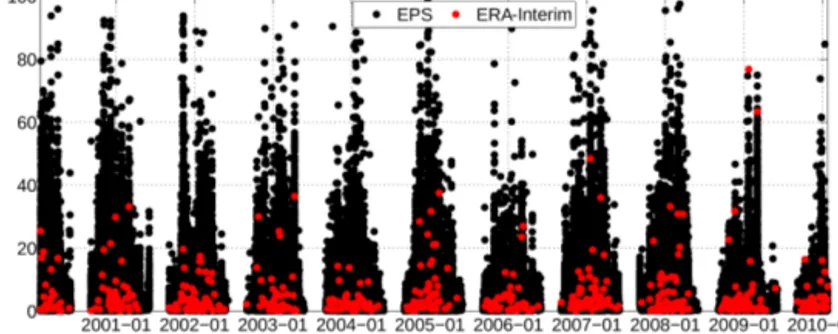
ensemble member storms, all EPS tracks of Emma at this lead time are located northward of the ERA-Interim storm (Fig. 6a). For the 90 h lead time (Fig. 6b), the spread between the modified Emma tracks is larger. A notable feature of Emma is the fact that the observed Emma tends to be at the border of the EPS ensemble also for the long lead time. This example demonstrates that extreme EPS events can be feasible representations, but the northward shift is not systematic in the EPS. SSI values for all events detected in ERA-Interim and the EPS (starting inside a 6-day window; see Sect. 4.3) over the period 2001 to 2010 are shown in Fig. 7. Over the entire period, the range of SSI in the EPS is much larger than in ERA-Interim. A larger range of SSI values was expected, as the EPS can include forecasts with slightly higher wind ve- locities. The definition of the SSI, using cubic exceedances, enlarges the range of values. As the motivation for the SSI definition is damage potential, the additional events help to better estimate potential storm risks for Europe, in particular with respect to the occurrence of the most extreme storms.

4.3 Comparison of storm properties in the EPS and ERA-Interim

In order to compare the entire ensemble of storms in the EPS with those detected in the ERA-Interim data set, events not entirely captured in a forecast must be excluded. They would erroneously be taken as short(er)-lived storm events.

This situation may be present if a storm is detected at the initialization time. In this case, it may have existed before but could not be completely tracked on the basis of the driving data. Removing all storms existing at the start of the fore-

(7)

Figure 7. SSIs for all storms in the period 13 January 2000 (10 m wind available at 6-hourly resolution for the EPS) to 25 January 2010 for ERA-Interim and for the EPS with initializations at 12:00 UTC. The months June, July, and August are excluded.

Table 2. Average storm properties of EPS (ERA-Interim).

Resolution No. per year Size[10⁶km²] Duration[h] T63^∗(12-hourly) 50.9 (54.0) 0.70 (0.65) 41.2 (43.8) T_L159 (12-hourly) 45.9 (49.3) 0.75 (0.79) 49.2 (50.4) T_L255 (6-hourly) 47.6 (45.0) 0.71 (0.76) 41.4 (42.0) TL399 (6-hourly) 47.9 (50.5) 0.74 (0.74) 42.0 (42.6)

∗Based on data from 1 January 1995 to 9 December 1996.

cast, however, allows the full range of storm durations to en- ter the statistics without a bias. A similar kind of problem would occur with storms existing at the end of the 10-day forecast time. Here, the same solution cannot be applied as it would prefer short-duration storms for genesis occurring rather late in the forecast period. We decided to restrict the evaluated storms to those generated a maximum of 6 days after forecast initialization, leaving 4 days as a maximum duration. There is still a problem with storms lasting 4 days or longer. According to ERA-Interim, only 0.8 % of storms are this long-lasting, and only some of them (namely, those generated at one of the time steps just before the 6-day limit) are affected. We expect the impact on the results to be small.

Also, the choice of 6 days is motivated in the fact that it leads to an equal frequency of evaluated time steps at 0, 6, 12, and 18 h forecast time, thus ameliorating the effects of the 18 h periodicity in intensities mentioned earlier.

Initializations at 00:00 UTC are only available after March 2003, as is shown in Table 1. We wanted to be sure to avoid an overrepresentation of the period 2003 to 2010 in the statistics and thus use only the 12:00 UTC initializations. Nevertheless we looked into the forecasts initialized at 00:00 UTC and found no systematic difference compared with the runs starting at 12:00 UTC. Using the 6-day window, one initialization per day, and 50 perturbed forecasts for the period 2000 to 2010 yields a storm sample 300 times larger than available from reanalysis data for the same period.

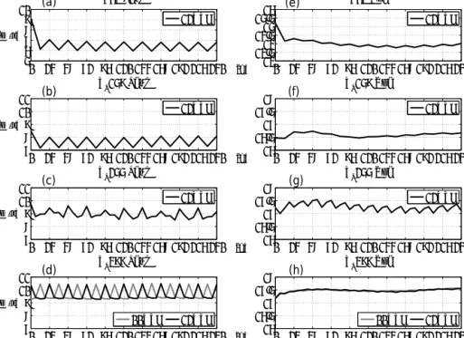
Storm properties in the EPS compared to ERA-Interim The average number, size, and duration of storm events per year found in the four different time periods characterized by the specific EPS resolutions are given in Table 2, both for the EPS and ERA-Interim. The number of events in the EPS is the ensemble average over all available ensemble members, initializations per day, and over the forecast length limited to storms lying inside the described 6-day window (cf. Sect. 4.3). This number can thus be directly compared to the ERA-Interim values given in the same table. The respective values are similar between the two data sets, meaning that the storm properties in the EPS ensemble average are in good agreement with ERA-Interim. In order to compare the severity distributions of the EPS and ERA-Interim events, seven severity classes were formed making sure that there is a reasonable number of events in each of the classes to permit statistical tests. Subperiods with constant horizontal resolution of the EPS are again distinguished. Note that the SSI values calculated from data with 12-hourly resolutions (T63 and TL159) are expected to be lower than those from 6-hourly resolutions (T_L255 and T_L399) (Fig. 8) due to the additional time steps included for the latter. It can be seen how the results of the wind tracking differ for the EPS without using any scaling technique, using only the climatological scaling, the scaling of exceedance, or both together. When both scaling techniques are used together, the severity distributions of the EPS and ERA-Interim are comparable for all subperiods except for EPS T63. For the latter, the scaling corrects for an overestimation of severity, resulting in a good agreement in the highest four severity classes. The larger number of weak events has its origin in model biases of 10 m wind speed²during the early years (1992 to 1994) of the data period of the T63 EPS. As it is difficult to evaluate the benefit of the scaling techniques visually, a normal distribution was fitted to the logarithm of the SSI. The Anderson–Darling test (Thode, 2002) indicates that the logarithm of the SSI is normally dis-

2http://www.ecmwf.int/en/forecasts/

documentation-and-support/evolution-ifs/cycle-archived/

1994-summary-changes

(8)

0.5 1.5 3.5 6.5 10.5 15.5 21.5 max 0

5 10 15 20 25 30 35

SSI

No.eventsperyear Era Interim

EPS (T63) EPS (T63) clim EPS (T63) exceed EPS (T63) clim+exceed

0.5 1.5 3.5 6.5 10.5 15.5 21.5 max

0 5 10 15 20 25 30 35

SSI

EPS (T^L159) EPS (T^L159) clim EPS (TL159) exceed EPS (TL159) clim+exceed

0.5 1.5 3.5 6.5 10.5 15.5 21.5 max

0 5 10 15 20 25 30 35

SSI

EPS (TL255) EPS (TL255) clim EPS (TL255) exceed EPS (T^L255) clim+exceed

0.5 1.5 3.5 6.5 10.5 15.5 21.5 max

0 5 10 15 20 25 30 35

SSI

EPS (TL399) EPS (TL399) clim EPS (TL399) exceed EPS (T^L399) clim+exceed

(a) (b)

(d) (c)

Figure 8. No. of storm events per year subdivided according to the severity, for the four individual subperiods with constant horizontal resolution: (a) T63, (b) T_L159, (c) T_L255, and (d) T_L399 of the EPS (T63 and T_L159 at 12-hourly resolution for EPS and ERA-Interim).

First bar is for ERA-Interim, the other for the EPS (bars from left to right): second – EPS raw data; third – processed by climatological scaling; fourth – processed by scaling of exceedance; and fifth – applying both scaling techniques on the data.

−4 −2 0 2 4 6

0.000.050.100.150.200.250.300.35

log(SSI)

Density

Fit ERA-Interim Fit EPS Fit EPS clim Fit EPS exceed Fit EPS clim+exceed

−4 −2 0 2 4 6

0.000.050.100.150.200.250.300.35

log(SSI)

Density

Fit ERA-Interim Fit EPS Fit EPS clim Fit EPS exceed Fit EPS clim+exceed

(a) (b)

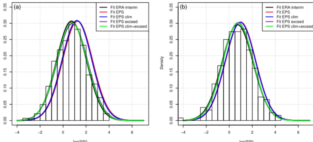
Figure 9. Fit of normal distributions to logarithm of SSI for (a) EPS in TL255 and (b) EPS in TL399 without scaling techniques, with climatological scaling, with exceedance scaling, and with both scaling techniques together. Raw EPS data and climatologically scaled data are similar and differ more greatly from the observation than using the exceedance scaling or both together.

tributed. The benefit from the scaling techniques is illustrated in Fig. 9. Looking for the raw EPS data at T_L399 resolution, one sees that they concur better with ERA-Interim than the data in T_L255. The effect of the climatological scaling is relatively small. Using both scaling techniques together, the distributions between the EPS and ERA-Interim look very similar. The fit parameters are shown in Table 3. Fit parameters were estimated using maximum likelihood. The exact standard errors of the parameters are very small in the EPS case due to its very large sample. The mean and standard de- viation lies in between the error resulting from ERA-Interim.

This means that the EPS ensemble mean represents well the storm climate which can be found in ERA-Interim. Storm representations in the EPS and ERA-Interim with comparable SSI values show, on average, comparable storm duration as well as the storm size (not shown).

5 Spatiotemporal EPS storm properties 5.1 Pure and modified EPS storms

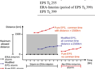
Most considerations in this paper are based on the assump- tion that the EPS produces modifications of storms in the real world (subsequently called “modified EPS storms”), or, for some ensemble members, low wind speeds and thus no storm at all. However, the EPS can produce storm events that have no real-world counterpart. As for statistical investigations independent and identically distributed (iid) random variables are necessary; such pure events are particularly interesting, because they can increase the sample of independent events.

Figure 10 shows a sketch of the definition of pure and modified storms in this study. To identify pure EPS storm events, events are sought for which no simultaneous counterpart can

(9)

Table 3. Parameters and their errors of fitted normal distribution to logarithm of SSI for the EPS using both scaling techniques together and ERA-Interim.

Model Mean SD Error mean Error SD

ERA-Interim (period of EPS T_L255) 0.73 1.30 0.077 0.055

EPS T_L255 0.77 1.32 0.003 0.002

ERA-Interim (period of EPS T_L399) 0.72 1.35 0.086 0.061

EPS TL399 0.76 1.33 0.005 0.004

0 1500 Distance [km]

Modified EPS, all common time distance ≤1500km

Time Storm in ERA-Interim [6h]

Maximum allowed distance

Pure EPS no common time

No ERA-Interim Pure EPS, common time with distance > 1500km

ERA-Interim Modified EPS storm

Pure EPS storm storm

storm

Figure 10. Sketch of definition for pure and modified EPS storms.

be found in ERA-Interim. We also regard events as pure if there is a spatial distance of more than 1500 km between con- temporaneous events, as this is a typical synoptic scale of the investigated phenomena.

5.2 EPS storms during the forecast time

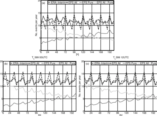
Using the aforementioned method to separate pure and modified storms, it can be assumed that close to the initialization time almost only modified storms can be found in the EPS (Fig. 11). All ensemble members are likely to produce the storm that actually occurred, even if properties like size and duration as well as severity vary between the different realizations. For long lead times, however, there is an increased number of pure EPS storms (grey lines in Fig. 11). The example of the storm Emma illustrates that for longer lead times a number of ensemble members do not show the storm at all, and a larger variability can be found in the intensities. Note that the average number of all storms in the EPS is nearly constant over the forecast time in spite of the small variation in the percentile values (Fig. 3) over forecast time. This number is similar to its ERA-Interim counterpart, supporting our approach to use the individual period’s own percentile for storm identification. A diurnal variation in the number of storms related to the diurnal variation in the 98th percentiles (Fig. 3) is reflected in Fig. 11. As the percentile values used for the wind tracking are based on all data, their values lie between the minimum and maximum value of the 6-hourly or 12-hourly resolution. As at 12:00 UTC the 98th-percentile value is above the 98th percentile of the entire data set, the probability of an exceedance at this time of the day is larger than for the other times. For this reason the number of both

first and final storm track detections is larger at 12:00 UTC than for the other times.

5.3 Spatial distribution of storms

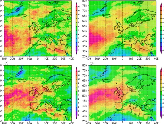
In order to investigate whether there is a difference in the spatial distribution of European winter storms between ERA- Interim and the EPS, the effect of each grid cell by all detected storms per EPS subperiod is computed. The footprint (region of grid cells which is affected by a storm) of each detected storm is analyzed, and for each grid cell the number of footprints affecting this particular grid cell is counted.

Figure 12 shows the results, and for comparability the area effects for ERA-Interim are calculated for the same time frames as the EPS subperiods. The results with the ERA- Interim and EPS T_L255 resolutions have identical grid points and are thus comparable without interpolation. For the comparison for the EPS with T_L399 resolution, the result for ERA-Interim was interpolated to this resolution. For this specific analysis, the entire Northern Hemisphere was used for the tracking to avoid boundary effects caused by a limitation of the area. The basic distribution of the effects is similar in ERA-Interim and the EPS. The lower number (300 times;

EPS with 50 members lasting over 6 days) of events available in the observational data causes a much noisier distribution than what is obtained from the EPS. There are local maxima in ERA-Interim for example over north Africa and the Mediterranean which the forecast model is not able to repro- duce.

5.4 Modified vs. pure EPS storms

The interest in pure EPS storms originates from the wish to find events that are independent of modifications of ERA- Interim storms. Using the same procedure as in the section before to determine the spatial effects, but only for footprints of pure EPS storms, defined after the method explained in Fig. 10, the results are shown in Fig. 13 for the EPS with T_L255. Over the Atlantic the number for the pure EPS storms is lower than over north Africa and eastern Europe. The major pathway of the storm systems is not so strongly affected by pure EPS storms as the regions where storms appear less frequently. The absolute number of pure events can be seen by combining Fig. 12 with Fig. 13. Then we have about 1 pure event over the Atlantic and about 1.5 to 2 over central

(10)

6 24 48 72 96 120 144 168 192 0

5 10 15 20

[h]

No.eventsperyear

T_L255 12UTC

ERA−Interim EPS All EPS Pure EPS All - Pure

6 24 48 72 96 120 144 168 192

0 5 10 15 20

[h]

No.eventsperyear

T_L399 12UTC

ERA−Interim EPS All EPS Pure EPS All - Pure

6 24 48 72 96 120 144 168 192

0 5 10 15 20

[h]

No.eventsperyear

T_L399 00UTC

ERA−Interim EPS All EPS Pure EPS All - Pure (a)

(b) (c)

Figure 11. Temporal evolution of the number of first storm detections during the integration time (h) after initialization (a) T_L255 – 12:00 UTC; (b) T_L399 – 00:00 UTC; and (c) T_L399 – 12:00 UTC. Values for ERA-Interim at 00:00, 06:00, 12:00, and 18:00 UTC are repeated.

Europe. This has the consequence that the use of pure EPS storms as a supplemental amount of events for increasing an independent sample of modified storms leads to a bias in the spatial distribution of storms. Using the presented method, the dependency between events to create an iid sample is defined by a comparison to ERA-Interim. Another feasible approach is to use a matching criterion in between all of the EPS events or a bootstrap-like sampling of alternative realizations of the past. Such approaches using the ECMWF EPS were successfully applied for estimations of return periods of European winter storms by Osinski (2015).

5.5 Storm intensity vs. duration

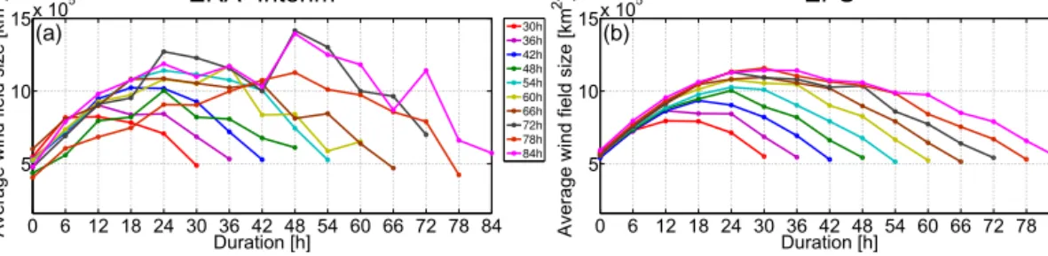
A benefit of storm statistics based on the EPS instead of reanalysis is the larger number of storms available for statistical studies of typical midlatitude storms. Figure 14 shows a clear correlation between the storm duration and the maximum wind field size, which is the maximum of the area of exceedance of the 98th percentile that is assigned to the storm at each particular time step. For storms with durations of up to 54 h, ERA-Interim shows a comparable picture to the EPS.

This can be explained by the fact that the number of observed storms of this timescale is large enough to provide reliable statistics. The EPS indicates that the average growth rate of storms is independent of their duration, while the duration

determines the maximum size of the wind field. For long- lasting events there seems to be an asymmetry between the growth and the decline, where the growth seems to be faster than the decline. With respect to storm severity, a similar in- terdependence is found (Fig. 15). Again, the intensification rate of storms on average is nearly independent of storm duration.

6 Conclusions

Atlantic–European windstorms were identified in the archived data set of the ECMWF Ensemble Prediction Sys- tem forecasts in the period December 1992 to January 2010.

The identification of potentially damaging windstorms was based on the excess over the local 98th percentile of wind speeds (Leckebusch et al., 2008; Kruschke, 2015), only taking into account events which have a minimum area at a single archived time step and a minimum duration of 24 h (with fulfillment of the minimum area criterion in each of them).

The fact that the operational EPS changed its characteristics during the data period led to changes in the value of the 98th percentile of wind speed. Hence a homogenization procedure was applied to four subperiods characterized by different spatial resolutions of the system. Temporal variation of the percentile due to climatic variations and variations with

(11)

(a)

(b)

(c)

(d)

Figure 12. Accumulated yearly number of detected storms (sum of footprints per year) for time frame of the EPS resolution T_L255 (a, c) and T_L399 (b, d), ERA-Interim (a, b), and EPS (c, d) normalized by ensemble size by dividing by 50 members and 6 forecast days.

Figure 13. Percentage of number of EPS storms affecting the grid cell and being pure in the EPS with T_L255 initialized at 12:00 UTC.

respect to the cubic excess over the percentile (assumed to be model version specific) were taken into account. A diurnal cycle in the 98th percentile of the 10 m wind speed was observed in the EPS, which is also present in ERA- Interim. These diurnal variations comprise a systematically higher value of the threshold percentile for 12:00 UTC only, which is about 1 m s⁻¹ larger than the respective values at the other 6 hourly time steps. This effect also leads to a diurnal variation in the number of storm initiations and ends,

as detected by the here-applied storm identification scheme.

Averaged over a large number of storms, this diurnal variation can be seen in the severity at different times of day. This behavior is, however, partly hidden in the EPS with TL255 resolution, as these forecasts additionally exhibit an 18 h periodicity in the threshold for individual time steps presum- ably assigned to the specific stochastical perturbations im- posed in the ensemble-generating process during the respective period. None of these effects had an apparent strong impact on the subsequent evaluations of the EPS as all forecast time steps inside a 6-day window were taken into account.

The overall EPS storm properties were found to be similar to ERA-Interim storm properties. On average the EPS produces the same number of storm days as ERA-Interim. There is no systematic tendency over lead time in the total number of storms. The EPS produces developments of storms which have no observational counterpart. While the principal statistical properties are the same as for modifications of modified representatives of real storms, their share in the total number increases with increasing lead time. They have a spatial distribution of occurrence that is different from the observed and modified storms, with a focus on the Mediterranean and eastern Europe.

As the spatial distribution and the number, the size, and duration of events of same severity are in good agreement with “real” storm events, the EPS can be used to increase the

(12)

0 6 12 18 24 30 36 42 48 54 60 66 72 78 84 5

10 15x 10⁵

Duration [h]

Averagewindfieldsize[km2] ERA Interim

0 6 12 18 24 30 36 42 48 54 60 66 72 78 84 5

10 15x 10⁵

Duration [h]

Averagewindfieldsize[km2] EPS

0 6 12 18 24 30 36 42 48 54 60 66 72 78 84 5

10 15x 10⁵

Duration [h]

Averagewindfieldsize[km2] EPS

0 6 12 18 24 30 36 42 48 54 60 66 72 78 84 5

10 15x 10⁵

Duration [h]

Averagewindfieldsize[km2] ERA Interim

(a) (b)

Figure 14. Wind field size during storm duration for storm duration between 30 and 84 h; (a) for ERA-Interim and (b) for the EPS.

0 6 12 18 24 30 36 42 48 54 60 66 72 78 84 0

0.25 0.5 0.75 1 1.25 1.5

Duration [h]

AverageinstantaniousSSI ERA Interim

0 6 12 18 24 30 36 42 48 54 60 66 72 78 84 0

0.25 0.5 0.75 1 1.25 1.5

Duration [h]

AverageinstantaniousSSI EPS

(a) (b)

Figure 15. Storm severity during storm duration for storm duration between 30 and 84 h; (a) for ERA-Interim and (b) for the EPS.

sample size for European winter storm studies by a factor up to the number of ensemble members, initializations per day, and forecast time. As we used 50 perturbed members and storms starting inside a 6-day window, we get a sample size increase of 300 times. The statistics of the storms in- dicate a clear increase of maximum intensity and extension of Atlantic–European storms with their duration. This result from the EPS cannot be obtained easily from reanalysis as the number of very strong events is too low to provide sta- ble statistics. Another example of analyses possible by using the huge sample of storm events deducted from the EPS is the estimation of return periods of specific storms and intensities. Such return periods will naturally be associated with smaller uncertainties than those in other studies (e.g., Della- Marta et al., 2009). However, for such a study, it has to be taken into account that storm representations are not statisti- cally independent; see Osinski (2015). They are also limited to climate conditions (e.g., SSTs) during the 10 year period considered. Still, the consideration of EPS storms enables us to estimate the potential for an occurrence of storms more extreme than observed based on a physical modeling approach.

The range of severity in the EPS is much larger than in ERA-Interim. Model biases resulting from different model versions and/or resolutions were eliminated using the quantile–quantile mapping approach. Spatiotemporal properties of the storms are realistic compared to ERA-Interim, and also the range of wind velocity is realistic. For this reason, also the SSI values are realistic. The range of SSI values is larger, because the EPS contains a wide range of storm modifications, including those with higher wind speeds. Modifica-

tions to stronger winds are additionally amplified when cal- culating the SSI by utilizing the cubic threshold exceedance.

The climatology based on the EPS is intended to be close to the observed development of climate conditions, and it must be distinguished from alternative approaches such as climate simulations for present-day greenhouse gas and so- lar forcing, for example, which allow the models to produce windstorms largely independent from the observed development of weather and climate in the time period considered.

If independence from observations is a requirement, coupled general circulation model (CGCM) runs may be the better choice. In the sense of an event set, we do not expect complete independency but just variations of storms, as is done, e.g., for stochastic event sets out of a fixed historical sample.

Finally, the way that events are selected for construction of an event set will be dependent on the specific purpose of that event set, and so approaches are not discussed further in this paper.

To sum up, the EPS shows realistic storm properties with a wide range of modifications in the storm properties, where storms can be found with a higher possible impact than ap- peared as in reality; thus the ability to use this data set for statistical studies is given.

Acknowledgements. For the possibility to carry out this study we would like to thank the Munich Re for their financial support and the open-access publication fund of the Freie Universität Berlin for financing this publication. We are also grateful to the German Weather Servive (DWD) and the ECMWF for providing access to the EPS data and ERA-Interim reanalysis. The authors thank the two anonymous referees for their constructive comments.

(13)

Edited by: M.-C. Llasat

Reviewed by: two anonymous referees

References

Boé, J., Terray, L., Habets, F., and Martin, E.: Statistical and dynamical downscaling of the Seine basin climate for hydro-meteorological studies, Int. J. Climatol., 27, 1643–1655, doi:10.1002/joc.1602, 2007.

Bouttier, F. and Rabier, F.: The operational implementation of 4D-Var, ECMWF Newsletter Number 78, European Centre for Medium-Range Weather Forecasts, Shinfield Park, Read- ing, UK, http://www.ecmwf.int/sites/default/files/elibrary/1997/

14646-newsletter-no78-winter-199798.pdf (last access: 20 Jan- uary 2016), 1997.

Buizza, R. and Hollingsworth, A.: Storm prediction over Europe using ECMWF Ensemble Prediction System, Meteorol. Appl., 9, 289–305, doi:10.1017/S1350482702003031, 2002.

Dee, D. P., Uppala, S. M., Simmons, A. J., Berrisford, P., Poli, P., Kobayashi, S., Andrae, U., Balmaseda, M. A., Balsamo, G., Bauer, P., Bechtold, P., Beljaars, A. C. M., van de Berg, L., Bid- lot, J., Bormann, N., Delsol, C., Dragani, R., Fuentes, M., Geer, A. J., Haimberger, L., Healy, S. B., Hersbach, H., Holm, E. V., Isaksen, L., Kallberg, P., Köhler, M., Matricardi, M., McNally, A. P., Monge-Sanz, B. M., Morcrette, J.-J., Park, B.-K., Peubey, C., de Rosnay, P., Tavolato, C., Thepaut, J.-N., and Vitart, F.: The ERA-Interim reanalysis: configuration and performance of the data assimilation system, Q. J. Roy. Meteorol. Soc., 137, 553–

597, doi:10.1002/qj.828, 2011.

Della-Marta, P. M., Mathis, H., Frei, C., Liniger, M. A., Kleinn, J., and Appenzeller, C.: The return period of wind storms over Eu- rope, Int. J. Climatol., 29, 437–459, doi:10.1002/joc.1794, 2009.

Dukes, M. D. G. and Palutikof, J. P.: Estimation of Ex- treme Wind Speeds with Very Long Return Periods, J. Appl. Meteorol., 34, 1950–1961, doi:10.1175/1520- 0450(1995)034<1950:EOEWSW>2.0.CO;2, 1995.

Froude, L. S. R.: Regional Differences in the Prediction of Extrat- ropical Cyclones by the ECMWF Ensemble Prediction System, Mon. Weather Rev., 137, 893–911, 2009.

Froude, L. S. R.: The Predictability of Storm Tracks, PhD thesis, Environmental Systems Science Center, University of Reading, Reading, http://ethos.bl.uk/OrderDetails.do?uin=uk.bl.

ethos.440078 (last access: 2 April 2012), 2006.

Froude, L. S. R. and Gurney, R.: Storm Prediction Research and its Application to the Oil/Gas Industry, in: NATO Science for Peace and Security Series C: Environmental Security, edited by:

Troccoli, A., Springer Netherlands, 241–252, doi:10.1007/978- 90-481-3692-6_16, 2010.

Hodges, K. I.: A General Method for Tracking Analy- sis and Its Application to Meteorological Data, Mon.

Weather Rev., 122, 2573–2586, doi:10.1175/1520- 0493(1994)122<2573:AGMFTA>2.0.CO;2, 1994.

Hofherr, T. and Kunz, M.: Extreme wind climatology of winter storms in Germany, Clim. Res., 41, 105–123, 2010.

Klawa, M. and Ulbrich, U.: A model for the estimation of storm losses and the identification of severe winter storms in Germany, Nat. Hazards Earth Syst. Sci., 3, 725–732, doi:10.5194/nhess-3- 725-2003, 2003.

Klinker, E., Rabier, F., Kelly, G., and Mahfouf, J.-F.: The ecmwf operational implementation of four-dimensional variational assimilation. III: Experimental results and diagnostics with operational configuration, Q. J. Roy. Meteorol. Soc., 126, 1191–1215, doi:10.1002/qj.49712656417, 2000.

Koziar, C. and Renner, V.: MUSE Modellgestützte Untersuchungen zu Sturmfluten mit sehr geringen Eintrittswahrscheinlichkeiten – Teilprojekt: Numerische Berechnung physikalisch konsis- tenter Wetterlagen mit Atmosphärenmodellen, Tech. rep., DWD, www.bsh.de/de/Meeresdaten/Projekte/MUSE/MUSE_

Abschlussbericht.pdf (last access: 22 April 2012), 2005.

Kruschke, T.: Winter wind storms: Identification, verification of decadal predictions, and regionalization, PhD thesis, Freie Uni- versität Berlin, Dept. of Earth Sciences, Institute of Meteorol- ogy, Berlin, Germany, http://www.diss.fu-berlin.de/diss/receive/

FUDISS_thesis_000000099397, last access: 19 August 2015.

Lamquin, N., Gierens, K., Stubenrauch, C. J., and Chatterjee, R.: Evaluation of upper tropospheric humidity forecasts from ECMWF using AIRS and CALIPSO data, Atmos. Chem. Phys., 9, 1779–1793, doi:10.5194/acp-9-1779-2009, 2009.

Lapworth, A.: The evening wind, Weather, 63, 12–14, doi:10.1002/wea.167, 2008.

Lapworth, A.: Forecasting the wind at sunset, Weather, 67, 65–67, doi:10.1002/wea.880, 2012.

Leckebusch, G. C., Koffi, B., Ulbrich, U., Pinto, J. G., Spangehl, T., and Zacharias, S.: Analysis of frequency and intensity of Eu- ropean winter storm events from a multi-model perspective, at synoptic and regional scales, Clim. Res., 31, 59–74, 2006.

Leckebusch, G. C., Renggli, D., and Ulbrich, U.: Development and application of an objective storm severity measure for Northeast Atlantic region, Meteorol. Z., 17, 575–587, 2008.

Mahfouf, J.-F. and Rabier, F.: The ECMWF operational implementation of four-dimensional variational assimilation. II: Experi- mental results with improved physics, Q. J. Roy. Meteorol. Soc., 126, 1171–1190, doi:10.1002/qj.49712656416, 2000.

Maraun, D.: Bias Correction, Quantile Mapping, and Downscal- ing: Revisiting the Inflation Issue, J. Climate, 26, 2137–2143, doi:10.1175/JCLI-D-12-00821.1, 2013.

Molteni, F., Buizza, R., Palmer, T. N., and Petroliagis, T.:

The ECMWF Ensemble Prediction System: Methodology and validation, Q. J. Roy. Meteorol. Soc., 122, 73–119, doi:10.1002/qj.49712252905, 1996.

Münchener Rückversicherungs-Gesellschaft, Geo Risks Research, N.: Significant natural catastrophes 1980–2011; 10 costliest winter storms in Europe ordered by overall losses, http://

www.munichre.com/app_pages/www/@res/pdf/NatCatService/

significant_natural_catastrophes/2011/NatCatSERVICE_

significant_winter_storms_eco_june2011_en.pdf (last access:

5 February 2015), 2011.

Osinski, R.: Untersuchungen zu Atlantisch-Europäischen Winter- stürmen anhand des operationellen Ensemblevorhersagesystems des EZMW, Ph.D. thesis, Freie Universität Berlin, Dept. of Earth Sciences, Institute of Meteorology, Berlin, Germany, http://www.diss.fu-berlin.de/diss/receive/FUDISS_thesis_

000000098264, last access: 12 January 2015.

Palmer, T., Molteni, F., Mureau, R., Buizza, R., Chapelet, P., and Tribbia, J.: Ensemble prediction, Technical Memoran- dum 188, European Centre for Medium Range Weather Fore- casts, http://www.ecmwf.int/sites/default/files/elibrary/1992/

(14)

11560-ensemble-prediction.pdf (last access: 12 April 2012), 1992.

Palmer, T. N., Buizza, R., Leutbecher, M., Hagedorn, R., Jung, T., Rodwell, M., Vitart, F., Berner, J., Hagel, E., Lawrence, A., Pappenberger, F., Park, Y.-Y., von Bremen, L., and Gilmour, I.: The Ensemble Prediction System – Recent and Ongoing Developments, Technical Memorandum 540, European Centre for Medium Range Weather Forecasts, paper presented to the 36th Session of the SAC, 8–10 Oct 2007, http://www.aosc.umd.

edu/~ekalnay/syllabi/AOSC614/PalmerENStm540.pdf (last access: 5 July 2011), 2007.

Rabier, F., Järvinen, H., Klinker, E., Mahfouf, J.-F., and Sim- mons, A.: The ECMWF operational implementation of four- dimensional variational assimilation. I: Experimental results with simplified physics, Q. J. Roy. Meteorol. Soc., 126, 1143–1170, doi:10.1002/qj.49712656415, 2000.

Roberts, J. F., Champion, A. J., Dawkins, L. C., Hodges, K. I., Shaf- frey, L. C., Stephenson, D. B., Stringer, M. A., Thornton, H. E., and Youngman, B. D.: The XWS open access catalogue of extreme European windstorms from 1979 to 2012, Nat. Hazards Earth Syst. Sci., 14, 2487–2501, doi:10.5194/nhess-14-2487- 2014, 2014.

Thode, H.: Testing For Normality, Statistics, textbooks and mono- graphs, Taylor & Francis, Marcel Dekker Inc., New York, 2002.