Supporting Information
Enhanced CO
2uptake at a shallow Arctic Ocean seep field overwhelms the positive warming potential of emitted methane
Pohlman et al.: 10.1073/pnas.1618926114
John W. Pohlman, Jens Greinert, Carolyn Ruppel, Anna Silyakova, Lisa Vielstädte, Michael Casso, Jürgen Mienert, and Stefan Bünz
Table of Contents
1. Measurement methods and data processing ... 2
1.1 Gas flux ... 2
1.2 Methane and carbon dioxide stable carbon isotopes by cavity ring‐down spectroscopy (CRDS)... 6
1.3 Methane concentration analysis by gas chromatography (GC) ... 6
2. Methane isotopic mass balance for determination of seabed 13C‐CH4 endmember value ... 7
3. Technical Specs of the YSI and Shipboard sensors ... 7
4. Gas bubble stripping model ... 7
Table S1| Data summary for areas of the western Svalbard margin investigated in this study ... 9
Table S2| Calibration data for Picarro Cavity Ring‐Down Spectrometers ... 9
Table S3| Time constant () determinations for USGS‐GAS ... 10
Table S4| Sensor Specifications for operational conditions ... 10
Table S5| Parameterization of the bubble dissolution model ... 11
Figures ... 13
Fig. S1. USGS Gas Analysis System (USGS‐GAS) ... 13
Fig. S2. Time series data from shallow shelf survey ... 14
Fig. S3. CH4 and CO2 fluxes from climate sensitive and deep‐water gas hydrate areas ... 15
Fig. S4. Surface water pCO2 and methane concentration data from seep area and coastal zone ... 16
Fig. S5. CO2‐CH4 relationship at deep water gas hydrate site ... 17
Fig. S6. Raw and processed data comparison ... 18
Fig. S7. USGS‐GAS and GC‐FID time series data comparison ... 19
Fig. S8. Bubble dissolution model results ... 20
Supporting References ... 21
1. Measurement methods and data processing 1.1 Gas flux
The determination of sea-air gas fluxes at each location along a ship track requires positional information (latitude and longitude), true wind speed (w), air temperature (Ta), water temperature (Tw) and salinity (S) near the sea’s surface, and the concentrations Cn-w and Cn-a of the target gases methane (CH4) and carbon dioxide (CO2) in near-surface water (subscript w) and air (subscript a), where subscript n refers to CH4 or CO2 (Fig. S2). The navigational data, meteorological parameters, water environmental parameters, and gas concentrations are collected by different instruments and correlated based on time stamping or acquisition of the data on a single computer with a program that provides a single, continuous time stamp based on a Network Time Protocol (NTP).
Navigational data (latitude and longitude) and meteorological data (w, Ta,) were recorded at 60 s intervals in the R/V Helmer Hanssen’s digital log files. The ship’s position is determined using various global positioning system (GPS) receivers. The ship’s positional data were checked against independently- recorded GPS fixes recorded by a U.S. Geological Survey (USGS) receiver and Hypack navigational software and found to be within a few meters in most cases, except during sharp turns.
The ship’s meteorological sensors are located on top of the bridge, at an estimated 22.4 m above the water line (Fig. S1). Although the USGS independently recorded meteorological parameters using Airmar PB200 WeatherStations at several positions on the ship, the true windspeed data obtained from these deployments were not reliable, possibly owing to problems with the directional calibration of the Airmar instrumentation. The Wanninkhof method for determining sea-air flux (1) depends on the square of the windspeed (S5, below), which means that small oscillations or problems in the windspeed data are magnified by the flux calculation. The ship’s true wind record had less high-frequency noise and showed more consistency in speed and direction before and after turns than did the Airmar record and was therefore used for flux determinations.
Near-surface water temperature (Tw) for this study was measured in two ways. First, a hull-mounted temperature sensor (Twhull) is part of the R/V Hanssen’s standard instrument package, with data recorded at 60 s intervals in the navigation files. Second, the temperature TwYSI and salinity S of the water pumped onto the ship via the seawater feed were measured by a YSI EXO2 sonde just before the sample was injected into the equilibrator that forms the front-end to the USGS Gas Analysis System (USGS-GAS) (Fig. S1). The nominal difference between TwYSI and Twhull is ~0.4 °C for this dataset and represents warming of the water during transport through the ship’s pipes (See Fig. 5). Various corrections applied to gas concentrations determined with the CRDS are carried out using TwYSI. Calculations that refer to the state of near-surface waters (e.g., Schmidt number) employ Twhull.
Concentrations of methane (
CH4 w
C and
CH4 a
C ) and CO2 (
CO w2
C and
CO a2
C ) were measured with a Picarro G-2201i CRDS for near-surface water (subscript-w) and a Picarro G-2301f CRDS for air (subscript-a). The G-2201i sequentially measures
CH4 w
C , CCO w2 for 12C and 13C, in addition to water
vapor. Concentrations are determined from the 12C absorption spectrum for those species, and δ13C values are determined from the ratio of the 13C/12C spectra. The G-2301f measures
CH4 a
C ,
CO a2
C , and water vapor pressure.
The measured concentration and 13C values of methane and CO2 for the G-2201i and the G-2301f, as appropriate, were corrected using a slope and offset correction based on a linear best-fit regression between the measured values and standards of known concentration and isotopic content (Table S2):
Datacorrected = (Slope * Datameasured) + Offset (S1)
The slopes and offsets for the concentration calibration were determined from Air Liquide gas standards that contained 1.21, 2.01 and 30 ppm methane, and 198, 348 and 500 ppm CO2 (± 5%). Concentrations standards were analyzed at least once per day during the expedition.
The shipboard laboratory component of the surface water analysis element of the USGS Gas Analysis System (USGS-GAS) consists of a seawater feed, a YSI sonde, a Weiss-type equilibrator, a single- channel air-handler and a Picarro G-2201i CRDS (Fig. S1) and is similar in design to others (2, 3). At the beginning of the expedition and prior to initiating the seep field survey, we conducted tests to determine the leak rate of the closed-loop USGS-GAS. Tests were conducted by injecting 50 ml of a 1000 ppm methane standard into the 1.5 L analytical loop with the equilibrator sealed at the base, and monitoring the change in methane concentration over time (i.e., the leak rate). Measured leak rates of 0.060 and 0.048 ppm min-1 for system-diluted concentrations of 32.0 and 29.9 ppm methane equate to system turnover times of 533 and 623 minutes, respectively. By comparison, the time constant () with the equilibrators in operation (see text below and Table S3) was much shorter at 9.9 min. The much greater leak rate turnover time means that system leakage did not meaningfully affect the methane concentrations measured in the equilibrator.
The intake of the seawater pump that delivered water to the equilibrator was located 3 m below the waterline of the bow. Based on the characteristics of the shipboard plumbing and a pumping rate of 20 L min-1 seawater to the wet lab, we calculate the water samples required 22.5 s to traverse the distance between the pump intake at the bow and equilibrator in the shipboard laboratory. A split of the water pumped through the tubing from the seawater intake was directed to the EXO2 sonde, which measured TwYSI, S, and other parameters (e.g., pH, dissolved oxygen and fDOM) (see details below). A second split of the flow sprayed into the equilibrator. Gas in the equilibrator was circulated continuously at a rate of 2 L min-1 through the single-channel air-handler, where it was dried and a fraction (~80 ml min -1) fed continuously through the G-2201i. Gas exiting the CRDS was returned to the main circulation loop of the air handler and equilibrator. The 22.5 s lag was applied to the YSI data to correlate them with the correct spatial location. Transport time from the equilibrator to the CRDS added another delay of 30 s. Thus, the CRDS values were time-shifted by a total of 52.5 s to place them at the correct spatial position in near-surface waters. Accurate determination of the time-offset between when a parcel of water was
sampled from surface water and when gas from that parcel was analyzed by the CRDS was necessary to realistically map the areas of high dissolved gas concentrations.
To facilitate point-by-point calculation of sea-air gas fluxes, all time-corrected data were combined onto a common time grid. Relevant data columns from the navigation and CRDS files and from the Hypack serial feed log files were extracted using Unix command line processing, yielding separate files for geographic position and some meteorological parameters, the CRDS near-surface water and atmospheric boundary layer data, the YSI data, and other meteorological parameters. The data were read in with Matlab routines, with a Savitsky-Golay filter applied to smooth some of the datasets where rapid oscillations could propagate through calculations and create nonphysical results, particularly in the determination of sea-air flux. The Savitsky-Golay filter is fast and retains more of the recorded signal than other filtering approaches. We implemented the Matlab version of the Savitsky-Golay filter using a third-order polynomial and smoothed datasets on their original, uneven time grids over different-duration time windows, depending on the degree of oscillatory behavior in the original data. For example, air concentration data were smoothed with a 51-point filter (generally < 2 min), water concentration data with a 31-point filter (31 min), hull-mounted temperatures with an 11-point filter (11 min), and δ13C values for CH4 and CO2 in near-surface waters, which constituted the noisiest dataset, with a 501-point filter (~20 min).
Once the data were read in and smoothed, they were interpolated for each day of the cruise at common 30 s intervals using Matlab. Only navigation data and ship-supplied parameters (Twhull, P, Ta) were recorded less frequently than 30 s. After gridding at 30 s, the interpolated data were written into spreadsheets where they were edited for quality control. We removed data corresponding to time intervals when the instruments were undergoing calibration with standard gases, and data recorded when the ship was oriented with air intakes for the G-2301f within the ship’s exhaust stream, using ship’s heading and wind direction as determining factor. In limited instances, we filled in missing values for seawater salinity and seawater temperature with data from adjacent time intervals.
Prior to determining the sea-air flux, we corrected the concentrations measured by the CRDS to account for the delay related to time required for the headspace of the equilibrator to reach equilibrium with the incoming water. We conducted four laboratory-based tests in 2014 (C, E, F, J) and one shipboard-based test in 2015 (EN555) to derive the time constant () representing the amount of time required for the system to increase to e times its initial value when the ship enters an area of elevated methane (4) (Table S3).
From these analyses, we estimated a of 598 s for the rising methane case and doubled this to 1196 s for when concentrations are decreasing. The decreasing concentration scenario represents the time required for re-equilibration to 1/e of the highest value measured in an area of elevated methane. Following the method of Kodovska et al. (3)], we applied the lag correction to the already-corrected methane values from the near-surface water measurements:
/
4 4( 1) 4( ) /
1
t
w CH w CH w CH t
C C i C i e
e
, (S2)
where C’w-CH4 denotes the lagged data. To remove spikes and negative values caused by overcorrection of the data using this approach, the results were smoothed by 51 points (25 min) for the data acquisition on most days and by 71 points (35 min) for data acquisition on June 25, 2014. A comparison of the raw and processed data is provided in Fig S6. Given the greater solubility of CO2, it was not necessary to lag- correct those data (4). The measured CO2 values are assumed to be in equilibrium.
The fluxes of CH4 (
CH4
F ) and CO2 (
CO2
F ) were calculated from the sea-air gradients of the gases, the gas transfer velocities and the solubility of the gases (1, 5):
4 ( 4 4)
CH w CH a CH
F k C C , and (S3)
2 ( 2 2)
CO w CO o a CO
F k C K C . (S4)
The flux, F, is reported as mol m-2 d-1, k is the gas transfer velocity (cm hr-1), is the Bunsen solubility coefficient for methane (mol L-1 atm-1) and Ko is the CO2 solubility coefficient (mol L-1 atm-1) (6).
The gas transfer velocity, k, is a function of wind speed, u, and sea surface temperature dependent (oC) Schmidt number, Sc. Here, k is calculated as:
2 0.5
0.24 ( / 660)
k u Sc , (S5)
assuming the wind speeds at 22m above the sea surface are equivalent to the nominal 10m above the sea surface, with Sc determined from:
2 3
2039.2 (120.31 whull) (3.4209 whull ) (0.040437 whull )
Sc T T T . (S6)
We estimate that re-calculating wind speeds at 10 m elevation, as is often used in these calculations, would change the resulting fluxes by only a few percent and only if we make the most extreme assumptions. Given other uncertainties in the dataset, we choose to use measured true wind speeds in these calculations.
The temperature and salinity-dependent Bunsen coefficient is calculated according to Wiesenburg and Guinasso (7) as:
268.8862 101.6956 100 28.7314 ln 100 exp ( 0.076146 0.049397( 100) 0.0068672 100
wYSI wYSI
wYSI wYSI
T T
S T T
, (S7)
where TwYSI is in Kelvin, and S is measured in practical salinity units (psu).
The CO2 solubility coefficient, Ko, was determined using (6):
258.0931 90.5069 100 22.294 ln 100
exp (0.027766 0.025888( 100) 0.0050578 100
wYSI wYSI
o
wYSI wYSI
T T
K S T T
. (S8)
Tables of data and key calculated values, along with associated metadata, are available in (8).
1.2 Methane and carbon dioxide stable carbon isotopes by cavity ring-down spectroscopy (CRDS) Slopes and offsets (S1) for the methane isotope calibration were determined from Isometric Instruments standards with 13C values of -23.9‰, -38.2‰, and -66.5‰ VPDB (± 0.2‰) diluted to 100 ppm. Slopes and offsets for the CO2 isotope calibration were determined from secondary standards analyzed at Florida State University (Jeffrey Chanton) and the Woods Hole Oceanographic Institution (Sean Sylva) and covered a 13C range of -1.6‰ to -37‰ VPDB (± 0.2‰).
The methane and CO2 isotope standards were analyzed at the USGS Coastal and Marine Science Center after the expedition. Concerns about the validity of using a post-cruise calibration to correct the cruise data were addressed by conducting an 8-month stability test with the G-2201i. The standard deviation of repeated analyses of the -23.9‰ (n=104), -38.3‰ (n=21), and -66.5‰ (n=83) methane standards were all
< 1.0‰. The standard deviation of a -40.7‰ CO2 standard over the same 8 month period was 2.2‰
(n=49), which is greater than that of methane, but acceptable given that intraday variation of for that standard was < 0.7‰ (n=15). These results confirm the slopes and offsets determined from the post-cruise calibration are applicable to the cruise data set. Thus, methane and CO2 13C changes during the
expedition survey represent changing sources and/or processes, not instrument drift. Water vapor within the analyzer was maintained at 0.3% or less at all times to eliminate interference of the carbon-species absorption lines by water.
1.3 Methane concentration analysis by gas chromatography (GC)
Seawater for the analysis of methane concentration by gas chromatography-flame ionization detection (GC-FID) was collected with 5 L General Oceanic GO-FLO bottles mounted on a 12-bottle compact rosette for vertical profiling, and from the laboratory water feed for the GC-CRDS comparison. The samples were collected in 60 ml plastic syringes flushed 3 times with sample water and purged free of air- bubbles. Five-ml of pure-nitrogen headspace was added to the syringe to achieve a 1:11 headspace to water ratio. After 2-min of vigorous shaking to obtain thermodynamic equilibrium between the headspace and sample, 1 ml of the headspace was removed and injected into the inlet of a
ThermoScientific FOCUS GC set to 170oC. Gas separation was achieved at 40oC within a 2 m packed column (RESTEK HS-Q 80/100, 2 mm id) using hydrogen (H2) as the carrier gas. Gas concentrations were quantified with a flame ionization detector (FID) relative to the response of 2 and 30 ppm standards (Air Liquide). Dissolved methane concentration ([CH4],expressed as nM) for the sample was calculated by summing the moles of gas present in the headspace and water of the equilibrated syringe and dividing that molar quantity by the water volume (9):
4
[ 4] CH
w
CH n
V , (S9)
where
CH4
n is the number of moles of methane in the sample and Vw is the water volume of the sample (55 ml). The quantity of methane in the headspace is determined directly, and the quantity of methane in solution is calculated using the Bunsen solubility coefficient () (7). The analytical precision during this expedition was better than ±5%. Surface water methane concentrations from 191 discrete water samples analyzed using the traditional gas-chromatograph (GC) method and the USGS-GAS instrumentation were positively correlated (r2 = 0.86, p < 0.001) with slope of 0.99 (Fig. 3), which indicates a nearly identical response factor for the methods. The standard deviation of the difference between the methods was 2.1 nM, with a small, but significant, 0.48 nM (p < 0.001) bias toward lower values measured by the USGS- GAS system (Fig. S7A).
2. Methane isotopic mass balance for determination of seabed 13C-CH4 endmember value
The 13C value of methane emanating from the seafloor (
13C-CH4source, calculated to be -54.6‰) was calculated by isotope mass balance,13
13 4
1 4
4 3
4 4
4 [ ]
4 [
- -
- [ ] [
4 ]
]
[ ]
meas bkgnd
meas
me
meas bk
as source
gnd meas
C CH CH
C CH CH
CH CH
CH C CH
, (S10)
where
13C CH- 4x is the 13C of methane with x representing the source (source), measured (meas) and background (bkgnd) values and [CH4]x is the concentration of methane with x representing the source, measured and background values. The background 13C value used, -47.5‰, is the average atmospheric value reported for this region (11), and the background concentration is the average surface water methane from this study,1.865 ppm (Fig. S2).3. Technical Specs of the YSI and Shipboard sensors
Physicochemical properties of the incoming water stream for the USGS-GAS were measured with a YSI EXO2 multiparameter sonde equipped with conductivity/temperature, pH, optical dissolved oxygen and fluorescent dissolved organic matter sensors. For the water column profiles, temperature and salinity were measured with a CTD Seabird 911 Plus, and chlorophyll-fluorescence was measured with a Seapoint chlorophyll fluorometer. Hull-mounted surface water temperature was measured with an SBE 48 hull mounted temperature sensor. The specifications of all of these sensors are provided in Table S4.
4. Gas bubble stripping model
We applied a numerical bubble dissolution model (12) to calculate the rate of bubble-induced gas stripping from ambient seawater by a single rising gas bubble. The model simulates the shrinking of an initially pure CH4 bubble due to dissolution in the water column, its expansion due to decreasing
hydrostatic pressure in the course of its ascent and gas stripping (CO2, N2, O2), and the final gas transport to the atmosphere. A set of coupled ordinary differential equations (ODEs) was solved numerically to describe these processes for each of the involved gas species (CH4, CO2, N2, and O2; S11) and the bubble rise velocity (S12). Thus, time was the only independent variable. Thermodynamic and transport
properties of the gas components, such as molar volume, gas compressibility, and gas solubility in
seawater, were calculated from respective equations of state (12, 13) and empirical equations for diffusion coefficients (12), mass transfer coefficients (12), and bubble rise velocities (12), taking into account local pressure, temperature and salinity conditions as measured by CTD casts. References, implemented equations and values are provided in Table S5. The ODE system is solved using finite difference methods implemented in the NDSolve object of Mathematica (i.e. LSODA). The mass exchange of gas
components across the bubble interface is generally described as:
dNi 4 eq2 L i,( a i, eq i,)
r K C C
dt , (S11)
where i is the ith gas species, N is the amount of gas in the bubble, 4πreq2 is the surface area of the equivalent spherical bubble, KL is the specific mass transfer rate between the gas phase and the aqueous phase, Ca is the dissolved gas concentration, and Ceq is the gas solubility. The above variables are a function of pressure, temperature and salinity (see Table S5 for details and references). The change of the vertical bubble position is related to the bubble rise velocity, vb:
dz vb
dt . (S12) Model simulations of mass exchange with an ascending pure methane with initial sizes of 3, 5, and 7 mm radius utilize boundary conditions obtained from the June 2014 Sea-Bird 9 plus CTD data, dissolved O2
sensor, and CH4 concentrations measured on board. Dissolved CO2 and N2 were considered to be in equilibrium with the atmospheric partial pressure. The amount of CO2 removed from the surface seawater (NSS) was calculated numerically by integrating the rate of bubble-induced CO2 stripping (dNCO2) over the time which is needed by the bubble to travel through the upper 10 m of the water column (i.e. t10 to tmax, both determined numerically by the bubble dissolution model):
2
max 10
( , ) ( , )
t
SS CO
t
N r z
dN r z dt. (S13)
Disclaimer: Any use of trade names is for descriptive purposes and does not imply endorsement by the US government.
Table S1| Data summary areas of the western Svalbard margin investigated in this
study
Property Unit Shallow Shelf Seep Field ( <250 m)
Nearshore Coastal Zone
(<110 m)
Slope Seeps (~240 m)
Deep Water Gas Hydrate
(> 2000 m)
All High Flux Bkgrnd
Area (km2) 150.5 17.6 132.9 38.7 11.5 112
% of area 11.7% 88.3%
CH4 Flux mol m‐2 d‐1 3.8 ± 5.5 17.3 ± 4.8 2.0 ± 1.9 5.5 ± 6.5 0.30 ± 0.26 1.05 ± 0.61
kg (100 km)‐2 d‐1 6.1 27.7 3.2 8.8 0.48 1.67
CO2 Flux mol m‐2 d‐1 ‐18,037 ±
8,464
‐33,317 ± 7,927
‐16,017 ± 6,152
‐24,944 ± 17,818
‐2,166 ± 1,117
‐42,001 ± 24,528 kg (100 km)‐2 d‐1 ‐86,597 ‐159,878 ‐76,903 ‐119,670 ‐10,397 ‐202,160 C‐
isotopes
13C‐CH4 ‐49.3 ± 0.6 ‐50.1 ± 0.4 ‐49.3 ± 0.5 ‐49.2 ± 0.5 ‐41.9 ± 0.8 ‐43.7 ± 1.9
13C‐CO2 ‐8.33 ± 0.6 ‐7.50 ± 0.3 ‐8.39 ± 0.6 ‐6.42 ± 1.8 ‐7.89 ± 0.7 ‐6.05 ± 2.2
Surface Water
Temperature
(oC) 6.08 ± 0.37 5.43 ± 0.13 6.18 ± 0.28 5.70 ± 0.19 5.67 ± 0.21 4.29 ± 0.95 Salinity 34.73 ±
0.004
34.73 ± 0.002
34.73 ±
0.004 34.72 ± 0.009 34.75 ±
0.055 34.28 ± 0.352 Diss. Oxygen
(mg L‐1) 10.55 ± 0.26 11.02 ± 0.22 10.48 ± 0.19 11.77 ± 0.47 10.13 ±
0.11 10.92 ± 0.50
pH 8.038 ±
0.012
8.053 ± 0.014
8.035 ±
0.010 8.12 ± 0.04 8.16 ±
0.010 8.09 ± 0.0471 FDOM (QSE) ‐1.14 ± 0.04 ‐1.15 ± 0.03 ‐1.14 ± 0.05 ‐1.12 ± 0.04 ‐1.36 ± 0.03 ‐1.32 ± 0.07
Table S2| Calibration data for Picarro Cavity Ring-Down Spectrometers
Analyzer Gas Data Slope Offset r2
Picarro G‐2201i CH4 Concentration 1.021 ‐0.03 1.00
13C 1.04 8.75 1.00
CO2 Concentration 1.056 ‐2.52 1.00
13C 1.087 ‐0.15 0.95
Picarro G‐2301f CH4 Concentration 1.023 ‐0.023 1.00
CO2 Concentration 1.032 ‐0.03 1.00
Table S3| Time constant () determinations for USGS-GAS Test ID Date Max CH4 value1 tau ()
(min)
C 4/25/2014 30 9.17
E 4/30/2014 75 10.85
F 4/30/2014 80 10.08
J 5/13/2014 125 9.8
EN555 4/14/2015 7.2 12.93
1Methane headspace concentration at beginning of experiment
Table S4| Sensor Specifications for operational conditions
Sensor Device Unit Operational
Range Accuracy Resolution
Conductivity1 EXO2 mS cm‐1 0 to 200 1% 0.01
Sonde Temperature EXO2 Celcius (oC) ‐5 to +50 ±0.01 0.00
pH EXO2 none 0.01 to 14 ±0.2 0.01
Optical Dissolved Oxygen (ODO) EXO2 mg L‐1 0 to 50 ±0.1 ±0.01 Fluorescent dissolved organic matter
(fDOM) (Ex: 365 nm; Em: 480 nm) EXO2
Quinine Sulfate Units (QSU),
ppb
0 to 300 n/a 0.01
Conductivity CTD Seabird 911
Plus S m‐1 0 to 7 ± 0.0003 ± 0.00004
CTD Temperature CTD Seabird 911
Plus Celcius (oC) ‐5 to +35 ±0.001 ±0.002 Chlorophyll Fluoresence (Ex: 470 nm;
Em: 685 nm)
Seapoint Chlorophyll Fluorometer
g L‐1 0.02 to 150 n/a n/a Hull Mounted Temperature SBE 48 Celcius (oC) ‐5 to +35 ± 0.002 ± 0.0001
1Conductivity reported in manuscript as salinity using Standard Method 2520
Table S5| Parameterization of the bubble dissolution model
Parameterization Domain Variance Reference
Fit to CTD data as a function of the water depth (z) Seawater temperature: T/ °C
Z: 0‐400 m 0.03 Fit to CTD data
Seawater salinity: S/ PSU
Z: 0‐400 m 0.02 Fit to CTD data
Seawater density: φSW/ kg m‐3
φSW(z) = 1026.5 + 0.257 ∙ z0.4‐0.00323 ∙ z Z: 0‐400 m 0.01 Fit to CTD data; (12) and
references therein
Hydrostatic pressure: Phydro/ bar
Phydro(z) = 1.013 + φSW(z) ∙ g ∙ z Z: 0‐400 m
Fit to CTD data
1Dissolved gases in seawater: nM
Z: 0‐400 m 0.04 Fit to data from headspace analysis
Z: 0‐400 m 1.90 Fit to data from headspace analysis
Gas solubility in seawater: ci / mol kg‐1
cN2(z)= 0.0076 + 0.0000741 ∙ z Z: 0‐400 m 23.4∙10‐8 Fit to EOS data; (12) and references therein cO2(z)= 0.0011 + 0.0001521 ∙ z Z: 0‐400 m 1.1∙10‐7 Fit to EOS data; (12) and
references therein
Z: 0‐400 m 3.2∙10‐7 Fit to EOS data; (12) and references therein
cCO2(z)= 0.0534 + 0.005021 ∙ z Z: 0‐100 m 2.27∙10‐7 Fit to EOS data from (14) Molar volume of non‐ideal gases: MVi / L mol‐1
MVCH4(z)= 1/(0.0432 + 0.00445 ∙ z) Z: 0‐400 m 0.002 Fit to EOS data from (15) MVCO2(z)= 1/(0.0438 + 0.004465 ∙ z) Z: 0‐100 m 0.002 Fit to EOS data from (15) Diffusion coeff.: Di / m2 s‐1
DCH4 (z)= 7.29762 ∙ 10‐10 + 3.31657 ∙ 10‐11∙T(z) T:0‐25°C 5.70∙10‐24 Fit to EOS data; (12) and
references therein
DO2 (z)= 1.05667 ∙ 10‐9 + 4.24 ∙ 10‐11∙T(z) T:0‐25°C 1.00∙10‐21 Fit to EOS data; (12) and
references therein DN2(z) = 8.73762 ∙ 10‐10+ 3.92857 ∙ 10‐11∙T(z) T:0‐25°C 2.94∙10
‐23 Fit to EOS data; (12) and
references therein DCO2(z) = 8.3895 ∙ 10‐10+ 3.80571 ∙ 10‐11∙T(z) T:0‐25°C 4.76∙10‐25
Fit to EOS data; (12) and references therein
T(z) = 2.5 4.3 . .
CH4sw(z) = 1 1 e ∙ 3.8 0.054 ∙ z
0.00065 ∙ z 1 1⁄ e ∙ 2672.8 8.211 ∙ z
O2sw(z) = 306 0.103 ∙ z 0.0029 ∙ z 0.0000109
∙ z 1.2 ∙ 10 ∙ z
cCH4 z 1 1⁄ e
∙ 0.0020 0.0001586 ∙ z 1 1⁄ e ∙ 0.05681 0.000004 ∙ z
S(z) = 1 1⁄ ∙ 33.7 0.181 0.104 ∙ . 1 1⁄ ∙ 35.018 0.000271 ∙
Mass transfer coeff.: KL,I / m s‐1
KL(z) = 0.013 (vb(z) ∙ 102/(0.45 + 0.4 r∙102))0.5 ∙ Di(z)0.5 r≤2.5 mm Fit to EOS data; (12) and references therein KL(z) = 0.0694 ∙ Di(z)0.5 2.5<r≤6.5
mm Fit to EOS data; (12) and
references therein
KL (z)= 0.0694 ∙ Di(z)0.5 r<6.5 mm Fit to EOS data; (12) and
references therein
Bubble rise velocity: vb / m s‐1
vb(r)= 4474∙ r1.357 r<0.7 mm Fit to EOS data; (12) and
references therein
vb(r)= 0.23 0.7≤r<5.1
mm Fit to EOS data; (12) and
references therein
vb(r)= 4.202∙ r0.547 r≥5.1 mm Fit to EOS data; (12) and
references therein 1 Dissolved CO2 and N2 in the water column were considered to be in equilibrium with the respective atmospheric partial pressure.
2 The parameterization of the diffusion coefficients is based on a seawater salinity of 35 PSU. Pressure effects
have been neglected because at the given water depth (90 m) the resulting error is less than 1%.
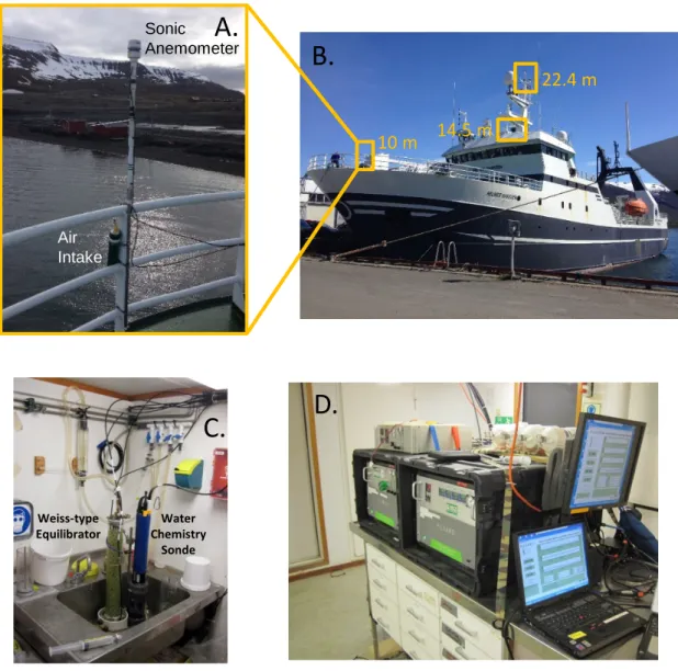
Fig. S1. USGS Gas Analysis System (USGS-GAS). (A) Air intakes and sonic anemometers were placed at (B) 10 m, 14.5 m and 22.4 m above the waterline on the R/V Helmer Hanssen. (C) Seawater from 2 m below the surface was pumped into a Weiss-type equilibrator and EXO2 sonde flow-through chamber. (D) Air
concentrations of methane and CO2from each level were measured for 2 minute intervals with a Picarro G-2301fcavity ring-down spectrometer (CRDS) (on right).
Methane and CO2extracted from the equilibrator were analyzed for concentrations and stable carbon isotopes with a G-2201iCRDS (on left).
Water Chemistry
Sonde Weiss-type
Equilibrator
10 m
A. B.
C. D.
14.5 m
22.4 m
Air Intake
Sonic
Anemometerr
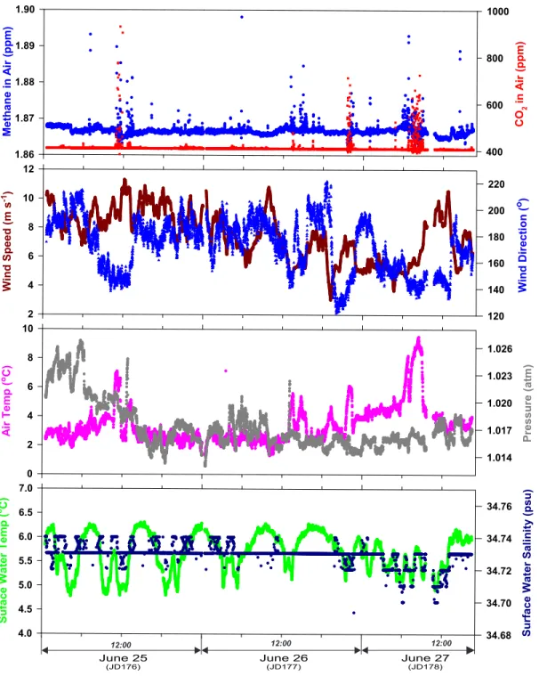
Fig. S2. Atmospheric greenhouse gases, meteorological and surface water time-series data collected during the shallow shelf survey. (a) Methane and CO concentrations at 10 m above the sea 2
surface; (b) Wind speed and direction; (c) Air temperature and pressure; (d) Sea surface temperature (hull- mounted) and salinity. Episodes of high methane and CO generally correspond with higher air 2
temperature and southeasterly (120-140 ) winds originating from Spitsbergen, but were also occasionally o
affected by ship exhaust. To avoid biases related to intake of ship exhaust, median values of 1.865 ppm methane and 407 ppm CO were used for the air concentration component of the gas flux and saturation 2 anomaly calculations. 96.1% of the measured CO values are within 10 ppm of the median and 98.3% of 2 the measured methane values are within 0.05 ppm of the median. Sea-air concentration differences within the seep were about 60 ppm for CO and 6 ppm for methane. Therefore, the effect of using the median 2
values instead of the continuous values for the flux calculations is minimal. Lower sea-surface temperature also corresponds with slightly lower salinity, suggesting the cold, upwelled water is also slightly fresher.
However, the salinity change is at the detection limit of the conductivity sensor such that the measured
A.
C.
B.
12:00 12:00 12:00
June 27
(JD178)
June 26
(JD177)
June 25
(JD176)
−3200
−3200
−3200
−3000
−3000
−2800
−2800
−2600
−2600
−2600
−2400
−2400
−2400
−2400
−2200
−2200
−2200
−2200
−2200
−2200
−2200
−2000
−2000
−2000
−2000
−2000
−2000
−2000
−1800
−1800
−1800
−1800
−1800
−1600
−1600
4˚40' E 5˚00' E 5˚20' E 5˚40' E 6˚00' E 6˚20' E 6˚40' E 7˚00' E 7˚20' E 78˚10' N
78˚15' N 78˚20' N 78˚25' N 78˚30' N 78˚35' N 78˚40' N 78˚45' N
0 1 2 3 4 5
0 km 10 20 km
−3200
−3200
−3200
−3000
−3000
−2800
−2800
−2600
−2600
−2600
−2400
−2400
−2400
−2400
−2200
−2200
−2200
−2200
−2200
−2200
−2200
−2000
−2000
−2000
−2000
−2000
−2000
−2000
−1800
−1800
−1800
−1800
−1800
−1600
−1600
4˚40' E 5˚00' E 5˚20' E 5˚40' E 6˚00' E 6˚20' E 6˚40' E 7˚00' E 7˚20' E 78˚10' N
78˚15' N 78˚20' N 78˚25' N 78˚30' N 78˚35' N 78˚40' N 78˚45' N
−80000 −60000 −40000 −20000 0
0 km 10 20 km
−600
−400
−400
−400
−200
−200
−200
9˚00' E 9˚20' E 9˚40' E 10˚00' E
78˚35' N 78˚40' N
−10000 −7500−5000−2500 0 2500 5000
0 km 2 4 6 km
−600
−400
−400
−400
−200
−200
−200
9˚00' E 9˚20' E 9˚40' E 10˚00' E
78˚35' N 78˚40' N
0 1 2 3 4 5
0 km 2 4 6 km
-2 -1
CH flux (µmol m d )4 WGS84 Mercator Projection
Legend Flare locations
“Area 3 flares”
(Sahling et al., 2014)
“Area 2 flares”
(Sahling et al., 2014)
-2 -1
CO flux (µmol m d )2 WGS84 Mercator Projection
Climate-sensitive gas hydrate area Deep-water gas hydrate area
-2 -1
CH flux (µmol m d )4 WGS84 Mercator Projection
-2 -1
CO flux (µmol m d )2 WGS84 Mercator Projection
A. B.
C. D.
Fig. S3. Sea-air methane (CH ) and CO fluxes from the climate sensitive gas hydrate area (a,c) 4 2
and the deep water gas hydrate system (b,d). Seep locations are indicated with small black dots.
The areas bounded by the yellow and pink lines represent high-intensity climate-sensitive seepage (14).
Data in Table 1 includes the survey lines within the red boxes.
13
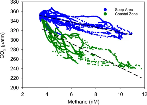
Fig. S4. Surface water pCO (matm) and methane concentration (nM) from the shallow 2 shelf seep area and coastal zone. Methane concentrations negatively correlate with
2 2
pCO in both the seep area (r = 0.61, p < 0.001) and the coastal zone (r = 0.71, p < 2 0.001). Similar patterns of decreasing CO with increasing methane at both of these 2
shallow-shelf settings suggest a similar process. However, greater CO undersaturation in 2
the coastal zone for a range of methane concentrations similar to the seep area suggests methane content does not control the CO dynamics.2
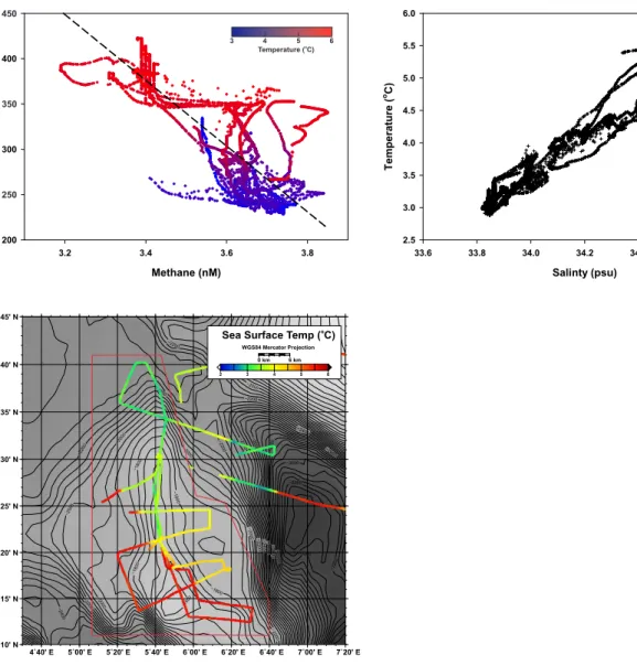
Fig. S5. CO -methane relationship at the deep water gas hydrate site. (A) Methane concentration 2 and pCO negatively correlate (r = 0.61, p< 0.001) at the deep water gas hydrate site (17). Relative to 2 2
the shallow shelf sites, methane concentrations are low, but pCO is similar. Despite the limited 2
quantity of methane in the surface water, higher methane concentrations and lower pCO associate with 2
colder surface waters, as observed on the shelf. (B) The surface waters are most likely a mixture of warmer, higher-salinity water from the West Spitsbergen Current and colder, low-salinity Arctic water (18). (C) Colder surface water is prevalent above the central ridge of the deep-water contourite. A plausible explanation for the greenhouse gas dynamics and oceanographic conditions observed at this site is that upwelling of deep, cold, methane and nutrient-rich water stimulated photosynthesis, as suggested for the shelf seep area. An alternate explanation is the source of the methane was degradation of DMSP produced by marine phytoplankton.
−3200
−3200
−3200
−3000
−3000
−2800
−2800
−2600
−2600
−2600
−2400
−2400
−2400
−2400
−2200
−2200
−2200
−2200
−2200
−2200
−2200
−2000
−2000
−2000
−2000
−2000
−2000
−2000
−1800
−1800
−1800
−1800
−1800
−1600
−1600
4˚40' E 5˚00' E 5˚20' E 5˚40' E 6˚00' E 6˚20' E 6˚40' E 7˚00' E 7˚20' E 78˚10' N
78˚15' N 78˚20' N 78˚25' N 78˚30' N 78˚35' N 78˚40' N 78˚45' N
2 3 4 5 6
Sea Surface Temp ( C)o WGS84 Mercator Projection
0 km 6 km
3 4 5 6
Temperature ( C)o
450
350
250
0:
00:
00
4:
00:
00
8:00:00
12 :00
:00
16 :00
:00
20 :00
:00
0:
00:
00 1
2 3 4 5 6 7
1 2 3 4 5 6 7
0:
00:
00
4:
00:
00
8:
00:00
12 :00
:00
16 :00
:00 1
2 3 4 5 6 7
1 2 3 4 5 6 7 0:
00:
00
4:
00:
00
8:00:00
12 :00
:00
16:00:00
20:00:00
0:00:00 2
3 4 5
2 3 4 5
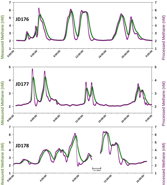
Fig. S6. Raw and processed data comparison. Measured surface methane
concentrations (green) compared to those corrected for the experimentally-determined time constant (τ) (3,4) for the USGS-GAS (purple). JD176-JD178 is the time period for the shallow shelf survey.
JD176
JD177
JD178
Measured Methane (nM) Processed Methane (nM)
Measured Methane (nM) Processed Methane (nM)
Measured Methane (nM) Processed Methane (nM)
no data
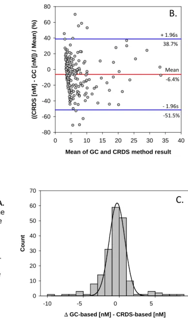
Fig. S7. Bland-Altman agreement analysis. A.
Plot of concentration (nM) differences between the GC-based and CRDS-based methods to describe agreement between measurements. A slight negative bias (-0.48 nM, red line) is observed for the CRDS-based method. Blue lines indicate the difference range for 96% of the 191 comparisons.
B.Differences plotted as a percentage of the measured value. C.Histogram of differences are normally distributed (p < 0.05).
-10 -5 0 5
∆ GC-based [nM] - CRDS-based [nM]
Count
0 10 20 30 40 50 60 70
+ 1.96s
Mean
- 1.96s 38.7%
-51.5%
-6.4%
Mean of GC and CRDS method result
0 5 10 15 20 25 30 35 40
((CRDS [nM] - GC [nM]) / Mean) (%)
-80 -60 -40 -20 0 20 40 60 80
Mean of GC and CRDS method result
0 5 10 15 20 25 30 35 40
CRDS (nM) - GC (nM)
-10 -8 -6 -4 -2 0 2 4 6 8 10
Mean + 1.96s
- 1.96s -0.48
-4.65 3.70
A. B.
C.
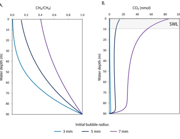
Fig. S8. Results of gas bubble dissolution and stripping simulations for methane seepage at the Svalbard margin (90 m site). Three gas bubble sizes with radii of 3 (light blue), 5 (dark blue), and 7 (purple) mm were simulated. (A) CH4/CH4i denotes the ratio of amount of methane within a gas bubble at a specific depth relative to the amount in a gas bubble at the point of seafloor release. Bubbles with an initial bubble radius of 3 mm (i.e. the average bubble size observed at the WSM (19) lose more than 99%
of their seabed methane content before reaching the sea surface. Hence, methane emissions via direct bubble transport are expected to be small compared to the diffusive outgassing of methane from the surface mixed layer. Only large bubbles with an initial bubble radius of 7 mm are expected to transport significant amounts (~40 %) of seabed methane directly to the sea surface. (B) Amount of CO2 in a gas bubble at a specific depth that has been stripped from seawater during its ascent. Large bubble radii (req
> 7 mm) are required to strip significant amounts of CO2 from seawater and deplete the surface water layer (SWL) in pCO2.
20
Supporting References
1. Wanninkhof R (1992) Relationship between wind speed and gas exchange over the ocean. J Geophys Res‐Oceans 97(C5):7373‐7382.
2. Gulzow W, Rehder G, Schneider B, von Deimling JS, & Sadkowiak B (2011) A new method for continuous measurement of methane and carbon dioxide in surface waters using off‐axis
integrated cavity output spectroscopy (ICOS): An example from the Baltic Sea. Limnol. Oceanogr.
Meth. 9:176‐184.
3. Kodovska FGT, et al. (2016) Dissolved methane and carbon dioxide fluxes in Subarctic and Arctic regions: Assessing measurement techniques and spatial gradients. Earth Planet. Sci. Lett.
436:43‐55.
4. Johnson JE (1999) Evaluation of a seawater equilibrator for shipboard analysis of dissolved oceanic trace gases. Analytica Chimica Acta 395(1‐2):119‐132.
5. Wanninkhof R, Asher WE, Ho DT, Sweeney C, & McGillis WR (2009) Advances in quantifying air‐
sea gas exchange and environmental Forcing. Ann Rev of Mar Sci 1:213‐244.
6. Weiss RF (1974) Carbon dioxide in water and seawater: The solubility of a non‐ideal gas. Marine Chemistry 2:13.
7. Wiesenburg DA & Guinasso NL (1979) Equilibrium solubilities of methane, carbon dioxide, and hydrogen in water and sea‐water. J. Chem. Eng. Data 24(4):356‐360.
8. Ruppel C, Pohlman JW, & Casso M (2017) Data and calculations to support the study of the sea‐
air flux of methane and carbon dioxide on the West Spitsbergen margin in June 2014: U.S.
Geological Survey data release. doi: 10.5066/F7M906V0.
9. Magen C, et al. (2014) A simple headspace equilibration method for measuring dissolved methane. Limnol. Oceanogr. Meth. 12:637‐650.
10. Bland JM & Altman DG (1986) Statistical methods for assessing agreement between two methods of clinical measurement. Lancet 1(8476):307‐310.
11. Fisher RE, et al. (2011) Arctic methane sources: Isotopic evidence for atmospheric inputs.
Geophysical Research Letters 38:6.
12. Vielstadte L, et al. (2015) Quantification of methane emissions at abandoned gas wells in the Central North Sea. Mar. Pet. Geol. 68:848‐860.
13. Boudreau BP (1997) Diagenetic Models and their Implementation: Modeling Transport and Reactions in Aquatic Sediments (Spinger, Berlin) p 414.
14. Duan ZH & Mao SD (2006) A thermodynamic model for calculating methane solubility, density and gas phase composition of methane‐bearing aqueous fluids from 273 to 523 K and from 1 to 2000 bar. Geochim. Cosmochim. Acta 70(13):3369‐3386.
15. Duan ZH, Moller N, & Weare JH (1992) An equation of state for the CH4‐CO2‐H2O system. 1. Pure systems from 0oC to 1000oC and 0 to 8000 bar. Geochim. Cosmochim. Acta 56(7):2605‐2617.
16. Sahling H, et al. (2014) Gas emissions at the continental margin west of Svalbard: mapping, sampling, and quantification. Biogeosciences 11(21):6029‐6046.
17. Johnson JE, et al. (2015) Abiotic methane from ultraslow‐spreading ridges can charge Arctic gas hydrates. Geology 43(5):371‐374.
18. Saloranta TM & Svendsen H (2001) Across the Arctic front west of Spitsbergen: high‐resolution CTD sections from 1998‐2000. Polar Research 20(2):177‐184.
19. Veloso M, Greinert J, Mienert J, & De Batist M (2015) A new methodology for quantifying bubble flow rates in deep water using splitbeam echosounders: Examples from the Arctic offshore NW‐
Svalbard. Limnol. Oceanogr. Meth. 13(6):267‐287.