Predictive analytics and data mining
Charles Elkan elkan@cs.ucsd.edu
May 28, 2013
1
Contents 2
1 Introduction 7
1.1 Limitations of predictive analytics . . . 8
1.2 Opportunities for predictive analytics . . . 10
1.3 Overview . . . 12
2 Predictive analytics in general 15 2.1 Supervised learning . . . 15
2.2 Data validation and cleaning . . . 16
2.3 Data recoding . . . 17
2.4 Missing data . . . 19
2.5 The issue of overfitting . . . 20
3 Linear regression 23 3.1 Interpreting the coefficients of a linear model . . . 25
4 Introduction to Rapidminer 33 4.1 Standardization of features . . . 33
4.2 Example of a Rapidminer process . . . 34
4.3 Other notes on Rapidminer . . . 37
5 Support vector machines 39 5.1 Loss functions . . . 39
5.2 Regularization . . . 41
5.3 Linear soft-margin SVMs . . . 42
5.4 Dual formulation . . . 43
5.5 Nonlinear kernels . . . 44
5.6 Radial basis function kernels . . . 45
5.7 Selecting the best SVM settings . . . 46 2
CONTENTS 3
6 Doing valid experiments 49
6.1 Cross-validation . . . 49
6.2 Cross-validation for model selection . . . 51
7 Classification with a rare class 55 7.1 Thresholds and lift . . . 57
7.2 Ranking examples . . . 58
7.3 Training to overcome imbalance . . . 60
7.4 A case study in classification with a rare class . . . 61
8 Learning to predict conditional probabilities 67 8.1 Isotonic regression . . . 67
8.2 Univariate logistic regression . . . 68
8.3 Multivariate logistic regression . . . 69
8.4 Logistic regression and regularization . . . 70
9 Making optimal decisions 75 9.1 Predictions, decisions, and costs . . . 75
9.2 Cost matrix properties . . . 76
9.3 The logic of costs . . . 77
9.4 Making optimal decisions . . . 78
9.5 Limitations of cost-based analysis . . . 80
9.6 Evaluating the success of decision-making . . . 80
9.7 Rules of thumb for evaluating data mining campaigns . . . 82
10 Learning in nonstandard labeling scenarios 89 10.1 The standard scenario for learning a classifier . . . 89
10.2 Sample selection bias in general . . . 90
10.3 Importance weighting . . . 91
10.4 Covariate shift . . . 92
10.5 Reject inference . . . 93
10.6 Outcomes of treatment . . . 94
10.7 Positive and unlabeled examples . . . 94
10.8 Further issues . . . 97
11 Recommender systems 101 11.1 Applications of matrix approximation . . . 102
11.2 Measures of performance . . . 103
11.3 Additive models . . . 103
11.4 Multiplicative models . . . 104
11.5 Combining models by fitting residuals . . . 106
11.6 Regularization . . . 106
11.7 Further issues . . . 107
12 Text mining 113 12.1 The bag-of-words representation . . . 115
12.2 The multinomial distribution . . . 116
12.3 Training Bayesian classifiers . . . 117
12.4 Burstiness . . . 118
12.5 Discriminative classification . . . 119
12.6 Clustering documents . . . 120
12.7 Topic models . . . 120
12.8 Open questions . . . 121
13 Matrix factorization and applications 127 13.1 Singular value decomposition . . . 128
13.2 Principal component analysis . . . 130
13.3 Latent semantic analysis . . . 131
13.4 Matrix factorization with missing data . . . 133
13.5 Spectral clustering . . . 133
13.6 Graph-based regularization . . . 133
14 Social network analytics 137 14.1 Issues in network mining . . . 138
14.2 Unsupervised network mining . . . 139
14.3 Collective classification . . . 140
14.4 The social dimensions approach . . . 142
14.5 Supervised link prediction . . . 143
15 Interactive experimentation 149 16 Reinforcement learning 151 16.1 Markov decision processes . . . 152
16.2 RL versus cost-sensitive learning . . . 153
16.3 Algorithms to find an optimal policy . . . 154
16.4 Q functions . . . 156
16.5 The Q-learning algorithm . . . 156
16.6 Fitted Q iteration . . . 157
16.7 Representing continuous states and actions . . . 158
16.8 Inventory management applications . . . 160
CONTENTS 5
Bibliography 163
Chapter 1
Introduction
There are many definitions of data mining. We shall take it to mean the application of learning algorithms and statistical methods to real-world datasets. There are nu- merous data mining domains in science, engineering, business, and elsewhere where data mining is useful. We shall focus on applications that are related to business, but the methods that are most useful are mostly the same for applications in science or engineering.
The focus will be on methods for making predictions. For example, the available data may be a customer database, along with labels indicating which customers failed to pay their bills. The goal will then be to predict which other customers might fail to pay in the future. In general, analytics is a newer name for data mining. Predictive analytics indicates a focus on making predictions.
The main alternative to predictive analytics can be called descriptive analytics. In a nutshell, the goal of descriptive analytics is to discover patterns in data. Descriptive and predictive analytics together are often called “knowledge discovery in data” or KDD, but literally that name is a better fit for descriptive analytics. Finding patterns is often fascinating and sometimes highly useful, but in general it is harder to obtain direct benefit from descriptive analytics than from predictive analytics. For example, suppose that customers of Whole Foods tend to be liberal and wealthy. This pattern may be noteworthy and interesting, but what should Whole Foodsdowith the find- ing? Often, the same finding suggests two courses of action that are both plausible, but contradictory. In such a case, the finding is really not useful in the absence of additional knowledge. For example, perhaps Whole Foods should direct its market- ing towards additional wealthy and liberal people. Or perhaps that demographic is saturated, and it should aim its marketing at a currently less tapped, different, group of people?
In contrast, predictions can be typically be used directly to make decisions that 7
maximize benefit to the decision-maker. For example, customers who are more likely not to pay in the future can have their credit limit reduced now. It is important to understand the difference between a prediction and a decision. Data mining lets us make predictions, but predictions are useful to an agentonly if they allow the agent to make decisions that have better outcomes.
Some people may feel that the focus in this course on maximizing profit is dis- tasteful or disquieting. After all, maximizing profit for a business may be at the expense of consumers, and may not benefit society at large. There are several re- sponses to this feeling. First, maximizing profit in general is maximizing efficiency.
Society can use the tax system to spread the benefit of increased profit. Second, in- creased efficiency often comes from improved accuracy in targeting, which benefits the people being targeted. Businesses have no motive to send advertising to people who will merely be annoyed and not respond.
On the other hand, there are some applications of data mining where the profit is positive, but small in comparison with the cost of data mining. In these cases, there might be more social benefit in directing the same effort towards a different objective. For example, in a case study covered below, a charity can spend $70,000 sending solicitations to donors who contribute $84,000 in total. The process has a net benefit for the charity, but the total benefit to society may be negative when the cost to recipients is considered.
1.1 Limitations of predictive analytics
It is important to understand the limitations of predictive analytics. First, in general, one cannot make progress without a dataset for training of adequate size and quality.
Second, it is crucial to have a clear definition of the concept that is to be predicted, and to have historical examples of the concept. Consider for example this extract from an article in the LondonFinancial Timesdated May 13, 2009:
Fico, the company behind the credit score, recently launched a service that pre-qualifies borrowers for modification programmes using their in- house scoring data. Lenders pay a small fee for Fico to refer potential candidates for modifications that have already been vetted for inclusion in the programme. Fico can also help lenders find borrowers that will best respond to modifications and learn how to get in touch with them.
It is hard to see how this could be a successful application of data mining, because it is hard to see how a useful labeled training set could exist. The target concept is “borrowers that will best respond to modifications.” From a lender’s perspective (and Fico works for lenders not borrowers) such a borrower is one who would not pay
1.1. LIMITATIONS OF PREDICTIVE ANALYTICS 9 under his current contract, but who would pay if given a modified contract. Especially in 2009, lenders had no long historical experience with offering modifications to borrowers, so FICO did not have relevant data. Moreover, the definition of the target is based on a counterfactual, that is on reading the minds of borrowers. Data mining cannot read minds.
For a successful data mining application, the actions to be taken based on pre- dictions need to be defined clearly and to have reliable profit consequences. The difference between a regular payment and a modified payment is often small, for ex- ample $200 in the case described in the newspaper article. It is not clear that giving people modifications will really change their behavior dramatically.
For a successful data mining application also, actions must not have major unin- tended consequences. Here, modifications may change behavior in undesired ways.
A person requesting a modification is already thinking of not paying. Those who get modifications may be motivated to return and request further concessions.
Additionally, for predictive analytics to be successful, the training data must be representative of the test data. Typically, the training data come from the past, while the test data arise in the future. If the phenomenon to be predicted is not stable over time, then predictions are likely not to be useful. Here, changes in the general economy, in the price level of houses, and in social attitudes towards foreclosures, are all likely to change the behavior of borrowers in the future, in systematic but unknown ways.
Last but not least, for a successful application it helps if the consequences of actions are essentially independent for different examples. This may be not the case here. Rational borrowers who hear about others getting modifications will try to make themselves appear to be candidates for a modification. So each modification generates a cost that is not restricted to the loss incurred with respect to the individual getting the modification.
An even more clear example of an application of predictive analytics that is un- likely to succeed is learning a model to predict which persons will commit a major terrorist act. There are so few positive training examples that statistically reliable patterns cannot be learned. Moreover, intelligent terrorists will take steps not to fit in with patterns exhibited by previous terrorists [Jonas and Harper, 2006].
A different reason why data mining can be dangerous is that it can lead to missing qualitative issues. An article in theWall Street Journalon March 22, 2012 says
. . . Lulu has gone back to basics. It doesn’t use focus groups, web- site visits or the industry staple–customer-relationship management soft- ware, which tracks purchases. Instead, Ms. Day [the CEO] spends hours each week in Lulu stores observing how customers shop, listening to their complaints, and then using the feedback to tweak product and
Figure 1.1: Top stories as selected by data mining for the Yahoo front page.
stores. “Big data gives you a false sense of security,” says Ms. Day, who spent 20 years at Starbucks Corp., overseeing retail operations in North America and around the world.”
A related issue is that data mining can lead to an ever-increased focus on op- timizing existing processes, at the expense of understanding the broader situation.
For example, for many years Yahoo has used data mining to maximize clicks on the news stories on its front page. As illustrated by Figure 1.1, this has led to the stories becoming more trashy, optimized for a demographic that seeks celebrity news rather than more demanding content.
1.2 Opportunities for predictive analytics
This section discusses criteria for judging the potential success of a proposed appli- cation of data mining. The questions here are listed in a reasonable order in which they should be asked and answered. In tandem with an explanation of each question, there is a discussion of the answers to the questions for a sample application. The application is to predict the success of calls made using a mobile telephone. For each
1.2. OPPORTUNITIES FOR PREDICTIVE ANALYTICS 11 call, the alternative label values are normal termination, call dropped by the network, call dropped by the calling phone, call dropped by the receiving phone, and possibly more.
Does the domain involve numerous individual cases?Data mining and predictive analytics are not directly relevant to making one-off decisions such as selecting the overall strategy of a company or organization. In the example domain, a case is one telephone call, and obviously there are many of these.
Is there a clear objective to be optimized?If it is unclear what the goal is for each case, then there is no definite problem to be solved. Note that the objective is usually from the point of view of a specific agent. For example, if each case is a commercial transaction, then the buyer and seller may have partially conflicting objectives. Data mining is applied to achieve the goals of the agent doing the data mining. In the example domain, the agent doing the data mining is the telephone company, and the goal is for the termination of each call to be successful. While customers have the same general goal, objectives are not perfectly aligned. In particular, each customer is most interested in the success of his or her own calls, but the company may be motivated to prioritize the calls made by its most profitable customers.
Are there actions that influence the objective that can be taken with respect to each case? This is a crucial question. If the agent cannot change the outcomes of cases, then there is no problem to be solved. In the example domain, some avail- able actions are to change the transmission power level of the telephone and/or the base station. In general, a higher power level increases the chance that the call is successful.
Is there an unknown target value that is relevant to the objective that can be predicted for each case? Predictive analytics involves analyzing individual cases in order to predict some relevant characteristic of them that cannot be observed directly at a time when it would be useful to know the characteristic. In the example domain, the target value is whether or not the call will fail.
Is the target value known for numerous historical cases? Yes, after each call its target value is known and can be stored.
Can features of each case be observed that are correlated with the target value?
Yes. These features include the phone model, the weather, the location of the phone and of the base station, the relevant power levels, and derived features such as the distance between the phone and the base station.
Are the cases reasonably independent? That is, does the label of one case not influence strongly the labels of other cases? Yes. The failure of one call does not cause the success or failure of another call.
1.3 Overview
In this course we shall only look at methods that have state-of-the-art accuracy, that are sufficiently simple and fast to be easy to use, and that have well-documented successful applications. We will tread a middle ground between focusing on theory at the expense of applications, and understanding methods only at a cookbook level.
Often, we shall not look at multiple methods for the same task, when there is one method that is at least as good as all the others from most points of view. In particular, for classifier learning, we will look at support vector machines (SVMs) in detail. We will not examine alternative classifier learning methods such as decision trees, neural networks, boosting, and bagging. All these methods are excellent, but it is hard to identify clearly important scenarios in which they are definitely superior to SVMs.
We may also look at random forests, a nonlinear method that is often superior to linear SVMs, and which is widely used in commercial applications nowadays.
Sample CSE 255 Quiz
Instructions. Do this quiz in partnership with exactly one other student. Write both your names at the top of this page. Discuss the answer to the question with each other, and then write your joint answer below the question. Use the back of the page if necessary. It is fine if you overhear what other students say, because you still need to decide if they are right or wrong. You have seven minutes.
Question.Suppose that you work for Apple. The company has developed an un- precedented new product called the iKid, which is aimed at children. Your colleague says “Let’s use data mining on our database of existing customers to learn a model that predicts who is likely to buy an iKid.”
Is your colleague’s idea good or bad? Explain at least one significant specific reason that supports your answer.
Chapter 2
Predictive analytics in general
This chapter explains supervised learning, linear regression, and data cleaning and recoding.
2.1 Supervised learning
The goal of a supervised learning algorithm is to obtain a classifier by learning from training examples. A classifier is something that can be used to make predictions on test examples. This type of learning is called “supervised” because of the metaphor that a teacher (i.e. a supervisor) has provided the true label of each training example.
Each training and test example is represented in the same way, as a row vector of fixed length p. Each element in the vector representing an example is called a feature value. It may be real number or a value of any other type. A training set is a set of vectors with known label values. It is essentially the same thing as a table in a relational database, and an example is one row in such a table. Row, tuple, and vector are essentially synonyms. A column in such a table is often called a feature, or an attribute, in data mining. Sometimes it is important to distinguish between a feature, which is an entire column, and a feature value.
The label y for a test example is unknown. The output of the classifier is a conjecture abouty, i.e. a predictedyvalue. Often each label valueyis a real number.
In this case, supervised learning is called “regression” and the classifier is called a
“regression model.” The word “classifier” is usually reserved for the case where label values are discrete. In the simplest but most common case, there are just two label values. These may be called -1 and +1, or 0 and 1, or no and yes, or negative and positive.
Withntraining examples, and with each example consisting of values forpdif- ferent features, the training data are a matrix withnrows andpcolumns, along with
15
a column vector ofyvalues. The cardinality of the training set isn, while its dimen- sionality isp. We use the notationxij for the value of feature numberjof example numberi. The label of exampleiisyi. True labels are known for training examples, but not for test examples.
2.2 Data validation and cleaning
At the start of a data mining project, typically the analyst does not understand the data fully. Important documentation may be missing, and the data may come from multiple sources that each produced data in a slightly different way. Therefore, the first stage in a data mining project is typically to attempt to detect errors, and to reduce their prevalence. This is often one of the most time-consuming stages of a project, and one of the hardest stages to make routine, since it requires experience, intuition, judgment, and interaction with numerous other people.
Validating data means confirming that it is reliable, while cleaning data means fixing errors in it. Often, it is impossible to be sure whether or not a given data value is correct or not, and if it is incorrect, it is impossible to find the correct value.
Moreover, there may be so many errors that the cost of fixing all of them would be prohibitive. However, it is often possible to gain reasonable confidence that certain data is likely to be correct or incorrect, because it does or does not pass a series of checks. When data is likely to be incorrect, the simplest approach to cleaning it is simply to discard it. While this may introduce biases, more sophisticated cleaning methods are often not beneficial. Generally, more effort should be devoted to data validation than to data repair.
Something that is not exactly data repair is making a feature more meaningful.
For example, suppose that the longevity of a customer is reset to zero when the person changes address. In this case, it may be useful to compute a new feature that measures true longevity regardless of address changes.
Another important type of data cleaning is merging records that refer to the same entity, and should not be separate. The separate records often exist because of variations in representation, such as different ways of writing the same address.
This cleaning process has many names, including record linkage, reduplication, and merge/purge. There are sophisticated methods for it that are outside the scope of this chapter.
A first step in validating data is to examine reports that show basic statistics (minimum, maximum, most frequent values, etc.) for each feature. The reason why each frequent value is frequent should be understood. For example, the social se- curity number 999-99-9999 may be frequent because it means “newly immigrated foreigner.” Features that are supposed to have unique values, i.e. database keys such
2.3. DATA RECODING 17 as id numbers, should be verified to be unique. When the actual value of a feature is supposed to have no intrinsic meaning, this should also be verified. For example, a plot of id numbers may show that certain numerical intervals contain many more numbers than other intervals. If so, the reason for this pattern should be investigated.
A so-called orphan record is one that should have a counterpart elsewhere in the data, but does not. For example, if a transaction record has a certain credit card number, there should be a record elsewhere containing information about the holder of the card, etc. If no such record exists, then the transaction record is an orphan.
Obviously, one should search for orphans and deal with them if they exist.
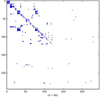
It is often useful to visualize a table of data as a bitmap. In each column, place a 1 for a value of special interest and a 0 for all other values. Then, the analyst can inspect a large table visually. For example, a 1 can be displayed when the actual value is zero, or when the actual value is missing. It is common that a bitmap display shows that there are obvious patterns in data that should not be present.
It can happen that a record is anomalous even though none of its individual fea- ture values is unusual. One way to find anomalous records is to apply a clustering algorithm. The anomalous records may show up as clusters that are small, or even singletons.
Given data containingmfeatures, there arem(m−1)/2possible pairs of fea- tures. Therefore, it can be infeasible to look for anomalies in the correlation between every pair of features. However, it can be worthwhile to look for correlations with specific features where correlations should not exist, or should be small. Id number is an example of a feature that should be uncorrelated with others. Time is a feature where it is important to look for nonlinear patterns. For example, suppose that or- ders for a product peak at the beginning of each month. If so, this may be a genuine pattern, or it may be an artifact due to orders simply being processed in batches.
Another important data validation step is to check that distributions that should be similar really are. For example, a medical dataset may consist of a control group and a treatment group, where each patient was supposedly assigned randomly to one of the two groups. In this case, it is important to check that the distributions of age, previous diagnoses, etc., are all similar for both groups. Often, groups that should be statistically identical turn out to have systematic differences.
2.3 Data recoding
In real-world data, there is a lot of variability and complexity in features. Some fea- tures are real-valued. Other features are numerical but not real-valued, for example integers or monetary amounts. Many features are categorical, e.g. for a student the feature “year” may have values freshman, sophomore, junior, and senior. Usually the
names used for the different values of a categorical feature make no difference to data mining algorithms, but are critical for human understanding. Sometimes categorical features have names that look numerical, e.g. zip codes, and/or have an unwieldy number of different values. Dealing with these is difficult.
It is also difficult to deal with features that are really only meaningful in con- junction with other features, such as “day” in the combination “day month year.”
Moreover, important features (meaning features with predictive power) may be im- plicit in other features. For example, the day of the week may be predictive, but only the day/month/year date is given in the original data. An important job for a human is to think which features may be predictive, based on understanding the application domain, and then to write software that makes these features explicit. No learning algorithm can be expected to discover day-of-week automatically as a function of day/month/year.
Even with all the complexity of features, many aspects are typically ignored in data mining. Usually, units such as dollars and dimensions such as kilograms are omitted. Difficulty in determining feature values is also ignored: for example, how does one define the year of a student who has transferred from a different college, or who is part-time?
Some training algorithms can only handle categorical features. For these, features that are numerical can be discretized. The range of the numerical values is partitioned into a fixed number of intervals that are called bins. The word “partitioned” means that the bins are exhaustive and mutually exclusive, i.e. non-overlapping. One can set boundaries for the bins so that each bin has equal width, i.e. the boundaries are regularly spaced, or one can set boundaries so that each bin contains approximately the same number of training examples, i.e. the bins are “equal count.” Each bin is given an arbitrary name. Each numerical value is then replaced by the name of the bin in which the value lies. It often works well to use ten bins.
Other training algorithms can only handle real-valued features. For these, cat- egorical features must be made numerical. The values of a binary feature can be recoded as 0.0 or 1.0. It is conventional to code “false” or “no” as 0.0, and “true” or
“yes” as 1.0. Usually, the best way to recode a feature that haskdifferent categorical values is to use kreal-valued features. For thejth categorical value, set thejth of these features equal to 1.0 and set allk−1others equal to 0.0.1
Categorical features with many values (say, over 20) are often difficult to deal with. Typically, human intervention is needed to recode them intelligently. For ex- ample, zipcodes may be recoded as just their first one or two letters, since these
1The ordering of the values, i.e. which value is associated withj= 1, etc., is arbitrary. Mathemat- ically, it is sometimes preferable to use onlyk−1real-valued features. For the last categorical value, set allk−1features equal to 0.0. For thejth categorical value wherej < k, set thejth feature value to 1.0 and set allk−1others equal to 0.0.
2.4. MISSING DATA 19 indicate meaningful regions of the United States. If one has a large dataset with many examples from each of the 50 states, then it may be reasonable to leave this as a categorical feature with 50 values. Otherwise, it may be useful to group small states together in sensible ways, for example to create a New England group for MA, CT, VT, ME, NH.
An intelligent way to recode discrete predictors is to replace each discrete value by the mean of the target conditioned on that discrete value. For example, if the average yvalue is 20 for men versus 16 for women, these values could replace the male and female values of a variable for gender. This idea is especially useful as a way to convert a discrete feature with many values, for example the 50 U.S. states, into a useful single numerical feature.
However, as just explained, the standard way to recode a discrete feature with m values is to introduce m−1binary features. With this standard approach, the training algorithm can learn a coefficient for each new feature that corresponds to an optimal numerical value for the corresponding discrete value. Conditional means are likely to be meaningful and useful, but they will not yield better predictions than the coefficients learned in the standard approach. A major advantage of the conditional- means approach is that it avoids an explosion in the dimensionality of training and test examples.
Topics to be explained also: Mixed types, sparse data.
Normalization. After conditional-mean new values have been created, they can be scaled to have zero mean and unit variance in the same way as other features.
When preprocessing and recoding data, it is vital not to peek at test data. If preprocessing is based on test data in any way, then the test data is available indirectly for training, which can lead to overfitting. (See Section 2.5 for an explanation of overfitting.) If a feature is normalized by z-scoring, its mean and standard deviation must be computed using only the training data. Then, later, the same mean and standard deviation values must be used for normalizing this feature in test data.
Even more important, target values from test data must not be used in any way before or during training. When a discrete value is replaced by the mean of the target conditioned on it, the mean must be only oftrainingtarget values. Later, in test data, the same discrete value must be replaced by the same mean of training target values.
2.4 Missing data
A very common difficulty is that the value of a given feature is missing for some training and/or test examples. Often, missing values are indicated by question marks.
However, often missing values are indicated by strings that look like valid known
values, such as 0 (zero). It is important not to treat a value that means missing inadvertently as a valid regular value.
Some training algorithms can handle missingness internally. If not, the simplest approach is just to discard all examples (rows) with missing values. Keeping only examples without any missing values is called “complete case analysis.” An equally simple, but different, approach is to discard all features (columns) with missing val- ues. However, in many applications, both these approaches eliminate too much useful training data.
Also, the fact that a particular feature is missing may itself be a useful predictor.
Therefore, it is often beneficial to create an additional binary feature that is 0 for missing and 1 for present. If a feature with missing values is retained, then it is reasonable to replace each missing value by the mean or mode of the non-missing values. This process is called imputation. More sophisticated imputation procedures exist, but they are not always better.
There can be multiple types of missingness, and multiple codes indicating a miss- ing value. The code NA often means “not applicable” whereas NK means “not known.” Whether or not the value of one feature is missing may depend on the value of another feature. For example, if wind speed is zero, then wind direction is undefined.
2.5 The issue of overfitting
In a real-world application of supervised learning, we have a training set of examples with labels, and a test set of examples with unknown labels. The whole point is to make predictions for the test examples.
However, in research or experimentation we want to measure the performance achieved by a learning algorithm. To do this we use a test set consisting of examples with known labels. We train the classifier on the training set, apply it to the test set, and then measure performance by comparing the predicted labels with the true labels (which were not available to the training algorithm).
It is absolutely vital to measure the performance of a classifier on an independent test set. Every training algorithm looks for patterns in the training data, i.e. corre- lations between the features and the class. Some of the patterns discovered may be spurious, i.e. they are valid in the training data due to randomness in how the train- ing data was selected from the population, but they are not valid, or not as strong, in the whole population. A classifier that relies on these spurious patterns will have higher accuracy on the training examples than it will on the whole population. Only accuracy measured on an independent test set is a fair estimate of accuracy on the
2.5. THE ISSUE OF OVERFITTING 21 whole population. The phenomenon of relying on patterns that are strong only in the training data is called overfitting. In practice it is an omnipresent danger.
Most training algorithms have some settings that the user can choose between.
For ridge regression the main algorithmic parameter is the degree of regularization λ. Other algorithmic choices are which sets of features to use. It is natural to run a supervised learning algorithm many times, and to measure the accuracy of the function (classifier or regression function) learned with different settings. A set of labeled examples used to measure accuracy with different algorithmic settings, in order to pick the best settings, is called a validation set. If you use a validation set, it is important to have a final test set that is independent of both the training set and the validation set. For fairness, the final test set must be used only once. The only purpose of the final test set is to estimate the true accuracy achievable with the settings previously chosen using the validation set.
Dividing the available data into training, validation, and test sets should be done randomly, in order to guarantee that each set is a random sample from the same distri- bution. However, a very important real-world issue is that future real test examples, for which the true label is genuinely unknown, may benota sample from the same distribution.
Please do this assignment in a team of exactly two people. Choose a partner who has a background different from yours.
Install R and Rattle on a computer of your choice, and obtain access to the book Data Mining with Rattle and R. (Online access is free from on campus or using the campus VPN.) Use the example weather dataset included with Rattle.
Examine the Datatab of Rattle. Are the choices made by Rattle aboutIgnore, Ident etc. sensible? If not, make alternative choices. Examine the results of the Exploretab. Are the values of every feature reasonable? If not, what could you do to make the data cleaner?
Using the Test tab, look at the correlations between the featuresPressure9am, Cloud9am, andHumidity9am. Are the three results reasonable? Suggest a real-world explanation for them; look up some basic meteorology if necessary.
Using theModeltab, use three different methods to train a classifier that predicts RainTomorrow: a decision tree, a linear SVM, and logistic regression. Use the default options of Rattle for each method. Using the Evaluate tab, look at six confusion matrices: for each method, one for the training set and one for the test set. Which methods, if any, are underfitting or overfitting the training set?
Next, go back to the Model tab and look at the actual model learned by each method (either a tree or a linear function). For each model, do you see any character- istics of it that suggest that the model may be underfitting or overfitting?
Last but not least, go back to theTransformtab. Try various transformation of the features. Can you find any transformations that improve accuracy of the best model on test data? Is it believable that any improvement would carry over to future test data?
The deliverable for this assignment is a brief report, like a memo. Describe your findings for each step above. Try hard not to fool yourselves, and explain any limitations on the reliability of your conclusions. Do not speculate about future work, and do not explain at length anything that was not successful. Write in the present tense. Organize your report logically, not chronologically. Make the report typeset and format it similarly to this assignment description.
Chapter 3
Linear regression
This chapter explains linear regression, both because it is intrinsically important, and because the issues that arise with linear regression also arise with many other data mining methods.
Letxbe an instance and let y be its real-valued label. For linear regression,x must be a vector of real numbers of fixed length. Remember that this length p is often called the dimension, or dimensionality, ofx. Writex=hx1, x2, . . . , xpi. The linear regression model is
y=b0+b1x1+b2x2+. . .+bpxp.
The righthand side above is called a linear function of x. The linear function is defined by its coefficients b0 to bp. These coefficients are the output of the data mining algorithm.
The coefficientb0 is called the intercept. It is the value of y predicted by the model ifxi= 0for alli. Of course, it may be completely unrealistic that all features xihave value zero. The coefficientbiis the amount by which the predictedy value increases if xi increases by 1, if the value of all other features is unchanged. For example, suppose xi is a binary feature where xi = 0 means female and xi = 1 means male, and supposebi =−2.5. Then the predictedy value for males is lower by 2.5, everything else being held constant.
Suppose that the training set has cardinalityn, i.e. it consists of nexamples of the form hxi, yii, wherexi = hxi1, . . . , xipi. Letbbe any set of coefficients. The predicted value forxiis
ˆ
yi=f(xi;b) =b0+
p
X
j=1
bjxij.
23
The semicolon in the expressionf(xi;b)emphasizes that the vectorxi is a variable input, whilebis a fixed set of parameter values. If we definexi0 = 1for everyi, then we can write
ˆ yi =
p
X
j=0
bjxij.
The constantxi0 = 1can be called a pseudo-feature.
Finding the optimal values of the coefficients b0 tobp is the job of the training algorithm. To make this task well-defined, we need a definition of what “optimal”
means. The standard approach is to say that optimal means minimizing the sum of squared errors on the training set, where the squared error on training exampleiis (yi−yˆi)2. The training algorithm then finds
ˆb=argminb
n
X
i=1
(f(xi;b)−yi)2. The objective functionP
i(yi−P
jbjxij)2 is called the sum of squared errors, or SSE for short. Note that during training the ndifferentxi andyi values are fixed, while the parametersbare variable.
The optimal coefficient valuesˆbare not defined uniquely if the numbernof train- ing examples is less than the numberpof features. Even ifn > pis true, the optimal coefficients have multiple equivalent values if some features are themselves related linearly. Here, “equivalent” means that the different sets of coefficients achieve the same minimum SSE. For an intuitive example, suppose features 1 and 2 are tem- perature measured in degrees Celsius and degrees Fahrenheit respectively.1 Then x2 = 32 + 9(x1/5) = 32 + 1.8x1, and the same model can be written in many different ways:
• y=b0+b1x1+b2x2
• y=b0+b1x1+b2(32 + 1.8x1) = [b0+ 32b2] + [b1(1 + 1.8b2)]x1+ 0x2 and an infinite number of other ways. In the extreme, suppose x1 = x2. Then all modelsy =b0+b1x1+b2x2are equivalent for whichb1+b2equals a constant.
When two or more features are approximately related linearly, then the true val- ues of the coefficients of those features are not well determined. The coefficients obtained by training will be strongly influenced by randomness in the training data.
Regularization is a way to reduce the influence of this type of randomness. Consider
1Having two features which are in fact duplicates, but measured in different ways, is a common data quality problem. The problem can be hard to detect, because there maybe differing noise in the measurements, and/or some of the duplicate measurements may be missing.
3.1. INTERPRETING THE COEFFICIENTS OF A LINEAR MODEL 25 all modelsy=b0+b1x1+b2x2for whichb1+b2 =c. Among these models, there is a unique one that minimizes the functionb21+b22. This model hasb1 =b2 =c/2. We can obtain it by setting the objective function for training to be the sum of squared errors (SSE) plus a function that penalizes large values of the coefficients. A sim- ple penalty function of this type isPp
j=1b2j. A parameterλcan control the relative importance of the two objectives, namely SSE and penalty:
ˆb=argminb 1 n
n
X
i=1
(yi−yˆi)2 + λ1 p
p
X
j=1
b2j.
If λ = 0 then one gets the standard least-squares linear regression solution. As λincreases, the penalty on large coefficients gets stronger, and the typical values of coefficients get smaller. The parameterλis often called the strength of regularization.
The fractions1/nand1/pdo not make an essential difference. They can be used to make the numerical value ofλeasier to interpret.
The penalty functionPp
j=1b2j is the square of theL2norm of the vectorb. Using it for linear regression is called ridge regression. Any penalty function that treats all coefficients bj equally, like the L2 norm, is sensible only if the typical magnitudes of the values of each feature are similar; this is an important motivation for data normalization. Note that in the formula Pp
j=1b2j the sum excludes the intercept coefficientb0. One reason for doing this is that the targetyvalues are typically not normalized.
3.1 Interpreting the coefficients of a linear model
It is common to desire a data mining model that is interpretable, that is one that can be used not only to make predictions, but also to understand patterns, and even possible mechanisms, in the phenomenon that is being studied. Linear models, whether for re- gression or for classification as described in later chapters, do appear interpretable at first sight. However, much caution is needed when attempting to derive conclusions from numerical coefficients.
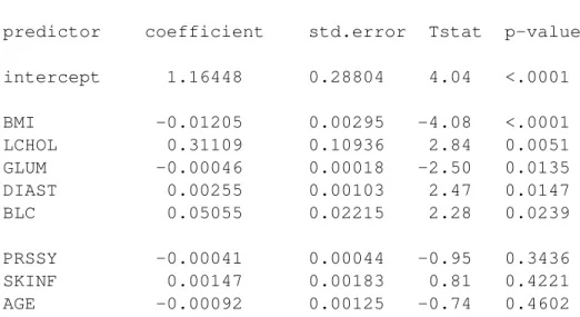
Consider the linear regression model in Table 3.1 for predicting high-density cholesterol (HDL) levels.2 The example illustrates at least two crucial issues. First, if predictors are collinear, then one may appear significant and the other not, when in fact both are significant or both are not. Above, diastolic blood pressure is statisti- cally significant, but systolic is not. This may possibly be true for some physiological reason. But it may also be an artifact of collinearity.
2HDL cholesterol is considered beneficial and is sometimes called “good” cholesterol. Source:
http://www.jerrydallal.com/LHSP/importnt.htm. Predictors have been reordered from most to least statistically significant, as measured byp-value.
predictor coefficient std.error Tstat p-value intercept 1.16448 0.28804 4.04 <.0001 BMI -0.01205 0.00295 -4.08 <.0001
LCHOL 0.31109 0.10936 2.84 0.0051
GLUM -0.00046 0.00018 -2.50 0.0135
DIAST 0.00255 0.00103 2.47 0.0147
BLC 0.05055 0.02215 2.28 0.0239
PRSSY -0.00041 0.00044 -0.95 0.3436
SKINF 0.00147 0.00183 0.81 0.4221
AGE -0.00092 0.00125 -0.74 0.4602
Table 3.1: Linear regression model to predict HDL cholesterol levels. From most to least statistically significant, the predictors are body mass index, the log of to- tal cholesterol, glucose metabolism, diastolic blood pressures, and vitamin C level in blood. Three predictors are not statistically significant: systolic blood pressure, skinfold thickness, and age in years.
Second, a predictor may be practically important, and statistically significant, but still useless for interventions. This happens if the predictor and the outcome have a common cause, or if the outcome causes the predictor. Above, vitamin C is statistically significant. But it may be that vitamin C is simply an indicator of a generally healthy diet high in fruits and vegetables. If this is true, then merely taking a vitamin C supplement will not cause an increase in HDL level.
A third crucial issue is that a correlation may disagree with other knowledge and assumptions. For example, vitamin C is generally considered beneficial or neutral.
If lower vitamin C was associated with higher HDL, one would be cautious about believing this relationship, even if the association was statistically significant.
Exercises
1.
Suppose you are building a model to predict how many dollars someone will spend at Sears. You know the gender of each customer, male or female. Since you are using linear regression, you must recode this discrete feature as continuous. You decide to use two real-valued features, x11 andx12. The coding is a standard “one ofn”
scheme, as follows:
gender x11 x12
male 1 0
female 0 1
Learning from a large training set yields the model y=. . .+ 15x11+ 75x12+. . .
Dr. Roebuck says “Aha! The average woman spends $75, but the average man spends only $15.”
(a) Explain why Dr. Roebuck’s conclusion is not valid. The model only predicts spending of$75 for a woman if all other features have value zero. This may not be true for the average woman. Indeed it will not be true for any woman, if features such as “age” are not normalized.
(b) Explain what conclusion can actually be drawn from the numbers 15 and 75.
The conclusion is that if everything else is held constant, then on average a woman will spend$60 more than a man. Note that if some feature values are systematically different for men and women, then even this conclusion is not useful, because then it is not reasonable to hold all other feature values constant.
(c) Explain a desirable way to simplify the model. The two features x11 and x12 are linearly related. Hence, they make the optimal model be undefined, in the absence of regularization. It would be good to eliminate one of these two features.
The expressiveness of the linear model would be unchanged.
2.
Suppose that you are training a model to predict how many transactions a credit card customer will make. You know the education level of each customer. Since you are using linear regression, you recode this discrete feature as continuous. You decide to use two real-valued features,x37andx38. The coding is a “one of two” scheme, as follows:
x37 x38
college grad 1 0
not college grad 0 1 Learning from a large training set yields the model
y=. . .+ 5.5x37+ 3.2x38+. . .
(a) Dr. Goldman concludes that the average college graduate makes 5.5 transac- tions. Explain why Dr. Goldman’s conclusion is likely to be false. The model only predicts 5.5 transactions if all other features, including the intercept, have value zero.
This may not be true for the average college grad. It will certainly be false if features such as “age” are not normalized.
(b) Dr. Sachs concludes that being a college graduate causes a person to make 2.3 more transactions, on average. Explain why Dr. Sachs’ conclusion is likely to be false also. First, if any other feature have different values on average for men and women, for example income, then5.5−3.2 = 2.3 is not the average difference in predictedyvalue between groups. Said another way, it is unlikely to be reasonable to hold all other feature values constant when comparing groups.
Second, even if 2.3 is the average difference, one cannot say that this difference is caused by being a college graduate. There may be some other unknown common cause, for example.
3.
Suppose that you are training a model (a classifier) to predict whether or not a grad- uate student drops out. You have enough positive and negative training examples, from a selective graduate program. You are training the model correctly, without overfitting or any other mistake. Assume further that verbal ability is a strong causal influence on the target, and that the verbal GRE score is a good measure of verbal ability.
Explain two separate reasonable scenarios where the verbal GRE score, despite all the assumptions above being true, does not have strong predictive power in a trained model.
CSE 255 assignment due on April 16, 2013
As before, do this assignment in a team of exactly two people, and choose a partner with a background different from yours. You may keep the same partner, or change.
Download the filecup98lrn.zipfrom fromhttp://archive.ics.uci.
edu/ml/databases/kddcup98/kddcup98.html. Read the associated doc- umentation. Load the data into R, or other software for data mining. Select the 4843 records that have feature TARGET_B=1. Now, build a linear regression model to predict the fieldTARGET_Das accurately as possible. Use root mean squared error (RMSE) as the definition of error. Do a combination of the following:
• Discard useless features.
• Process missing feature values in a sensible way.
• Recode non-numerical features as numerical.
• Add transformations of existing features.
• Compare different strengths of ridge (L2) regularization.
Do the steps above repeatedly in order to explore alternative ways of using the data.
The outcome should be the best model that you can find that uses 10 or fewer of the original features. After recoding features, you will likely have more than 10 derived features, but these should all be based on at most 10 of the original features. Use cross-validation to evaluate each model that you consider. The RMSE of your final model (on validation folds, not on training folds) should be less than $9.00.
You should discard useless features quickly; for this assignment, you do not need to use a systematic process to identify these. If you normalize all input features, and you use strong L2 regularization (ridge parameter 107 perhaps), then the re- gression coefficients will be an (imperfect) indicator of the relative importance of features. L1 regularization is an alternative way of identifying important features quickly. Construct the best model that you can, including choosing the best strength ofL2regularization for the features that you retain.
After you have found a final model that you expect to generalize well, use ten- fold cross-validation to estimate its accuracy. Write down what RMSE you ex- pect to achieve on future data. Then, run this model on the independent test set cup98val.zip. For the approximately 5% of records for whichTARGET_B= 1, compute the RMSE of your predictions with respect to theTARGET_Dvalues in the filevaltargt.txt. Be sure to write down your expected RMSE in advance, to help avoid fooling yourselves. Note that you must use theCONTROLNfeature to join thecup98val.zipandvaltargt.txtfiles correctly.
validity or reliability of your results. Explain the RMSE that you expected on the test data, and the RMSE that you observed. Include your final regression model.
Comments
To make your work more efficient, be sure to save the 4843 records in a format that your software can reload quickly. You can use three-fold cross-validation during development to save time, but do use ten-fold cross-validation to evaluate the RMSE of your final chosen model.
It is typically useful to rescale predictors to have mean zero and variance one.
However, it loses interpretability to rescale the target variable. Note that if all pre- dictors have mean zero, then the intercept of a linear regression model is the mean of the target, $15.6243 here. The intercept should usually not be regularized.
The assignment specifically asks you to report root mean squared error, RMSE.
Mean squared error, MSE, is an alternative, but whichever is chosen should be used consistently. In general, do not confuse readers by switching between multiple mea- sures without a good reason, and do follow precise instructions precisely.
As is often the case, good performance can be achieved with a very simple model.
The most informative single feature isLASTGIFT, the dollar amount of the person’s most recent gift. A model based on just this single feature achieves RMSE of $9.98.
The assignment asks you to produce a final model based on at most 10 of the original features. It is not a good idea to begin by choosing a subset of the 480 original features based on human intuition, because intuition is unreliable. It is also not a good idea to eliminate automatically features with missing values.
Many tools for data mining have operators that search for highly predictive sub- sets of variables. These operators tend to have two major problems. First, they are too slow to be used on a large initial set of variables, so it is easy for human intuition to pick an initial set that is not good. Second, they try a very large number of alter- native subsets of variables, and pick the one that performs best on some training or tuning set. Because of the high number of alternatives considered, the chosen subset is likely to overfit substantially the training or tuning set.
It is important that you applyonly onemodel to the final test data. After you do this, you may be tempted to go back and train a different model, and to apply that to the cup98val.ziptest data. However, doing so would be cheating, because it would allow the test data to influence the training process, which would lead to overfitting the test data, and hence to an overoptimistic estimate of accuracy. More generally, even for a task as simple and well-defined as the one in this assignment,
3.1. INTERPRETING THE COEFFICIENTS OF A LINEAR MODEL 31 it is easy to fool yourselves, and your readers, about the correctness and success of your work. Do apply critical thinking, and aim for simplicity and clarity.
Chapter 4
Introduction to Rapidminer
By default, many Java implementations allocate so little memory that Rapidminer will quickly terminate with an “out of memory” message. This is not a problem with Windows 7, but otherwise, launch Rapidminer with a command like
java -Xmx1g -jar rapidminer.jar where1gmeans one gigabyte.
4.1 Standardization of features
The recommended procedure is as follows, in order.
• Normalize all numerical features to have mean zero and variance 1.
• Convert each nominal feature withkalternative values intokdifferent binary features.
• Optionally, drop all binary features with fewer than 100 examples for either binary value.
• Convert each binary feature into a numerical feature with values 0.0 and 1.0.
It is not recommended to normalize numerical features obtained from binary features.
The reason is that this normalization would destroy the sparsity of the dataset, and hence make some efficient training algorithms much slower. Note that destroying sparsity is not an issue when the dataset is stored as a dense matrix, which it is by default in Rapidminer.
Normalization is also questionable for variables whose distribution is highly un- even. For example, almost all donation amounts are under $50, but a few are up
33
to $500. No linear normalization, whether by z-scoring or by transformation to the range 0 to 1 or otherwise, will allow a linear classifier to discriminate well between different common values of the variable. For variables with uneven distributions, it is often useful to apply a nonlinear transformation that makes their distribution have more of a uniform or Gaussian shape. A common transformation that often achieves this is to take logarithms. A useful trick when zero is a frequent value of a variable x is to use the mappingx 7→ log(x+ 1). This leaves zeros unchanged and hence preserves sparsity.
Eliminating binary features for which either value has fewer than 100 training examples is a heuristic way to prevent overfitting and at the same time make training faster. It may not be necessary, or beneficial, if regularization is used during training.
If regularization is not used, then at least one binary feature must be dropped from each set created by converting a multivalued feature, in order to prevent the existence of multiple equivalent models. For efficiency and interpretability, it is best to drop the binary feature corresponding to the most common value of the original multivalued feature.
If you have separate training and test sets, it is important to do all preprocessing in a perfectly consistent way on both datasets. The simplest is to concatenate both sets before preprocessing, and then split them after. However, concatenation allows information from the test set to influence the details of preprocessing, which is a form of information leakage from the test set, that is of using the test set during training, which is not legitimate.
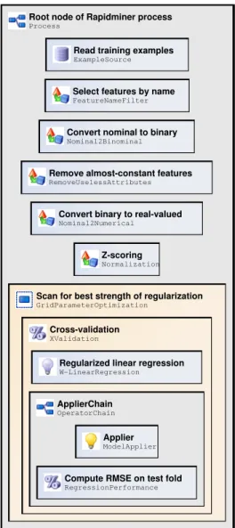
4.2 Example of a Rapidminer process
Figure 4.2 shows a tree structure of Rapidminer operators that together perform a standard data mining task. The tree illustrates how to perform some common sub- tasks.
The first operator is ExampleSource. “Read training example” is a name for this particular instance of this operator. If you have two instances of the same operator, you can identify them with different names. You select an operator by clicking on it in the left pane. Then, in the right pane, the Parameters tab shows the arguments of the operator. At the top there is an icon that is a picture of either a person with a red sweater, or a person with an academic cap. Click on the icon to toggle between these. When the person in red is visible, you are in expert mode, where you can see all the parameters of each operator.
The example source operator has a parameter named attributes. Normally this is file name with extension “aml.” The corresponding file should contain a schema definition for a dataset. The actual data are in a file with the same name with exten-
4.2. EXAMPLE OF A RAPIDMINER PROCESS 35
Root node of Rapidminer process Process
Read training examples ExampleSource
Select features by name FeatureNameFilter
Convert nominal to binary Nominal2Binominal
Remove almost-constant features RemoveUselessAttributes
Convert binary to real-valued Nominal2Numerical
Z-scoring Normalization
Scan for best strength of regularization GridParameterOptimization
Cross-validation XValidation
Regularized linear regression W-LinearRegression
ApplierChain OperatorChain
Applier ModelApplier
Compute RMSE on test fold RegressionPerformance
Figure 4.1: Rapidminer process for regularized linear regression.
sion “dat.” The easiest way to create these files is by clicking on “Start Data Loading Wizard.” The first step with this wizard is to specify the file to read data from, the character that begins comment lines, and the decimal point character. Ticking the box for “use double quotes” can avoid some error messages.
In the next panel, you specify the delimiter that divides fields within each row of data. If you choose the wrong delimiter, the data preview at the bottom will look wrong. In the next panel, tick the box to make the first row be interpreted as field names. If this is not true for your data, the easiest is to make it true outside Rapid- miner, with a text editor or otherwise. When you click Next on this panel, all rows of data are loaded. Error messages may appear in the bottom pane. If there are no errors and the data file is large, then Rapidminer hangs with no visible progress. The same thing happens if you click Previous from the following panel. You can use a CPU monitor to see what Rapidminer is doing.
The next panel asks you to specify the type of each attribute. The wizard guesses this based only on the first row of data, so it often makes mistakes, which you have to fix by trial and error. The following panel asks you to say which features are special.
The most common special choice is “label” which means that an attribute is a target to be predicted.
Finally, you specify a file name that is used with “aml” and “dat” extensions to save the data in Rapidminer format.
To keep just features with certain names, use the operator FeatureNameFilter. Let the argumentskip_features_with_namebe.*and let the argumentexcept_
features_with_nameidentify the features to keep. In our sample process, it is
(.*AMNT.*)|(.*GIFT.*)(YRS.*)|(.*MALE)|(STATE)|(PEPSTRFL)|(.*GIFT)
|(MDM.*)|(RFA_2.*).
In order to convert a discrete feature withk different values intokreal-valued 0/1 features, two operators are needed. The first isNominal2Binominal, while the second is Nominal2Numerical. Note that the documentation of the latter operator in Rapidminer is misleading: it cannot convert a discrete feature into multi- ple numerical features directly. The operatorNominal2Binominalis quite slow.
Applying it to discrete features with more than 50 alternative values is not recom- mended.
The simplest way to find a good value for an algorithm setting is to use the XValidationoperator nested inside theGridParameterOptimizationop- erator. The way to indicate nesting of operators is by dragging and dropping. First create the inner operator subtree. Then insert the outer operator. Then drag the root of the inner subtree, and drop it on top of the outer operator.
4.3. OTHER NOTES ON RAPIDMINER 37
4.3 Other notes on Rapidminer
Reusing existing processes.
Saving datasets.
Operators from Weka versus from elsewhere.
Comments on specific operators: Nominal2Numerical, Nominal2Binominal, Re- moveUselessFeatures.
Eliminating non-alphanumerical characters, using quote marks, trimming lines, trimming commas.
Chapter 5
Support vector machines
This chapter explains support vector machines (SVMs). The SVMs described here are called soft margin SVMs, for reasons that will be explained later. This variant is by far the most commonly used in practice. The chapter discusses linear and nonlinear kernels. It also discusses preventing overfitting via regularization.
We have seen how to use linear regression to predict a real-valued label. Now we will see how to use a similar model to predict a binary label. In later chapters, where we think probabilistically, it will be convenient to assume that a binary label takes on true values 0 or 1. However, in this chapter it will be convenient to assume that the labelyhas true value either+1or−1.
5.1 Loss functions
Letxbe an instance (a numerical vector of dimensiond), letybe its true label, and let f(x) be a prediction. Assume that the prediction is real-valued. If we need to convert it into a binary prediction, we will threshold it at zero:
ˆ
y= 2·I(f(x)≥0)−1
whereI()is an indicator function that is 1 if its argument is true, and 0 if its argument is false.
A so-called loss functionl(·,·) measures how good the prediction is. Typically loss functions do not depend directly onx, and a loss of zero corresponds to a perfect prediction, while otherwise loss is positive. The most obvious loss function is
l(f(x), y) =I(ˆy6=y)
which is called the 0-1 loss function. The usual definition of accuracy uses this loss function. However, it has undesirable properties. First, it loses information: it does
39
not distinguish between predictions f(x) that are almost right, and those that are very wrong. Second, mathematically, its derivative with respect to the value off(x) is either undefined or zero. This makes the 0/1 loss function difficult to use in training algorithms that try to minimize loss by adjusting parameter values using derivatives.
A loss function that is preferable in several ways is squared error:
l(f(x), y) = (f(x)−y)2.
This function is infinitely differentiable everywhere, and does not lose information when the predictionf(x)is real-valued. However, it says that the predictionf(x) = 1.5is as undesirable asf(x) = 0.5when the true label isy = 1. Intuitively, if the true label is+1, then a prediction with the correct sign that is greater than 1 should not be considered incorrect.
The following loss function, which is called hinge loss, satisfies the intuition just suggested:
l(f(x),−1) = max{0,1 +f(x)}
l(f(x),+1) = max{0,1−f(x)}
To understand this loss function, look at a figure showing the lossl(f(x),−1)for a negative example as a function of the outputf(x)of the classifier. The loss is zero, which is the best case, as long as the predictionf(x)≤ −1. The further awayf(x) is from −1in the wrong direction, meaning the more f(x) is bigger than −1, the bigger the loss. There is a similar but opposite pattern when the true label isy= +1.
It is mathematically convenient, but less intuitive, to write the hinge loss function as l(f(x), y) = max{0,1−yf(x)}.
Using hinge loss is the first major insight behind SVMs. An SVM classifier f is trained to minimize hinge loss. The training process aims to achieve predictions f(x)≥1for all training instancesxwith true labely = +1, and to achieve predic- tionsf(x) ≤ −1 for all training instancesxwith y = −1. Note that we have not yet said anything about what the space of candidate functionsf is. Overall, training seeks to classify points correctly, but it does not seek to make predictions be exactly +1or−1. In this sense, the training process intuitively aims to find the best pos- sible classifier, without trying to satisfy any unnecessary additional objectives also.
The training process does attempt to distinguish clearly between the two classes, by predictions that are inside the interval(−1,+1).