Active Matter Physics
Submission due: 3:00 p.m. on May 04, 2021
Exercise Sheet 2
2.1
• Checking whether a system fulfills detailed balance, i.e., verifying whether the relation π(σ0 →σ)P(σ0) =π(σ→σ0)P(σ) (1) holds true for all σ, σ0, is not always a trivial task, since the stationary probabilities P(σ) and P(σ0) might not be known exactly. The Kolmogorov criterion could appear useful in these situations. It states that a system fulfills the detailed balance condition in Equation (1) if and only if for all cyclesσ1→σ2→...→σk the respective transition rates satisfy
π(σ1→σ2)π(σ2→σ3)...π(σk →σ1) =π(σ1→σk)π(σk →σk−1)...π(σ2→σ1). (2) Proof this criterion. (Hint: For the “backward direction” of the proof, i.e., for the case in which the Kolmogorov criterion holds true, define the (unnormalized) stationary probability
P(σ2) :=P(σ1)π(σ1→σ2)
π(σ2→σ1) (3)
for a stateσ2which is connected to a given stateσ1with (unnormalized) probabilityP(σ1).)
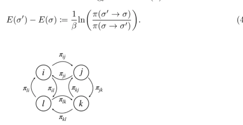
• According to the Kolmogorov criterion, which relation has to be fulfilled for the stationary Markov chain in Figure 1 by traversing the loop i to j to l to k to i? (Abbreviation:
πxy :=π(x→y) withx, y∈ {i, j, k, l}.)
• Show that for a stateσin the stationary state its corresponding stationary probabilityP(σ) has the form of a Boltzmann factor. A suitable energy functionE(σ) can be defined via
E(σ0)−E(σ) := 1 βln
π(σ0→σ) π(σ→σ0)
. (4)
i j
k l
πij πji
πjk πkj πkl πlk πli πil
Figure 1: Discrete-time Markov chain with four states.
2.2
• Consider a stochastic process (X(t))t≥0 which obeys the stochastic differential equation dX(t) =−X(t)dt
1 +t +dW(t)
1 +t , X0= 0, (5)
whereW(t)t≥0 is a (standard) Wiener process (also known as Brownian motion). Solve this stochastic differential equation following the attaching recipe:
1
1. Apply It¯o’s lemma to a functionF :R+×R→R, (t, X(t))→F(t, X(t)):
dF =
∂F
∂Xa(t) +∂F
∂t +1 2
∂2F
∂X2b(t)2
dt+∂F
∂Xb(t)dW(t), (6) where (a(t))t≥0and (b(t))t≥0are stochastic processes occurring in the general stochastic differential equation dX(t) =a(t)dt+b(t)dW(t).
2. ChooseF(t, X(t)) such that the coefficients of dtand dW(t) in Equation 6 are functions oftalone.
3. Choose the parameters of your option for F(t, X(t)) from the previous step such that dF(t, X(t)) = dW(t) holds true in Equation 6.
4. Solve Equation 5.
• The positionx(t) of a particle executing a uniform random walk is the solution of the stochas- tic differential equation
dx(t) =µdt+σdW(t), x(0) =x0, (7)
where µ andσ are constants. Find the probability density f(t, x(t)) of x(t) at timet > 0.
You may use the following hints:
1. Set up the corresponding Fokker–Planck equation forf(t, x(t)). What is the respective initial condition?
2. Apply the method of Fourier transformation as well as its properties to solve this partial differential equation.
2.3
The two files “data_passive_particle” and “data_active_particle” contain measured position data of a passive random walker as well as an active random walker as described in the lecture, respec- tively, which were recorded at a time lag of 50 ms between two successive measurement points and atT = 300 K. These position data are given inµm (the angular data of the active particle are of no further interest for this task). Both particles have a radius of 500 nm. Furthermore, the active particle is propelled at a velocity ofv= 8µm/s. Using these data, numerically compute/visualize
• the position distribution of both particles in one plot (i.e., plot anx-y-graph),
• the one-dimensional step size distributions in thex- andy-directions for both types of par- ticles (Hint: step size, for example, inx-direction: ∆x(t) =x(t+ 1)−x(t)),
• the two-dimensional step size distributions for both types of particles as well as
• their mean squared displacements (in one plot) and compare them to their theoretical pre- dictions (η = 10−3Pa·s).
2