Chapter 5
Approaches to Quantum Chaos
In this chapter, we shall present semiclassical methods that were devel- opped since about 1970 in order to describe the quantum-mechanical energy spectrum of a classically chaotic system. We essentially follow Gutzwiller (1990) and Berry & Mount (1972).
The central tool is the so-called trace formula, first derived by GUTZWILLER in 1967. Thie formula relates the quantum-mechanical en- ergy level densityn(E)to the spatial trace of the Green operator:
n(E) = 1
⇡
Z
dqImG(q, q;E) (5.1) We get a tractable (though still complicated) expression when the semiclas- sical approximation for the Green function is used in this formula. In the following, we first prove (5.1) using elementary quantum mechanics and then approximate the Green function.
5.1 Green operator and function
For a quantum-mechanical system with HAMILTON operatorH, the Gˆ REEN operator is defined by
⇣E Hˆ⌘Gˆ =1
This equation is formally solved. Taking a complex energy E+ i 0 with a positive (infinitesimal) imaginary part, we find
Im ˆG= ⇡1 ⇣E Hˆ⌘
In the position representation, we have the expansion G(qB, qA) = hqB|Gˆ|qAi=X
n
n(qB) n⇤(qA) E En
where theEn are the energy eigenvalues and n(q)the corresponding nor- malised wave functions. Putting hereqB = qA = q and integrating over q,
we find Z
dq G(q, q) = X
n
1 E En
For an energyE+ i 0, the imaginary part gives 1
⇡Im
Z
dq G(q, q) =X
n
(E En) = n(E) (5.2) This is the energy level density: a series of peaks at the energy eigenval- ues. For a continuous spectrum, the sum overn is actually an integral, and the level density becomes a continuous function.
5.2 The semiclassical propagator
We start with the semiclassical approximation to the time-dependent prop- agator.
The quantum-mechanical propagator K(B, A) =K(qB, t;qA,0)is equal to the probability amplitude that a particle reaches the position qB at time tafter starting from a position eigenstate localised inqAat time0.
The propagator thus solves the SCHRODINGER¨ equation i¯h@t+ ¯h2
2m B V(qB)
!
K = 0 with the initial condition
limt!0K(B, A) = (qB qA) (5.3) VAN VLECK propagator
As early as 1928, VAN VLECKwrote the followingAnsatzfor the propagator.
It is inspired from the hydrodynamical formulation of the SCHRODINGER¨
equation
K(B, A) = 1 (2⇡i¯h)D/2
X
r
q
Crexp i [R(B, A)/¯h µr⇡/2] (5.4) To leading order in ¯h ! 0, we get from the SCHRODINGER¨ equation the HAMILTON–JACOBIequation
@tR+ 1
2m(rBR)2 +V(qB) = 0
Its solution is the action R (also called ‘HAMILTON’s principal function’).
This can be calculated from classical dynamics.
In next-to-leading order, we find the continuity equation
@tCr+ 1
mrB·(CrrBR) = 0
where Cr plays the role of a (probability) density, and the momentum is pB = rBR(B, A)(standard relation from LAGRANGE mechanics). The am- plitudeCr can hence also be calculated from classical dynamics.
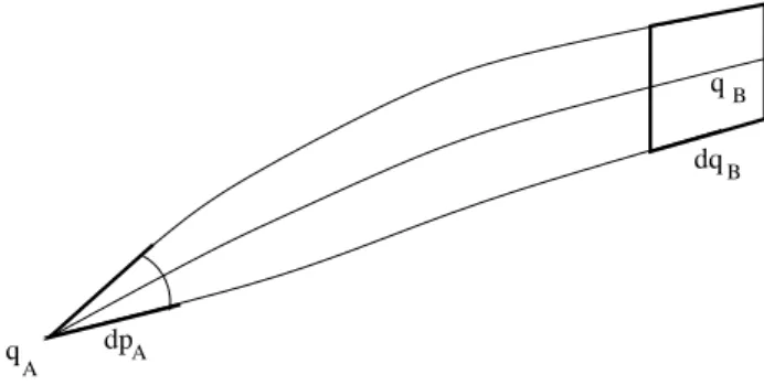
It is easy to derive an explicit formula for the density in terms of the classical trajectories. Recall that the quantity
|K(B, A)|2dqB
gives the probability to reach a volume element dqB around the final po- sition qB. Since probability is conserved along the classical trajectories, this probability is equal to the probability to start with the correct initial momentumpA(see figure 5.1). This is given by
dp
dqB qB
qA A
Figure 5.1: Final positionqB and initial momentumpA.
g(pA)dpA= dpA
(2⇡¯h)D
with the momentum distribution g(pA). For an initially localised particle, we know from quantum mechanics that its momentum distribution is flat.
We thus find
|K(B, A)|2 = 1 (2⇡¯h)D
@(pA)
@(qB)
The last fraction is to be read as a JACOBIdeterminant. Using the relation pA= rAR(B, A), we also get
|K(B, A)|2 = 1
(2⇡¯h)D det @2R(B, A)
@qA@qB
!
Comparing to (5.4) and neglecting the interference between different clas- sical paths, it follows
Cr = det @2R(B, A)
@qA@qB
!
Note that the sum over different classical paths leading to the same final positionqB already appears in the classical theory.
We still have to check the initial condition at t !0. At short times, the MASLOVindex (that counts the caustics touched by the classical trjaectory) is zero. We get the action from the Lagrangian
limt!0
Z t 0dt0
✓m
2q˙2 V(q)
◆
= mt
2 q˙2 V(qA)t = mt 2
✓qB qA
t
◆2
V(qA)t
= m(qB qA)2 2t
In the last line, we have only kept the leading term in the short-time limit.
Note that the potential energy disappears in this limit: the particle behaves as if it were free. The matrix relating initial momentum and final position is thus given by
@2R(B, A)
@qA@qB
= m
t 1 and we eventually find
t!0 : K(B, A) =
✓ m 2⇡i¯h t
◆D/2
exp
im
2¯h t(qB qA)2
This is a complex gaussian representation of the -function: only for qB = qA, the phase does not oscillate rapidly. We check the normalisation using the FRESNELintegral Z
dteit2/2 =p 2⇡i and find indeed
Z
dq K(B, A) =
✓ m 2⇡i¯h t
◆D/2 2⇡i¯h t m
!D/2
= 1
All quantities appearing in the VAN VLECKpropagator (5.4) are now speci- fied.
MASLOV index
Along a classical path, the matrix Cij = @2R/@qAi@qBj may become sin- gular. Recall that if we displace the final position by qB, the initial mo- mentum has to change by pAwith
pAi= @pAi
@qAj
qBj =Cij qBj
If the path touches a caustic (envelope of the paths), a momentum displace- mentpAdoes not change the final pointqBin first order. In other words, the volume transported along the path goes to zero. This means that at least one eigenvalue of inverse matrix(Cij) 1vanishes. This happens at isolated points along the path (called ‘conjugate points’ by Gutzwiller (1990)). After the caustic, the matrix C is no longer singular, and its determinant C of Cij has changed sign. This has to be taken into account when the square root is taken in (5.4). We adopt the convention that C = |det(Cij)| and that a phase ⇡/2is added for each conjugate point on the trajectory. This corresponds to the phase chosen in (5.4), where the MASLOV index µr = counts the number of conjugate points (caustics) along the trajectory. We note that µr is piecewise constant between conjugate points and does not contribute to derivatives. Since it only changes the phase of the propagator, it does not either enter the probability density. The previous calculations for the actionR(B, A)and the densityCr(B, A)thus remain valid.
5.3 Semiclassical G REEN function
We now change from the time-dependent propagator to the energy- dependent GREENfunction. Gutzwiller (1990) gives the definition
G(B, A;E) = 1 i¯h
Z 1
0 dt K(B, A) eiEt/¯h (5.5) which looks like a FOURIER transform of the propagator.
It is simple to establish the connection to the standard definition of the GREEN function for the stationary SCHRODINGER¨ equation. Up to a factor
¯
h2/2m, this function satisfies E+ ¯h2
2m B V(qB)
!
G= (qB qA) (5.6)
We may write the equations for the propagatorK(B, a)also in the follow- ing form: the propagator is the causal solution of
i¯h@t+ h¯2
2m B V(qB)
!
K = i¯h (t) (qB qA)
‘Causal’ means here that K(B, A) = 0 for t < 0. Integrating over a small time interval around t = 0 gives back the initial condition (5.3). We may now take the standard time FOURIERtransform and divide byi¯h. The result is identical to eqs. (5.5, 5.6).
Putting the VAN VLECK propagator (5.4) into (5.5), we find G(B, A;E) = 2⇡
(2⇡i¯h)D/2+1 ⇥
⇥X
r
Z 1
0 dtqCrexp i [R(B, A)/¯h µr⇡/2 +Et/¯h]
In the semiclassical limit, it is reasonable to solve this integral with the stationary phase method. Stationarity gives
@R(B, A)
@t +E = 0 (5.7)
Eq.(5.7) defines a timetr such that the classical trajectory that reaches the pointqBhas the energyE. We may compare this relation to the HAMILTON– JACOBI theory. For a time-independent HAMILTON function, one separates the time-dependence of the actionR(B, A)by writing
R(B, A) =S(B, A) Et
where E is energy along the path. We recover (5.7) when the time- derivative is taken.
The second derivative at the stationary point is
@2R
@t2 t
r
= @E
@t t
r
= @tr
@E
! 1
Conversely, we have@S/@E =tr and hence
@2R
@t2 t
r
= @2S
@E2
! 1
Finally, the stationary phase result for the GREEN function is G(B, A;E) = 2⇡
(2⇡i¯h)D+12 ⇥ (5.8)
⇥X
r
"
@2Sr
@E2Cr
#1/2
exp i [S(B, A)/¯h µr⇡/2]
Example: free space
In free space, the reduced action at fixed energy E is given by (note that the momentum is fixed top=p
2mE):
S(B, A) =
Z B
Ap(q;E) dq=p
2mE |qB qA|
We get the same result from the time-dependent action using the value tr =m|qB qA|/pfor the stationary time:
S(B, A) = R(qB, tr;qA,0) +Etr
= m(qB qA)2 2tr
+ p2 2m
m|qB qA|
p =p|qB qA|
The MASLOVindex is zeroµr= 0 for a point source in free space. As noted above, the density is identical to the short-time limit
Cr =
✓m tr
◆D
= pD
|qB qA|D. The second derivative becomes
@2S
@E2 = 1 4
s2m
E3 |qB qA|= m2
p3 |qB qA|,
and we get the final result G(B, A;E) = 2⇡m
(2⇡i¯h)D+12
pD 3
|qB qA|D 1
!1/2
eip|qB qA|/¯h In three dimensions withr =|qB qA|,k =p/¯h,
D= 3 : G(B, A;E) = 2m
¯ h2
eikr
4⇡r, (5.9)
which is the correct GREEN function for the HELMHOLTZ equation. The factor2m/¯h2 is due to the factor in front of the LAPLACEoperator in (5.6).
In one dimension,
D= 1 : G(B, A;E) = 2m
¯ h2
i
2keikr (5.10)
in agreement with the results of problem??.
For other dimensions D, one needs a uniform approximation to the GREENfunction1.
Finally, we compute the level density in free space and D = 3. The GREEN function only depends on the position difference qB qA, hence G(q, q;E) is independent ofq, and the integration over qgives the volume V of the system. The energy level density per volume is now
n(E)
V = 1
⇡ImG(q, q;E) = mk 2⇡2¯h2
1See Berry & Mount (1972):
G(B, A;E) = 1 i¯h(2⇡¯h)D21
X
r
⇡Sr(B, A) 2¯h
@2Sr(B, A)
@E2 Cr(B, A)
1/2
⇥
⇥HD/2 1(1) (Sr(B, A)/¯h µr⇡/2) with the HANKELfunctionH⌫(1). Because of
H1/2(1)(x) = i eix(2/⇡x)1/2 H(1)1/2(x) = eix(2/⇡x)1/2
the uniform approximation reduces to the expressions (5.9, 5.10) in three and one dimen- sions.
This result is typically obtained by counting plane wave states in a cube of side length L using periodic boundary conditions (momentum spacing dki = 2⇡/L, i= 1,2,3):
n(E)
L3 =L 3
✓ L 2⇡
◆3 k2dkd⌦
dE
Summing over all directions replaces the solid angle d⌦ 7! 4⇡. Further- more, kdk = d(k2/2) = (m/¯h2) dE, and we find indeed
n(E) L3 =
✓ 1 2⇡
◆3 4⇡mk
¯
h2 = mk 2⇡2¯h2
A more interesting case is a particle confined by a potential. We start first in one dimension and show that we get back the quantisation rule of BOHRand SOMMERFELD.
5.4 Quantisation and classical periodic orbits
In the semiclassical GREEN function G(q, q;E), we need closed classical paths q 7! q starting and ending in q. These come in two types: paths of
‘zero length’ and ‘finite loops’.
Contribution of zero length paths
We denote their contribution to the level density by n0(E). The MASLOV index is zero. Hence
n0(E) = 1
⇡Im 2⇡
(2⇡i¯h)D+12 ⇥
⇥Z dq lim
qB!q
@2S
@E2C
!1/2
exp iS(qB, q;E)/¯h
Note that the classical path exists only if E > V(q) (classically allowed region RI). Furthermore, the momentum has the local value p(q) =
q2m(E V(q)). Otherwise, the motion looks like that of a free particle.
Using the 1D GREENfunction (5.10) for free space, we get n0(E) = 2m
⇡¯h2Im
Z
RIdq i¯h 2p(q) lim
q!0exp [ip(q) q/¯h]
= m
⇡¯h
Z
RI
dq
p(q) = T(E)
2⇡¯h (5.11)
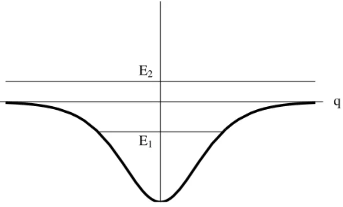
where T(E) is the classical time for the bound motion at energy E (e.g., the energyE1 in figure 5.2).
If the energy is such that the motion is not bound (likeE2in figure 5.2), the timeT(E)is infinite. We can however define the change of level density with respect to a free particle. From (5.10) and the trace formula, we have nfree(E) = mL/⇡¯hp where Lis the volume (length) of the system. We can thus write
n(E) = n0(E) nfree(E)
= m
⇡¯h
Z
dq
0
@ 1
q2m(E V(q)) p 1
2mE
1 A
The advantage of this formula is that its integrand goes to zero in the asymptotic regionq ! 1 where the potential is zero. For energies above bound states, this is the only correction to the level density since there are no finite closed loops.
q E1
E2
Figure 5.2: One-dimensional potential well. No closed loops forE2, closed loops forE1.
For comparison, we calculate the contribution of zero-length loops in D= 3. Using the GREENfunction (5.9), we have
n0(E) = 2m 4⇡2¯h2 lim
q!0Im
Z
RId3qexp ip(q) q/¯h q
= 4⇡m
(2⇡¯h)3
Z
RId3q p(q)
This result may be compared to the standard ‘recipe’ of statistical mechanics
‘Each quantum state occupies a phase space volume equal tohD = (2⇡¯h)D’.
This rule gives
n(E) = 1 (2⇡¯h)3
Z
d3q
Z
d3p (H(p, q) E)
= 1
(2⇡¯h)3
Z
d3q
Z
d3p @p
@E (p p(q;E))
= 4⇡m
(2⇡¯h)3
Z
RId3q p(q;E)
using@p/@E =m/pand spherical coordinates for the momentum integral.
We thus get the zero-length level densityn0(E).
Nontrivial closed loops
Let us call their contribution np(E). Evaluating the integral over q in the trace formula in the stationary phase approximation, we find a stationary point at
0 = @S(q, q;E)
@q = @S
@qB q + @S
@qA q =pB pA
This gives a particular closed loop starting and ending at q with the same momentum,i.e., a periodic trajectoryor periodic orbit. GUTZWILLER’s trace formula thus links the energy level density to a sum over the periodic orbits of the classical system.
‘It has long been known that the periodic orbits are of funda- mental importance in semiclassical mechanics (Einstein 1917, Brillouin 1926, Keller 1958), but their precise meaning is only now becoming clear as a result of this work of Gutzwiller (1971).’
(Berry & Mount, 1972, p.388) The action for a single circuit around a closed orbit (in the positive sense) is
S1(E) = 2
Z q2
q1
dq0p(q0), q1,2 : turning points
We note that it is independent of the particular pointq on the orbit.
For the density Cr along the orbit, we need second derivatives of the action. To start with, we distinguish between starting and end point and
get for the pathqA !q2 !q1 !qB (nearly one return) S(qB, qA;E) =
Z q2
qA
dq0p(q0) +S1(E) +
Z qB q1
dq p(q0) The differentiation gives
@2S
@qB@qA
= @p(qA)
@qB
+ @p(qB)
@qA
= 0 + 0 = 0
because the positions qA,B are independent variables. We must have for- gotten something. . .
This second derivative appeared in the time-dependent propagator, when we related changes of final positions and initial momenta:@pA/@qB =
@2R(B, A)/@qB@qA. There, the time t was kept constant, while here, we deal with the energy-dependent action S(qB, qA;E). Gutzwiller (1990) re- marks that one has to vary both positionand energy:
@pA
@qB t = @pA
@qB E+ @pA
@E q
B
@E
@qB, (5.12)
while the derivative @E/@qB is fixed by the constraint that the time t =
@S/@E =const.. The differentiation of this relation gives 0 = @t
@qB
= @2S
@E@qB
+ @2S
@E2
@E
@qB
.
Putting that into (5.12), we find the ‘transformation matrix on the energy surface’ (Gutzwiller, 1990)
Cij = @pA
@qB t = @2S
@qA@qB + @2S
@qA@E
@2S
@qB@E
@2S
@E2
! 1
(5.13) The (squared) amplitude of the GREENfunction (5.8) thus becomes
@2S
@E2 det(Cij) =
@2S
@E2
!1 D
det @2S
@qA@qB
@2S
@E2 + @2S
@qA@E
@2S
@qB@E
!
InD= 1, the determinant is trivial. We already found that the first term in parentheses vanishes. The second term is found from
@2S
@qB@E = @pB
@E = @
@E
q2m(E V(qB)) = m pB
and a similar result involving m/pA. This result is independent of the number of periods needed to reachqB.
One dimension: BOHR–SOMMERFELD quantisation
We can now letqB !qA and find the level density nr(E)for an orbit with r 2Z\{0}returns
nr(E) = m
⇡¯hRe
Z q2
q1
dq
|p(q)|exp i [rS1(E)/¯h r⇡]
Two phase jumps of ⇡/2 at the turning points are included for each pe- riod. We observe that the result (5.11) for the zero length loops may be recovered by putting r = 0. Furthermore, the one-loop action S1(E)is in- dependent ofq, and the integration gives one half classical period. The full semiclassical level density is therefore
n(E) = n0(E) +np(E)
= T(E) 2⇡¯h
X
r2Z
exp ir[S1(E)/¯h ⇡]
This sum may be evaluated with the help of the POISSON summation for-
mula X
r2Z
eirw = 2⇡ X
n2Z
(w 2⇡n) We thus find
n(E) = T(E)
¯ h
X
n2Z
[S1(E)/¯h ⇡ 2⇡n]
= T(E)X
n 0
[S1(E) (2n+ 1)⇡¯h]
= X
n 0
(E En)
This is a series of -peaks with the energy eigenvalues En given by the BOHR–SOMMERFELD quantisation rule:2
S1(En) = (n+12)2⇡¯h
In the semiclassical regime, the spacing between the energy levels is equal to the inverse classical period:
2⇡¯h= E@S1
@E =) E = 2⇡¯h T(E)
2The transformation of the -function makes use of the relation@S1/@E=T(E).
A large period therefore corresponds to an increased density of the energy levels. For the hydrogen atom, e.g., the period approaches infinity forE % 0; and the spectrum shows indeed an accumulation of levels there.
Finally, if the discrete levels are too close together to be resolved, one gets an ‘averaged’ level density with a value (one state per level spacing)
n(E) = 1
E = T(E)
2⇡¯h =n0(E) This is precisely the contribution of zero-length orbits.
5.5 The spectrum of classically chaotic systems with isolated periodic orbits
In integrable or separable systems, periodic orbits occur in families and cover some part of the coordinate space. This leads to a discrete spectrum.
The more generic case is a non-integrable system. Periodic orbits are then isolated in space. They contribute distinctive features to the energy spectrum that are superimposed on a smooth background (the contribution of the zero length paths).
Classical stability analysis
We introduce a local coordinate system q = (q0, q1, q2)with q1,2 = 0 along on the periodic orbit. If we take a point q¯on the periodic orbit, then the actionS1(q, q;E)for a single circuit along the periodic orbit is independent of q¯0, similar to the one-dimensional case. A trajectory starting with ini- tial position qA and momentum pA slightly offset from a point q,¯ p¯on the periodic orbit will hopefully stay in the vicinity of the orbit and end up at a final position (qB, pB) slightly offset from q,¯ p. The action of this path is¯ given by S(qB, qA;E). To first order in the displacements qA,B =qA,B q,¯ we have
pAi = @2S
@qAi@qAj
qAj
@2S
@qAi@qBj
qBj
pBi = @2S
@qBi@qAj qAj+ @2S
@qBi@qBj qBj
with indices i, j = 1,2. All derivatives are evaluated along the periodic orbit. Gutzwiller (1990) writes this linear system in the abbreviated form
pA = a qA b qB pB = bT qA+c qB
with real2⇥2matricesa, b, ccontaining the second derivatives of the action (bT is the transpose ofb).
A more geometric interpretation of what happens in the vicinity of the periodic orbit is provided by the relation between initial and final devia- tions. This is also a linear system with the matrices
qB = A qA+B pA
pB = C qA+D pA
It is an easy calculation that these matrices are given by A= b 1a B = b 1 C =bT cb 1a D= cb 1
provided the matrixb (with the mixed second derivatives) is nonsingular.
Let us consider the eigenvalues of this linear transformation that may loosely be associated with the LYAPUNOV exponents of the dynamics in phase space. (A more precise definition will be introduced below.) The characteristic polynomial of the linear transformation is (1 is the 2⇥ 2 identity matrix)
F( ) = det
0
@ A 1 B
C D 1
1
A (5.14)
= det
0
@ b 1a 1 b 1 bT cb 1a cb 1 1
1 A
To simplify this determinant, we subtract from the second row the first one, multiplied with c. Furthermore, factoring out b 1 from the first row
and expanding the determinant along the first row, we find F( ) = det
0
@ b 1a 1 b 1 bT + c 1
1
A (5.15)
= 1
det(b)det⇣ a+ 2b+bT + c⌘ (5.16) From this expression, we can read off thatF(0) = 1,i.e., the linear transfor- mation between qA, pA and qB, pB preserves the volume of phase space (LIOUVILLE’s theorem). Furthermore, since the characteristic polynomial F( )is real (the matricesa, b, c being real), the eigenvalues are either real or complex conjugate pairs. Finally, one can also check that whenever is a solution of F( ) = 0, then this is also true for1/ .
The following cases are now distinguished by Gutzwiller (1990):
elliptic orbit: the eigenvalues are pure phase factors = ei ,e i ; (direct) hyperbolic orbit:3 the eigenvalues are real = e ,e ; loxodromic orbit: the eigenvalues are = e±u±iv with realu, v.
For each degree of freedom transverse to the orbit, one gets a pair of eigen- values. We see that loxodromic orbits occur only with three degrees of freedom at least.
The geometric meaning of these cases is the following:
elliptic orbit: the phase space volume is rotated after one circuit along the orbit, but its aspect ratio is preserved. The angle describes the rotation angle per roundtrip. An elliptic periodic orbit is also called
‘stable’ because in the long time limit, neighbouring points remain at a finite distance from the orbit.
hyperbolic orbit: one direction in phase space gets stretched by a factor e , while the other one is shrunk by the opposite factor e . In this context, the quantity may be identified with the LYAPUNOVexponent for the stretched direction. A hyperbolic orbit is also called ‘unstable’
because the distance from the orbit increases without limits in the direction corresponding to the positive LYAPUNOV exponent .
3Inverse hyperbolic orbitshave eigenvalues = e , e .
An elliptic orbit with = 0,⇡ is called a parabolic orbit: in this case, a small cube in phase space is mapped onto itself (or its reflected image) without rotation nor distortion. This case is typical for an integrable system according to GUTZWILLER, but it is non-generic.
Contribution to the level density
After these preparations for the classical dynamics, we can face the contri- bution of a periodic orbit to the quantum-mechanical level density:
n(E) = Im 2
(2⇡i¯h)D+12 ⇥ (5.17)
⇥Z dqX
r
"
@2Sr
@E2Cr
#1/2
exp i [Sr(q, q;E)/¯h µr⇡/2]
We have to integrate over the points q on closed orbits. In the hope that the positions q¯along the periodic orbit will give a dominant contribution, the action Sr(q, q;E)will be expanded in the vicinity of this particular or- bit. For points q¯on the orbit, the action gives a value Sr(E) = Sr(¯q,q;¯ E) independent ofq.¯
The variation to first order in q = q q¯is zero because the orbit is closed: initialpA = @Sr/@qAand final momentapB =@Sr/@qBare equal.
We now use the local coordinate system centred on the orbit introduced above and consider a point displaced by q = q q¯transverse to the or- bit (only the 1,2 components are nonzero). To second order, this gives a variation of the action
Sr = 1 2
@2S
@qAi@qAj
+ 2 @2S
@qAi@qBj
+ @2S
@qBi@qBj
!
qi qj where all derivatives are calculated at the pointq¯on the periodic orbit.
We consider first a single roundtrip around the orbit. Then we can use the matrices a, b, c introduced before and express the second variation of the action as
S1 = 1
2 q·⇣a+b+bT +c⌘· q (5.18) Here, we wrote the matrices in a symmetrised form since this is appropriate for the quadratic form S1. The integration with respect to q (or, equiva- lently, q) is now a multi-(D 1)-dimensional FRESNEL integral, since the
phase S1/¯h is a quadratic form of the displacements q. We neglect the variation of the amplitude factor transverse to the orbit and get
Z
d2qeiS1/¯h = (2⇡i¯h)D21
det (a+b+bT +c)1/2 (5.19) If the (symmetric) matrixa+b+bT +chas a number µof negative eigen- values, then the square root is resolved by taking the absolute value and adding a phase factor e iµ⇡/2. We observe that the determinant in (5.19) also appears in the characteristic polynomialF( )defined in (5.14). More precisely, we have
det⇣a+b+bT +c⌘=F(1) det(b) = F(1) det @2S
@qAi@qBj
!
.
Finally, we have to work out the amplitude factor in the GREENfunction in the trace formula (5.20). From (5.13), we know that the density Cr is a determinant containing second derivatives of the action with respect to position (like the matrices a, b, cand mixed derivates. These may be calcu- lated by differentiating the time-independent HAMILTON–JACOBIequation:
H @S
@qB
, qB
!
=E
In the local coordinate system along the periodic orbit, the differentiation with respect to the (initial) coordinateqAgives (with indices↵, = 0,1,2)
@H
@pB↵
@2S
@qB↵@qA
= 0
This already shows that the full matrix with the mixed derivatives of the action is singular, because the velocity vector vB↵ = @H/@pB↵ is mapped onto zero. Furthermore, in the local coordinates, we know that the velocity points in the 0-direction: vB↵ = (|vB|,0,0). We thus conclude that the elements with↵= 0 of the matrix@2S/@qB↵@qA vanish.
Finally, knowing the momentum pB↵ = @S/@qB↵, we find by taking the derivative with respect to the energyE
@2S
@qB↵@E = m
|pB| ↵,0
The second matrix appearing in (5.13) therefore has only a single nonzero element at the0,0position.
We can now expand the determinant Cr (5.13) with respect to the first row and find
@2S
@E2 det(C↵ )
= @2S
@E2
!1 D
det
0 BB
@
m2/|pA| |pB| 0 0 C10
C20
@2S
@E2
@2S
@qAi@qBj
1 CC A
= ( 1)D 1 m2
|pA| |pB|det @2S
@qAi@qBj
!
where theCj0 are irrelevant matrix elements. We note again that this result is independent of the number of round trips. For a single passage along the periodic orbit, we recover the determinant of the matrix b:
@2S
@E2 det(C↵ ) = ( 1)D 1 m2
|pA| |pB|det(b)
Putting everything together, we find the following expression for the contribution of a single passage (in the positive sense) of the periodic orbit:
n1(E) = Imei[S1(E)/¯h µ1⇡/2]
⇡i¯h
Z
d¯q0
m
|p(¯q0)|
q 1
( 1)D 1F(1) (5.20) Gutzwiller (1990) mentions in passing that F(1) is independent of q¯0 and takes it outside the integral. We are then left with the integration ofd¯q0/¯v that gives the periodT(E)for a single roundtrip along the orbit (the ‘prim- itive period’).
The function F(1)may be calculated from the knowledge of the eigen- values of the phase-space mapping along the orbit. For each degree of free- dom transverse to the orbit, we get a pair of eigenvalues . The discussion is most simple withD= 2. Then a single eigenvalue pair ,1/ is sufficient to characterise the stability of the orbit. The characteristic polynomialF(1) is calculated from
F(1) = (1 )⇣1 1⌘
= 2 ⇣ + 1⌘
For the elliptic and hyperbolic orbits introduced above, we thus find4 elliptic: F(1) = 2 (1 cos ) = 4 sin2( /2) (direct) hyperbolic: F(1) = 2 (1 cosh ) = 4 sinh2( /2) For an elliptic orbit, we thus have
n1(E) = ImT(E) 2⇡¯h
eiw sin( /2)
withw =S1(E)/¯h µ1⇡/2. A similar result holds for the hyperbolic orbit.
Note that this expression does not hold for an integrable system (parabolic orbit with = 0).
Stable orbit: sharp energy levels
What is the contribution of multiple roundtrips of the orbit? The action and the MASLOV index get multiplied by r, the number of roundtrips. The phase-space mapping is the r’th iteration of a single circuit mapping, and therefore its eigenvalues are r. The quantity (in the exponent of ) therefore gets replaced by r . The sum over multiple roundtrips along an elliptic orbit therefore is
ne.o.(E) = ImT(E) 2⇡¯h
X1 r=1
eirw sin(r /2) To compute the sum, we make the expansion
1
sin(r /2) = 2ie ir /2
X1 l=0
e ilr
This expansion is made to converge when we add a negative imaginary part to the stability angle . For each term of the sum overl we now get a geometric series. Its summation gives
ne.o.(E) = ImiT(E)
⇡¯h
X1 l=0
1
e i[w (2l+1) /2] 1
4For an inverse hyperbolic orbit:F(1) = 4 cosh2( /2).
This expression has a pole whenever w (2l+ 1) /2 is a multiple of 2⇡.
Knowing that has a negative imaginary part, we find the following ex- pansion around the poles
1
e i[w (2l+1) /2] 1 = X
n2Z
1
i[w (2l+ 1) /2 2⇡n]
= X
n2Z
✓
⇡ [w (2l+ 1) /2 2⇡n] +
+ iP 1
w (2l+ 1) /2 2⇡n
◆
The level density is now determined by the -function, and we get ne.o.(E) = X
n,l 0
(E En,l)
with S1(En,l) = h(n+ µ41)2⇡+ (l+12) i¯h (5.21) The (stable) elliptic orbit hence leads to a series of sharp, discrete energy eigenvalues that are characterised by two quantum numbers n and l. The quantum number n is analogous to what we saw in one dimension. The
‘stability angle’ may be seen as a correction to phase jump µ1⇡/2 asso- ciated with the MASLOV index. Finally, to interpret the quantum number l, we may speculate that the neighbourhood of the stable periodic orbit is
‘bound’ to it as in a harmonic potential well (this is clear if we linearise the equations of motion around the orbit, for example). The harmonic well contributes a transverse energy (l + 12)¯h! to the eigenvalues. From the quantisation rule (5.21), we read off that!= /T(En,l).
Unstable orbit: resonances
Finally, what changes when the orbit is hyperbolic, i.e., unstable? The contribution of anr-fold roundtrip is found by a similar reasoning to be
nr(E) = ImT(E) 2⇡i¯h
eirw sinh(r /2)
To sum this over the number of roundtrips r, we observe that the distinct features in the level density arise from the behaviour for largerin the sum.
In this regime, we may replace the sinh( /2)by its asymptotic form 12e /2.
The sum then becomes again a geometric series, but in distinction to the stable orbit, we get denominators with a resonant behaviour (without poles for realw):
1
e iw+ /2 1 = iX
n2Z
w 2⇡n i /2 (w 2⇡n)2+ 2/4
This expansion in the vicinity of the poles is valid when the dimensionless actionwis much larger than the LYAPUNOVexponent and when is small compared to unity.
The energy spectrum thus shows a series of lorentzian resonances:
nh.o.(E) = T(E) 2⇡
X
n 0
¯ h
(S1(E) (n+ µ41)2⇡¯h)2+ ¯h2 2/4 (5.22) The resonances are centered at the energies En from the BOHR– SOMMERFELD quantisation rule:
S1(En) = (n+µ41)2⇡¯h
Their widthh¯ nis related to the LYAPUNOV exponent by
¯
h n ⇡ ¯h T(En)
The periodic unstable orbit thus leads to a series of resonances in the en- ergy range where the orbit exists. Their spacing is given by ¯h/T(E). The resonances may be individually resolved if the LYAPUNOV exponent (that determines their width) is much smaller than unity, i.e., if the orbit is not too unstable.
Bibliography
M. V. Berry & K. E. Mount (1972). Semiclassical approximations in wave mechanics,Rep. Prog. Phys. 35, 315–397.
M. C. Gutzwiller (1971). Periodic orbits and classical quantization condi- tions,J. Math. Phys.12(3), 343–58.
M. C. Gutzwiller (1990). Chaos in Classical and Quantum Mechanics. vol- ume 1 ofInterdisciplinary Applied Mathematics. Springer, New York.