Normal modes

1. double slit experiment with electrons of Tonomura 2. photons on photo plate,

3. many-body dynamics in ultracold atom experiments in optical lattices Possible configurations are particularly evident in the case of fermionic atoms (assuming spin s = 1/2, for simplicity) in optical lattices. Due to the Pauli principle each lattice site can be occupied only by zero, one or two atoms – in the latter case they have to have different spin projections. If an initial config- uration of atoms is excited (e.g. by a confinement quench), a dynamical evo- lution will start. This will, of course, not be described by the time-dependent Schr¨odinger equation for the many-atom wave function! This equation only describes the average dynamics that follow from averaging over the dynamics that start from many independent realizations. This has been very successful but, on the other hand, reproduces only part of the information. For exam- ple, it completely misses the fluctuations of the numbers of atoms around the average.⁷

“First” quantization is evident in the case of particle motion in a confining potentialU(r), such as an oscillator potential: classical bounded motion trans- forms, in quantum mechanics, into a set of eigenstates|ψ_ni(that are localized as well) that exist only for a sequence of discrete (quantized) energiesE_n. This example is discussed more in detail below.

2.3 The linear harmonic oscillator and the lad- der operators

Let us now recall the simplest example of quantum mechanics: one particle in a one-dimensional harmonic potentialU(x) = ^m₂ω²x², i.e. in Eq. (2.1),N = 1 and the interaction potentials vanish. We will use this example to introduce the basic idea of “second quantization”. In writing the potential U(x) we switched to the coordinate representation where states|ψ_niare represented by functions of the coordinate, ψ_n(x). At the end we will return to the abstract notation in terms of Dirac states.

7This section is not complete yet.

2.3.1 One-dimensional harmonic oscillator

The stationary properties of the harmonic oscillator follow from the stationary Schr¨odinger equation (2.28) which now becomes, in coordinate representation

H(ˆˆ x,p)ψˆ _n(x) = pˆ²

2m + mω² 2 xˆ²

ψ_n(x) =E_nψ_n(x), (2.29) where ˆx = x and ˆp = ^~_idx^d . We may bring the Hamilton operator to a more symmetric form by introducing the dimensionless coordinate ξ = x/x₀ with the length scale x₀ = [~/mω]^1/2, whereas energies will be measured in units of

~ω. Then we can replace _dx^d = _x¹

0

d

dξ and obtain Hˆ

~ω = 1 2

− ∂²

∂ξ² +ξ²

. (2.30)

This quadratic form can be rewritten in terms of a product of two first order operators a, a^†, the “ladder operators”,

a = 1

√2 ∂

∂ξ +ξ

, (2.31)

a^† = 1

√2

−∂

∂ξ +ξ

. (2.32)

Indeed, computing the product Nˆ = a^†a= 1

√2 ∂

∂ξ +ξ 1

√2

− ∂

∂ξ +ξ

(2.33)

= 1

2

−∂²

∂ξ² +ξ²−1

,

the hamiltonian (2.30) can be written as Hˆ

~ω = ˆN + 1

2. (2.34)

It is obvious from (2.34) that ˆN commutes with the hamiltonian,

[ ˆH,Nˆ] = 0, (2.35)

and thus the two have common eigenstates. This way we have transformed the hamiltonian from a function of the two non-commuting hermitean operators

ˆ

x and ˆp into a function of the two operators a and a^† which are also non- commuting⁸, but not hermitean, instead they are the hermitean conjugate of each other,

[a, a^†] = 1, (2.36)

(a)^† = a^†, (2.37)

which is easily verified.

The advantage of the ladder operators is that they allow for a straight- forward computation of the energy spectrum of ˆH, using only the properties (2.33) and (2.36), without need to solve the Schr¨odinger equation, i.e. avoid- ing explicit computation of the eigenfunctions ψ_n(ξ) ⁹. This allows us to re- turn to a representation-independent notation for the eigenstates, ψ_n → |ni. The only thing we require is that these states are complete and orthonormal, ˆ1 =P

n|nihn|and hn|n^′i=δ_n,n′.

Now, acting with ˆN on an eigenstate, using Eq. (2.34), we obtain Nˆ|ni=a^†a|ni =

E_n

~ω −1 2

|ni=n|ni, ∀n, (2.38) n = E_n

~ω − 1 2,

where the last line relates the eigenvalues of ˆN and ˆn that correspond to the common eigenstate|ni. Let us now introduce two new states that are created by the action of the ladder operators,

a|ni = |n˜i, a^†|ni = |n¯i,

where this action is easily computed. In fact, multiplying Eq. (2.38) from the left bya, we obtain

aa^†|n˜i= E_n

~ω −1 2

|n˜i.

Using the commutation relation (2.36) this expression becomes a^†a|n˜i=

E_n

~ω −3 2

|n˜i= (n−1)|n˜i,

8The appearance of the standard commutator indicates that these operators describe bosonic excitations.

9We will use the previous notation ψ, which means that the normalization is x0R

dξ|ψ(ξ)|²=1

which means the state|n˜iis an eigenstate of ˆN [and, therefore, of ˆH] and has an energy lower than|niby~ωwhereas the eigenvalue of ˆN is ˜n=n−1. Thus, the action of the operator a is to switch from an eigen state with eigenvalue n to one with eigenvalue n−1. Obviously, this is impossible for the ground state, i.e. when aacts on |0i, so we have to require

|˜0i=a|0i ≡0. (2.39)

When we use this result in Eq. (2.38) forn= 0, the l.h.s. is zero with the con- sequence that the term in parantheses must vanish. This immediately leads to the well-known result for the ground state energy: E₀ =~ω/2, corresponding to the eigenvalue 0 of ˆN.

From this we now obtain the energy spectrum of the excited states: acting witha^† from the left on Eq. (2.38) and using the commutation relation (2.36), we obtain

Nˆ|n¯i= E_n

~ω −1 2+ 1

|n¯i= ¯n|n¯i.

Thus, ¯n is again an eigenstate of ˆN and ˆH. Further, if the eigenstate |ni has an energy E_n, cf. Eq. (2.38), then ¯n has an energy E_n +~ω, whereas the associated eigenvalue of ˆN is ¯n = n+ 1. Starting from the ground state and acting repeatedly witha^† we construct the whole spectrum,E_n, and may express all eigenfunctions via ψ₀:

E_n = ~ω

n+ 1 2

, n= 0,1,2, . . . (2.40)

|ni = C_n a^†n

|0i. (2.41)

C_n = 1

√n!, (2.42)

where the normalization constant C_n will be verified from the properties of a^† below. The above result shows that the eigenvalue of the operator ˆN is just the quantum number n associated with the eigenstate |ni. In other words, since

|ni is obtained by applyinga^† to the ground state function n times or by “n- fold excitation”, the operator ˆN is the number operator counting the number of excitations (above the ground state). Therefore, if we are not interested in the analytical details of the eigenstates we may use the operator ˆN to count the number of excitations “contained” in the system. For this reason, the common notion for the operator a(a^†) is “annihilation” (“creation”) operator of an excitation. For an illustration, see Fig. 2.3.1.

Figure 2.1: Left: oscillator potential and energy spectrum. The action of the operators a and a^† is illustrated. Right: alternative interpretation: the op- erators transform between “many-particle” states containing different number of elementary excitations.

From the eigenvalue problem of ˆN, Eq. (2.38) we may also obtain the explicit action of the two operatorsa and a^†. Since the operator atransforms a state into one with quantum number n lower by 1 we have

a|ni=√

n|n−1i, n= 0,1,2, . . . (2.43) where the prefactor may be understood as an ansatz¹⁰. The correctness is proven by deriving, from Eq. (2.43), the action of a^† and then verifying that we recover the eigenvalue problem of ˆN, Eq. (2.38). The action of the creation operator is readily obtained using the property (2.37):

a^†|ni = X

¯ n

|¯nihn¯|a^†|ni=X

¯ n

|n¯ia[h¯n|]|ni

= X

¯ n

|¯ni√

¯

nhn¯−1|ni= √

n+ 1|n+ 1i. (2.44) Inserting these explicit results for a and a^† into Eq. (2.38), we immediately verify the consistency of the choice (2.43). Obviously the oscillator eigenstates

|niare no eigenstates of the creation and annihilation operators ¹¹. Problems:

1. Calculate the explicit form of the ground state wave function by using Eq. (2.39).

2. Show that the matrix elements ofa^† are given by

n+ 1|a^†|n

=√ n+ 1, where n= 0,1, . . ., and are zero otherwise.

3. Show that the matrix elements ofaare given byhn−1|a|ni=√n, where n= 0,1, . . ., and are zero otherwise.

4. Proof relation (2.42).

10This expression is valid also forn= 0 where the prefactor assures that application ofa to the ground state does not lead to a contradiction.

11A particular case are Glauber states (coherent states) that are a special superposition of the oscillator states which are the eigenstate of the operatora.

2.3.2 Generalization to several uncoupled oscillators

The previous results are directly generalized to a three-dimensional harmonic oscillator with frequenciesω_i, i = 1,2,3, which is described by the hamiltonian

Hˆ =

3

X

i=1

H(ˆˆ x_i,pˆ_i), (2.45)

which is the sum of three one-dimensional hamiltonians (2.29) with the po- tential energy U(x₁, x₂, x₃) = ^m₂(ω²₁x²₁ +ω₂²x²₂ + ω²₃x²₃). Since [p_i, x_k] ∼ δ_k,i all three hamiltonians commute and have joint eigenfunction (product states).

The problem reduces to a superposition of three independent one-dimensional oscillators. Thus we may introduce ladder operators for each component inde- pendently as in the 1d case before,

a_i = 1

√2 ∂

∂ξ_i +ξ_i

, (2.46)

a^†_i = 1

√2

− ∂

∂ξ_i +ξ_i

, [a_i, a^†_k] =δ_i,k. (2.47) Thus the hamiltonian and its eigenfunctions and eigenvalues can be written as

Hˆ =

3

X

i=1

~ω_i

a^†_ia_i+ 1 2

a_i|0i = 0, i= 1,2,3 ψ_n1,n2,n3 =|n₁n₂n₃i = 1

√n₁!n₂!n₃!(a^†₁)ⁿ¹(a^†₂)ⁿ²(a^†₃)ⁿ³|0i (2.48)

E =

3

X

i=1

~ω_i

n_i+ 1 2

.

Here |0i ≡ |000i = |0i|0i|0i denotes the ground state and a general state

|n1n2n3i =|n1i|n2i|n3i contains ni elementary excitations in direction i, cre- ated by n_i times applying operator a^†_i to the ground state.

Finally, we may consider a more general situation of any number M of coupled independent linear oscillators and generalize all results by replacing the dimension 3→M.

Figure 2.2: Illustration of the one-dimensional chain with nearest neighbor interaction. The chain is made infinite by connecting particle N + 1 with particle 1 (periodic boundary conditions).

2.4 Generalization to interacting particles.

Normal modes

The previous examples of independent linear harmonic oscillators are of course the simplest situations which, however, are of limited interest. In most prob- lems of many-particle physics the interaction between the particles which was neglected so far, is of crucial importance. We now discuss how to apply the formalism of the creation and annihilation operators to interacting systems.

2.4.1 One-dimensional chain and its normal modes

We consider the simplest case of an interacting many-particle system: N iden- tical classical particles arranged in a linear chain and interacting with their left and right neighbor via springs with constantk.¹², see Fig. 2.2.

This is the simplest model of interacting particles because each particle is assumed to be fixed around a certain positionx_i in space around which it can perform oscillations with the displacement q_i and the associated momentum p_i.¹³ Then the hamiltonian (2.1) becomes

H(p, q) =

N

X

j=1

p²_j 2m + k

2(q_j−q_j+1)²

. (2.49)

Applying Hamilton’s equations we obtain the system of equations of motion (2.4)

mq¨_j =k(q_j+1−2q_j +q_j−1), j = 1. . . N (2.50) which have to be supplemented with boundary and initial conditions. In the following we consider a macroscopic system and will not be interested in ef- fects of the left and right boundary. This can be achieved by using “peri- odic” boundary conditions, i.e. periodically repeating the system according to

12Here we follow the discussion of Huang [Hua98].

13Such “lattice” models are very popular in theoretical physics because they allow to study many-body effects in the most simple way. Examples include the Ising model, the Anderson model or the Hubbard model of condensed matter physics.

Figure 2.3: Dispersion of the normal modes, Eq. (2.53), of the 1d chain with periodic boundary conditions.

q_j+N(t) =q_j(t) for allj [for solutions for the case of a finite system, see Prob- lem 5]. We start with looking for particular (real) solutions of the following form¹⁴

q_j(t) =e^i(−ωt+jl)+c.c., (2.51) which, inserted into the equation of motion, yield for any j

−mω² q_j+q^∗_j

=k e^il−2 +e^−il

q_j+q_j^∗

, (2.52)

resulting in the following relation between ω and k (dispersion relation)¹⁵: ω²(l) =ω²₀sin² l

2, ω₀² = 4k

m. (2.53)

Hereω₀is just the eigenfrequency of a spring with constantk, and the prefactor 2 arises from the fact that each particle interacts with two neighbors. While the condition (2.53) is independent of the amplitudes q_j⁰, i.e. of the initial conditions, we still need to account for the boundary (periodicity) condition.

Inserting it into the solution (2.51) gives the following condition forl, indepen- dently of ω: l → l_n = _Nⁿ2π, where n = 0,±1,±2,· · · ± ^N₂. Thus there exists a discrete spectrum ofN frequencies of modes which can propagate along the chain (we have to exclude n= 0 since this corresponds to a time-independent trivial constant displacement),

ω²_n = 4k

msin²nπ

N, n=±1,±2,· · · ±N

2. (2.54)

This spectrum is shown in Fig. 2.3. TheseN solutions are the complete set of normal modes of the system (2.49), corresponding to itsN degrees of freedom.

These are collective modes in which all particles participate – all oscillate with the same frequency but with a well-defined phase which depends on the particle number. These normal modes are waves running along the chain with a phase velocity¹⁶ c_n ∼ω_n/l_n.

14In principle, we could use a prefactor q⁰_j = q⁰ different from one, but by rescaling of q it can always be eliminated. The key is that the amplitudes of all particles are strictly coupled.

15We use the relation 1−cosx= 2 sin^2x₂.

16The actual phase velocity isωn/kn, where the wave numberkn=ln/ainvolves a length scaleawhich does not appear in the present discrete model.

Due to the completeness of the system of normal modes, we can expand any excitation of particlej and the corresponding momentum, p_j(t) =mq˙_j(t), into a superposition of normal mode contributions (n6= 0)

q_j(t) = 1

√N

N 2

X

n=−^N₂

Q⁰_neⁱ(^−ωnt+2πNⁿj) = 1√ N

N 2

X

n=−^N₂

e^−iωntQ_n(j), (2.55)

p_j(t) = 1

√N

N 2

X

n=−^N₂

P_n⁰eⁱ(^−ωnt+2π_N^nj) = 1√ N

N 2

X

n=−^N₂

e^−iωntP_n(j), (2.56)

whereP_n⁰ =−imω_nQ⁰_n. Note that the complex conjugate contribution to mode n is contained in the sum (term−n). Also, q_j(t) and p_j(t) are real functions.

By computing the complex conjugateq_j^∗and equating the result toq_jwe obtain the conditions (Q⁰_n)^∗ =Q⁰_−n and ω_−n =−ω_−n. Analogously we obtain for the momenta (P_n⁰)^∗ = P_−n⁰ . To make the notation more compact we introduced the N-dimensional complex vectors Q~_n and P~_n with the component j being equal to Q_n(j) = Q⁰_ne^i2πnj/N and P_n(j) = P_n⁰e^i2πnj/N. One readily proofs¹⁷ that these vectors form an orthogonal system by computing the scalar product (see problem 5)

Q~_nQ~_m =Q⁰_nQ⁰_m

N

X

j=1

e^{i2πn+mN j} =N Q⁰_nQ⁰_mδ_n,−m. (2.57)

Using this property it is now straightforward to compute the hamilton function in normal mode representation. Consider first the momentum contri- bution,

N

X

j=1

p²_j(t) = 1 N

N 2

X

n=−^N₂

N 2

X

m=−^N₂

P~_nP~_me^{−i(ωn+ωm)t}, (2.58)

where the sum over j has been “absorbed” in the scalar product. Using now the orthogonality condition (2.57) we immediately simplify

N

X

j=1

p²_j(t) =X

n

|P_n⁰|². (2.59)

17See problem 5

Analogously, we compute the potential energy

U = k

2

N

X

j=1

[q_j(t)−q_j+1(t)]² = k 2N

N 2

X

n=−^N₂

N 2

X

m=−^N₂

e^{−i(ωn+ωm)t}

×

N

X

j=1

Q⁰_nQ⁰_m

e^i2πNnj−e^i2πNn(j+1)

e^i2πmNj −e^i2πmN(j+1) .

The sum over j can again be simplified, using the orthogonality condition (2.57), which allows to replace mby −n,

1 N

N

X

j=1

Q⁰_nQ⁰_m

e^i2πNnj−e^i2πNn(j+1)

e^i2πmNj−e^i2πmN(j+1) =

= 1−e^i2πNn

1−e^i2πmNQ~_nQ~_m=

= 2

1−cos2πn N

δ_n,−mQ⁰_nQ⁰_m= 4ω_n²

ω²₀δ_n,−m|Q⁰_n|²,

where we have used Eq. (2.53) and the relation 1−cosx= 2 sin^{2 x}₂. This yields for the potential energy

U = k 2

X

n

mω²_n k

and for the total hamilton function H(P, Q) =

N 2

X

n=−^N₂

1

2m|P_n⁰|²+ m

2ω_n²|Q⁰_n|²

. (2.60)

Problem 5: Prove the orthogonality relation (2.57).

2.4.2 Quantization of the 1d chain

We now quantize the interacting system (2.49) by replacing coordinates and momenta of all particles by operators

(q_i, p_i) → (ˆq_i,pˆ_i), i= 1, . . . N,

with qˆ^†_i = qˆ_j, pˆ^†_i = ˆp_i, [ˆq_i,pˆ_j] =i~δ_ij. (2.61)

The Hamilton function (2.49) now becomes an operator of the same functional form (correspondence principle),

H(ˆˆ p,q) =ˆ

N

X

j=1

pˆ²_j 2m + k

2(ˆq_j−qˆ_j+1)²

,

and we still use the periodic boundary conditions ˆq_N+i = ˆq_i. The normal modes of the classical system remain normal modes in the quantum case as well, only the amplitudesQ⁰_n and P_n⁰ become operators

ˆ

q_j(t) = 1

√N

N 2

X

n=−^N₂

e^−iωntQˆ_n(j) (2.62)

p_j(t) = 1

√N

N 2

X

n=−^N₂

e^−iωntPˆ_n(j), (2.63)

where ˆQ_n(j) = ˆQ⁰_nexp{i2πnj/N}, ˆP_n(j) = ˆP_n⁰exp{i2πnj/N} and ˆP_n⁰ =

−imω_nQˆ⁰_n.

What remains is to impose the necessary restrictions on the operators ˆQ⁰_n and ˆP_n⁰ such that they guarantee the properties (2.61). One readily verifies that hermiticity of the operators is fulfilled if ( ˆQ⁰)^†_n = ˆQ⁰_−n, ( ˆP⁰)^†_n = ˆP_−n⁰ and ω_−n = −ω_n. Next, consider the commutator of ˆq_i and ˆp_j and use the normal mode representations (2.62, 2.63),

[ˆq_k,pˆ_j] = 1 N

X

n

X

m

[ ˆQ⁰_n,Pˆ_m⁰]e^{−i(ωn+ωm)t}e^i2πN(kn+jm). (2.64) A sufficient condition for this expression to be equali~δ_k,j is evidently [ ˆQ⁰_n,Pˆ_m⁰] = i~δ_n,−m which is verified separately for the cases k = j and k 6= j. In other words, the normal mode operators obey the commutation relation

hQˆ⁰_n,( ˆP_m⁰)^†i

=i~δ_n,m, (2.65)

and the hamiltonian becomes, in normal mode representation, Hˆ( ˆP ,Q) =ˆ

N 2

X

n=−^N₂

1

2m|Pˆ_n⁰|²+m

2ω²_n|Qˆ⁰_n|²

. (2.66)

This is a superposition ofN independent linear harmonic oscillators with the frequenciesω_n given by Eq. (2.54). Applying the results for the superposition

of oscillators, Sec. 2.3.2, we readily can perform the second quantization by defining dimensionless coordinates, ξ_n = p_mωn

~ Q_n, n = −^N₂, . . .^N₂, n 6= 0, and introducing the creation and annihilation operators,

a_n = 1

√2 ∂

∂ξ_n +ξ_n

, (2.67)

a^†_n = 1

√2

− ∂

∂ξ_n +ξ_n

, [a_n, a^†_k] =δ_n,k. (2.68) Thus the hamiltonian and its eigenfunctions and eigenvalues can be written as

Hˆ =

N 2

X

n=−^N₂

~ω_n

a^†_na_n+ 1 2

a_n|0i = 0, n= −N 2, . . .N

2 ψ_m1,...mN =|m₁. . . m_Ni = 1

√m₁!. . . m_N! a^†

−^N₂

m1

. . . a^†N

2

mN

|0i

E =

N 2

X

n=−^N₂

~ω_n

m_n+ 1 2

.

Here |0i ≡ |0. . .0i = |0i. . .|0i [N factors] denotes the ground state and a general state |m_−N/2. . . m_N/2i = |m_−N/2i. . .|m_N/2i contains m_n elementary excitations of the normal mode n, created by m_n times applying operator a^†_n to the ground state.

Problem 6: The commutation relation (2.65) which was derived to satisfy the commutation relations of coordinates and momenta is that of bosons. This result was independent of whether the particles in the chain are fermions or bosons. Discuss this seeming contradiction.

2.4.3 Generalization to arbitrary interaction

Of course, the simple 1dchain is a model with a limited range of applicability.

A real system ofN interacting particles in 1dwill be more difficult, at least by three issues: first, the pair interaction potentialV may have any form. Second, the interaction, in general, involves not only nearest neighbors, and third, the effect of the full 3d geometry may be relevant. We, therefore, now return to

the general 3d system of N classical particles (2.1) with the total potential energy¹⁸

U_tot(q) =

N

X

i=1

U(r_i) + X

1≤i<j≤N

V(r_i−r_j), (2.69) leading to Newton’s equations

m¨r_i =− ∂

∂r_iU_tot(q), i= 1, . . . N. (2.70) Let us consider stationary solutions, where the time derivatives on the l.h.s.

vanish. The system will then be in a stationary state “s^′′ corresponding to a minimum q⁽⁰⁾s of U_tot of depth Us⁽⁰⁾ = U_tot(q⁽⁰⁾s ) [the classical ground state corresponds to the deepest minimum]. In the case of weak excitations from the minimum,q=q_s⁽⁰⁾+ξ, with|ξ|<< q_s⁽⁰⁾, the potential energy can be expanded in a Taylor series¹⁹

Utot(q) =U_s⁽⁰⁾+ ∂

∂qUtot(q=q⁽⁰⁾_s )ξ + 1

2ξ^TH^(s)ξ+... (2.71) where all first derivatives are zero, and we limit ourselves to the second order (harmonic approximation). Here we introduced the 3N ×3N Hesse matrix Hij^(s) = _∂x^∂2

i∂xjU_tot(q = qs⁽⁰⁾), where x_i, x_j = x₁, y₁, . . . z_N, and ξ^T is the trans- posed vector (row) of ξ. Thus, for weak excitations, the potential energy change ∆U_tot = U_tot(q)−Us⁽⁰⁾ is reduced to an expression which is quadratic in the displacements ξ, i.e. we are dealing with a system of coupled harmonic oscillators²⁰

We can easily transform this to a system of uncoupled oscillators by di- agonalizing the Hesse matrix which can be achieved by solving the eigenvalue problem (we take the mass out for dimensional reasons)

λ_nmQ_n =HQ_n, n= 1, . . .3N. (2.72) Since H is real, symmetric and positive definite²¹ the eigenvalues are real and positive corresponding to the normal mode frequencies ω_n = √

λ_n. Fur- thermore, as a result of the diagonalization, the 3N-dimensional eigenvectors

18Here we follow the discussion of Ref. [HKL⁺09]

19Recall thatq,qs⁽⁰⁾and ξ are 3N-dimensional vectors in configuration space.

20Strictly speaking, from the 3N degrees of freedom, up to three [depending on the sym- metry of U] may correspond to rotations of the whole system (around one of the three coordinate axes, these are center of mass excitations which do not change the particle dis- tance), and the remaining are oscillations.

21qs⁽⁰⁾corresponds to a mininmum, so the local curvature ofUtotis positive in all directions

form a complete orthogonal system {Q_n} with the scalar product Q_nQ_m ≡ P3N

i=1Q_n(i)Q_m(i) ∼ δ_m,n which means that any excitation can be expanded into a superposition of the eigenvectors (normal modes),

q(t) =q⁽⁰⁾_s +

3N

X

n=1

c_n(t)Q_n. (2.73)

The expansion coefficients c_n(t) (scalar functions) are the normal coordinates.

Their equation of motion is readily obtained by inserting a Taylor expansion of the gradient of U_tot [analogous to (2.71)] into (2.70),

0 =mq¨+ ∂U_tot

∂q =m¨q+H ·ξ, (2.74)

and, using Eq. (2.73) for ¨q and eliminatingH with the help of (2.72), 0 =m

3N

X

n=1

¨c_n(t) +c_n(t)ω²_n Q_n. (2.75) Due to the orthogonality of the Q_n which are non-zero, the solution of this equation implies that the terms in the parantheses vanish simultaneously for every n, leading to an equation for a harmonic oscillator with the solution

c_n(t) =A_ncos{ω_nt+B_n}, n= 1, . . .3N, (2.76) where the coefficients A_n and B_n depend on the initial conditions. Thus, the normal coordinates behave as independent linear 1d harmonic oscillators.

In analogy to the coordinates, also the particle momenta, corresponding to some excitation q(t), can be expanded in terms of normal modes by using p(t) = mq(t). Using the result for˙ c_n(t), Eq. (2.76), we have the following general expansion

q(t)−q_s⁽⁰⁾ =

3N

X

n=1

A_ncos{ω_nt+B_n}Q_n ≡

3N

X

n=1

Q_n(t) (2.77) p(t) =

3N

X

n=1

A_nsin{ω_nt+B_n}P_n ≡

3N

X

n=1

P_n(t), (2.78) where the momentum amplitude vector is P_n = −mω_nQ_n. Finally, we can transform the Hamilton function into normal mode representation, using the harmonic expansion (2.71) of the potential energy

H(p, q) = p²

2m +U_tot(q) =U_s⁽⁰⁾+

N

X

i=1

p²_i 2m+ 1

2 X

i6=j

ξ^T(i)Hij^(s)ξ(j). (2.79)

Eliminating the Hesse matrix with the help of (2.72) and inserting the expan- sions (2.77) and (2.78) we obtain

H(p, q)−U_s⁽⁰⁾ =

3N

X

n=1 3N

X

n^′=1

P_n(t)P_n′(t)

2m + m

2ω_n²δ_n,n^′Q_n(t)Q_n^′(t)

=

3N

X

n=1

P_n²(t) 2m + m

2ω_n²Q²_n(t)

≡H(P, Q), (2.80) where, in the last line, the orthogonality of the eigenvectors has been used.

Thus we have succeeded to diagonalize the hamiltonian of the N-particle system with arbitrary interaction. Assuming weak excitations from a station- ary state the hamiltonian can be written as a superposition of 3N normal modes. This means, we can again apply the results from the case of uncou- pled harmonic oscillators, Sec. 2.3.2, and immediately perform the “first” and

“second” quantization.

2.4.4 Quantization of the N -particle system

For the first quantization we have to replace the normal mode coordinates and momenta by operators,

Q_n(t) → Qˆ_n(t) =A_ncos{ω_nt+B_n}Qˆ_n

P_n(t) → Pˆ_n(t) =A_nsin{ω_nt+B_n}Pˆ_n, (2.81) leaving the time-dependence of the classical system unchanged. Further we have to make sure that the standard commutation relations are fulfilled, i.e.

[ ˆQ_n,Pˆ_m] = i~δ_n,m. This should follow from the commutation relations of the original particle coordinates and momenta, [x_iα, p_jβ] = i~δ_i,jδ_α,β, where α, β = 1,2,3 and i, j= 1, . . . N, see Problem 7. Then, the Hamilton operator becomes, in normal mode representation

H( ˆˆ P ,Q) =ˆ

3N

X

n=1

(Pˆ_n²(t) 2m + m

2ω_n²Qˆ²_n(t) )

, (2.82)

which allows us to directly introduce the creation and annihilation operators by introducingξ_n =p_mωn

~ Qˆ_n, n= 1, . . .3N) a_n = 1

√2 ∂

∂ξ_n +ξ_n

, (2.83)

a^†_n = 1

√2

− ∂

∂ξ_n +ξ_n

, [a_n, a^†_k] =δ_n,k. (2.84)

Thus the hamiltonian and its eigenfunctions and eigenvalues can be written as

Hˆ =

3N

X

n=1

~ω_n

a^†_na_n+ 1 2

a_n|0i = 0, n= 1, . . .3N ψ_n1,...n3N = |n₁. . . n_3Ni = 1

√n₁!. . . n_3N!(a^†₁)ⁿ¹. . .(a^†_3N)^n3N|0i

E =

3N

X

n=1

~ω_n

n_n+ 1 2

.

Here |0i ≡ |0. . .0i = |0i. . .|0i [3N factors] denotes the ground state and a general state|n₁. . . n_3Ni=|n₁i. . .|n_3Nicontainsn_n elementary excitations of the normal mode n, created by n_n times applying operator a^†_n to the ground state.

In summary, in finding the normal modes of the interactingN-particle sys- tem the description is reduced to a superposition of independent contributions from 3N degrees of freedom. Depending on the system dimensionality, these include (for a three-dimsional system) 3 translations of the center of mass and 3 rotations of the system as a whole around the coordinate axes. The remaining normal modes correspond to excitations where the particle distances change.

Due to the stability of the stationary state with respect to weak excitations, these relative excitations are harmonic oscillations which have been quantized.

In other words, we have 3N−6 phonon modes associated with the correspond- ing creation and annihilation operators and energy quanta. The frequencies of the modes are determined by the local curvature of the total potential energy (the diagonal elements of the Hesse matrix).

Problem 7: Prove the commutation relation [ ˆQ_n,Pˆ_m] =i~δ_n,m.

Problem 8: Apply the concept of the eigenvalue problem of the Hesse matrix to the solution of the normal modes of the 1dchain. Rederive the normal mode representation of the hamiltonian and check if the time dependencies vanish.

2.5 Continuous systems

2.5.1 Continuum limit of 1d chain

So far we have considered discrete systems containingN point particles. If the number of particles grows and their spacing becomes small we will eventually reach a continuous system – the 1d chain becomes a 1dstring. We start with assigning particle i a coordinatex_j = jawhere j = 0, . . . N, ais the constant interparticle distance and the total length of the system is l=N a, see Fig.

We again consider a macroscopic system which is now periodically repeated after length l, i.e. points x = 0 and x = l are identical²². In the discrete system we have an equally spaced distribution of masses m of point particles with a linear mass density ρ = m/a. The interaction between the masses is characterized by an elastic tension σ = κa where we relabeled the spring constant by κ. The continuum limit is now performed by simulataneously increasing the particle number and reducing a but requiring that the density and the tension remain unchanged,

a, m −→ 0 N, κ −→ ∞ l, ρ, σ = const.

We now consider the central quantity, the displacement of the individual par- ticles q_i(t) which now transforms into a continuous displacement field q(x, t).

Further, with the continuum limit, differences become derivatives and the sum over the particles is replaced by an integral according to

q_j(t) −→ q(x, t) q_j+1−q_j −→ a∂q

∂x X

j

−→ 1 a

Z l

0

dx.

Instead of the Hamilton function (2.49) we now consider the Lagrange function which is the difference of kinetic and potential energy, L = T −V,

22Thus we have formally introducedN+ 1 lattice points but onlyN are different.

Figure 2.4: Illustration of the minimal action principle: the physical equa- tion of motion corresponds to the tractory q(x, t) which minimizes the action, Eq. (2.87) at fixed initial and final points (t_i,0) and (t_f, l).

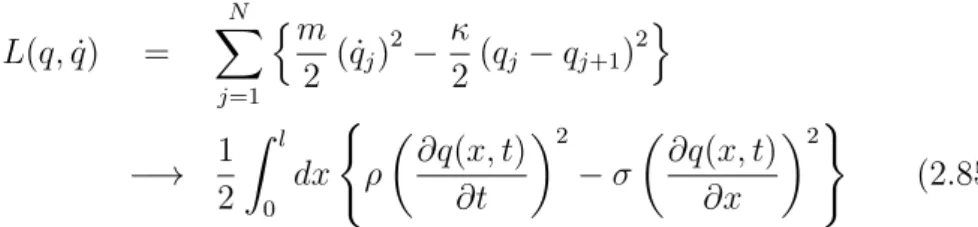
which in the continuum limit transforms to L(q,q)˙ =

N

X

j=1

nm

2 ( ˙q_j)²−κ

2(q_j−q_j+1)²o

−→ 1 2

Z l

0

dx (

ρ

∂q(x, t)

∂t 2

−σ

∂q(x, t)

∂x

2)

(2.85) The advantage of using the Lagrange function which now is a functional of the displacement field, L=L[q(x, t)], is that there exists a very general method of finding the corresponding equations of motion – the minimal action principle.

2.5.2 Equation of motion of the 1d string

We now define the one-dimensional Lagrange density L L=

Z l

0

dxL[ ˙q(x, t), q^′(x, t)], (2.86) where Eq. (2.85) shows that Lagrange density of the spring depends only on two fields – the time derivative ˙q and space derivative q^′ of the displacement field. The action is defined as the time integral of the Lagrange function between a fixed initial time t_i and final time t_f

S = Z tf

ti

dtL= Z tf

ti

dt Z l

0

dxL[ ˙q(x, t), q^′(x, t)]. (2.87) The equation of motion of the 1d string follows from minimizing the action with respect to the independent variables ofL[this “minimal action principle”

has been discussed in detail in Chapter 1, Sec. 1.1], for illustration, see Fig. 2.4,

0 =δS = Z tf

ti

dt Z l

0

dx δL

δq˙δq˙+ δL δq^′δq^′

= Z tf

ti

dt Z l

0

dx {ρq δ˙ q˙−σq^′δq^′}. (2.88)

We now change the order of differentiation and variation,δq˙= _∂t^∂δq and δq^′ =

∂

∂xδq and perform partial integrations with respect to tin the first term and x in the second term of (2.88)

0 =− Z tf

ti

dt Z l

0

dx {ρ¨q −σq^′′} δq, (2.89) where the boundary values vanish because one requires that the variation δq(x, t) are zero at the border of the integration region, δq(0, t) =δq(l, t)≡0.

Since this equation has to be fulfilled for any fluctuation δq(x, t) the term in the parantheses has to vanish which yields the equation of motion of the 1d string

∂²q(x, t)

∂t² −c²∂²q(x, t)

∂x² = 0, with c= rσ

ρ =a rκ

m. (2.90)

This is a linear wave equation for the displacement field, and we introduced the phase velocity, i.e. the sound speed c. The solution of this equation can be written as

q(x, t) =q₀e^i(kx−ωt)+c.c., (2.91) which, inserted into Eq. (2.90), yields the dispersion relation

ω(k) =c·k, (2.92)

i.e., the displacement of the string performs a wave motion with linear disper- sion – we observe an acoustic wave where the wave number k is continuous.

It is now interesting to compare this result with the behavior of the original discrete N−particle system. There the oscillation frequencies ω_n were given by Eq. (2.54), and the wave numbers are discrete²³ k_n = 2πn/N a with n =

±1,· · · ±N/2, and the maximum wave number isk_max =π/a. Obviously, the discrete system does not have a linear dispersion, but we may consider the smallk limit and expand the sin to first order:

ω²_n ≈4κ m

πn N

2

= 4c² a²

ak_n 2

2

=ck_n, (2.93)

i.e. for smallk the discrete system has exactly the same dispersion as the con- tinuous system. The comparison with the discrete system also gives a hint at the existence of an upper limit for the wave number in the continuous system.

In fact, k cannot be larger than π/a_min where a_min is the minimal distance of neighboring particles in the “continuous medium”. The two dispersions are shown in Fig. 2.5.

23The wave number follows from the mode numbersln by dividing bya

Figure 2.5: Dispersion of the normal modes of the discrete 1D chain and of the associated continuous system – the 1D string. The dispersions agree for small k up to a k_max=π/a.

One may, of course, ask whether a continuum model has its own right of ex- istence, without being a limit of a discrete system. In other words, this would correspond to a system with an infinite particle number and, correspondingly, an infinite numberM of normal modes. While we have not yet discussed how to quantize continuum systems it is immediately clear that there should be problems if the number of modes is unlimited. In fact, the total energy con- tains a zero point contribution for each mode which, withM going to infinity, will diverge. This problem does not occur for any realistic system because the particle number is always finite (though, possibly large). But a pure contin- uum model will be only physically relevant if such divergencies are avoided.

The solution is found by co-called “renormalization” procedures where a max- imum k-value (a cut-off) is introduced. This maybe not easy to derive for any specific field theory, however, based on the information from discrete systems, such a cut-off can always be motivated by choosing a physically relevant par- ticle number, as we have seen in this chapter.

Thus we have succeeded to perform the continuum limit of the 1d chain – the 1d string and derive and solve its equation of motion. The solution is a continuum of acoustic waves which are the normal modes of the medium which replace the discrete normal modes of the linear chain. Now the ques- tion remains how to perform a quantization of the continuous system, how to introduce creation and annihilation operators. To this end we have to develop a more general formalism which is called canonical quatization and which will be discussed in the next chapter.

2.6 Solutions of Problems

1. A simple equation for ψ₀ is readily obtained by inserting the definition of ainto Eq. (2.39),

0 =ψ₀^′(ξ) +ξψ₀(ξ), (2.94) with the solution ψ₀(ξ) = C₀e^−ξ2/2, where C₀ follows from the normal- ization x₀R∞

−∞dξψ²₀ = 1, with the result C₀ = (π^1/2/x₀)^−1/2, where the phase is arbitrary and chosen to be zero.

2. Proof: Using hψ|a^† =a|ψiand Eq. (2.42), direct computation yields ψ_n+1|a^†|ψ_n

= 1

pn!(n+ 1)!

ψ₀|aⁿ⁺¹a^†(a^†)ⁿ|ψ₀ .

The final result √

n+ 1 is obtained by induction, starting withn= 0.

3. This problem reduces to the previous one by applying hermitean conju- gation

hψ_n−1|a|ψ_ni=

ψ_n|a^†|ψ_n−1∗

=√ n

Fermions and bosons

We now turn to the quantum statistical description of many-particle systems.

The indistinguishability of microparticles leads to a number of far-reaching consequences for the behavior of particle ensembles. Among them are the symmetry properties of the wave function. As we will see there exist only two different symmetries leading to either Bose or Fermi-Dirac statistics.

Consider a single nonrelativistic quantum particle described by the hamil- tonian ˆh. The stationary eigenvalue problem is given by the Schr¨odinger equa- tion

ˆh|φ_ii=ǫ_i|φ_ii, i= 1,2, . . . (3.1) where the eigenvalues of the hamiltonian are ordered, ǫ₁ < ǫ₂ < ǫ₃. . .. The associated single-particle orbitalsφ_i form a complete orthonormal set of states in the single-particle Hilbert space¹

hφ_i|φ_ji = δ_i,j,

∞

X

i=1

|φ_iihφ_i| = 1. (3.2)

3.1 Spin statistics theorem

We now consider the quantum mechanical state |Ψi of N identical particles which is characterized by a set of N quantum numbers j₁, j₂, ..., j_N, meaning that particleiis in single-particle state|φ_jii. The states|Ψiare elements of the N-particle Hilbert space which we define as the direct product of single-particle

1The eigenvalues are assumed to be non-degenerate. Also, the extension to the case of a continuous basis is straightforward.

91

Figure 3.1: Example of the occupation of single-particle orbitals by 3 particles.

Exchange of identical particles (right) cannot change the measurable physical properties, such as the occupation probability.

Hilbert spaces, HN =H1⊗ H1⊗ H1⊗. . . (N factors), and are eigenstates of the total hamiltonian ˆH,

Hˆ|Ψ_{j}i=E_{j}|Ψ_{j}i, {j}={j₁, j₂, . . .} (3.3) The explicit structure of the N−particle states is not important now and will be discussed later².

Since the particles are assumed indistinguishable it is clear that all physical observables cannot depend upon which of the particles occupies which single particle state, as long as all occupied orbitals, i.e. the setj, remain unchainged.

In other words, exchanging two particles k and l (exchanging their orbitals, j_k ↔j_l) in the state |Ψimay not change the probability density, cf. Fig. 3.1.

The mathematical formulation of this statement is based on the permutation operator P_kl with the action

P_kl|Ψ_{j}i = P_kl|Ψ_{j1,...,jk,...jl,...,jN}i=

= |Ψ_j1,...,jl,...jk,...,jNi ≡ |Ψ^′_{j}i, ∀k, l = 1, . . . N, (3.4) where we have to require

hΨ^′_{j}|Ψ^′_{j}i= hΨ_{j}|Ψ_{j}i. (3.5) Indistinguishability of particles requires P_klHˆ = ˆH and [P_kl,H] = 0, i.e.ˆ P_kl and ˆH have common eigenstates. This meansP_kl obeys the eigenvalue problem P_kl|Ψ_{j}i=λ_kl|Ψ_{j}i=|Ψ^′_{j}i. (3.6)

2In this section we assume that the particles do not interact with each other. The generalization to interacting particles will be discussed in Sec. 3.2.5.

Obviously, P_kl^† = P_kl, so the eigenvalue λ_kl is real. Then, from Eqs. (3.5) and (3.6) immediately follows

λ²_kl =λ² = 1, ∀k, l = 1, . . . N, (3.7) with the two possible solutions: λ= 1 and λ= −1. From Eq. (3.6) it follows that, for λ = 1, the wave function |Ψi is symmetric under particle exchange whereas, forλ=−1, it changes sign (i.e., it is “anti-symmetric”).

This result was obtained for an arbitrary pair of particles, so we may expect that it is straightforwardly extended to systems with more than two particles.

Experience shows that, in nature, there exist only two classes of microparticles – one which has a totally symmetric wave function with respect to exchange of any particle pair whereas, for the other, the wave function is antisymmetric.

The first case describes particles with Bose-Einstein statistics (“bosons”) and the second, particles obeying Fermi-Dirac statistics (“fermions”)³.

The one-to-one correspondence of (anti-)symmetric states with bosons (fer- mions) is the content of the spin-statistics theorem. It was first proven by Fierz [Fie39] and Pauli [Pau40] within relativistic quantum field theory. Require- ments include 1.) Lorentz invariance and relativistic causality, 2.) positivity of the energies of all particles and 3.) positive definiteness of the norm of all states.

3.2 Symmetric and antisymmetric N -particle wave functions

We now explicitly construct theN-particle wave function of a system of many fermions or bosons. For two particles occupying the orbitals |φj1i and |φj2i, respectively, there are two possible wave functions: |Ψ_j1,j2i and |Ψ_j2,j1iwhich follow from one another by applying the permutation operatorP₁₂. Since both wave functions represent the same physical state it is reasonable to eliminate this ambiguity by constructing a new wave function as a suitable linear com- bination of the two,

|Ψ_j1,j2i^± = C₁₂{|Ψ_j1,j2i+A₁₂P₁₂|Ψ_j1,j2i}, (3.8) with an arbitrary complex coefficient A₁₂. Using the eigenvalue property of the permutation operator, Eq. (3.6), we require that this wave function has the proper symmetry,

P₁₂|Ψ_j1,j2i^±=±|Ψ_j1,j2i^±. (3.9)

3Fictitious systems with mixed statistics have been investigated by various authors, e.g.

[MG64, MG65] and obey “parastatistics”. For a text book discussion, see Ref. [Sch], p. 6.