Soft-to-Hard Vector Quantization for End-to-End Learning Compressible Representations
Eirikur Agustsson ETH Zurich
aeirikur@vision.ee.ethz.ch
Fabian Mentzer ETH Zurich
mentzerf@student.ee.ethz.ch
Michael Tschannen ETH Zurich michaelt@nari.ee.ethz.ch
Lukas Cavigelli ETH Zurich cavigelli@iis.ee.ethz.ch
Radu Timofte ETH Zurich
timofter@vision.ee.ethz.ch
Luca Benini ETH Zurich benini@iis.ee.ethz.ch
Luc Van Gool KU Leuven ETH Zurich
vangool@vision.ee.ethz.ch
Abstract
We present a new approach to learn compressible representations in deep archi- tectures with an end-to-end training strategy. Our method is based on a soft (continuous) relaxation of quantization and entropy, which we anneal to their discrete counterparts throughout training. We showcase this method for two chal- lenging applications: Image compression and neural network compression. While these tasks have typically been approached with different methods, our soft-to-hard quantization approach gives results competitive with the state-of-the-art for both.
1 Introduction
In recent years, deep neural networks (DNNs) have led to many breakthrough results in machine learning and computer vision [20, 28, 9], and are now widely deployed in industry. Modern DNN models often have millions or tens of millions of parameters, leading to highly redundant structures, both in the intermediate feature representations they generate and in the model itself. Although overparametrization of DNN models can have a favorable effect on training, in practice it is often desirable to compress DNN models for inference,e.g., when deploying them on mobile or embedded devices with limited memory. The ability to learn compressible feature representations, on the other hand, has a large potential for the development of (data-adaptive) compression algorithms for various data types such as images, audio, video, and text, for all of which various DNN architectures are now available.
DNN model compression and lossy image compression using DNNs have both independently attracted a lot of attention lately. In order to compress a set of continuous model parameters or features, we need to approximate each parameter or feature by one representative from a set of quantization levels (or vectors, in the multi-dimensional case), each associated with a symbol, and then store the assignments (symbols) of the parameters or features, as well as the quantization levels. Representing each parameter of a DNN model or each feature in a feature representation by the corresponding quantization level will come at the cost of a distortion D, i.e., a loss in performance (e.g., in classification accuracy for a classification DNN with quantized model parameters, or in reconstruction error in the context of autoencoders with quantized intermediate feature representations). The rate R,i.e., the entropy of the symbol stream, determines the cost of encoding the model or features in a bitstream.
arXiv:1704.00648v2 [cs.LG] 8 Jun 2017
To learn a compressible DNN model or feature representation we need to minimizeD+βR, where β >0controls the rate-distortion trade-off. Including the entropy into the learning cost function can be seen as adding a regularizer that promotes a compressible representation of the network or feature representation. However, two major challenges arise when minimizingD+βRfor DNNs: i) coping with the non-differentiability (due to quantization operations) of the cost functionD+βR, and ii) obtaining an accurate and differentiable estimate of the entropy (i.e.,R). To tackle i), various methods have been proposed. Among the most popular ones are stochastic approximations [39, 19, 6, 32, 4]
and rounding with a smooth derivative approximation [15, 30]. To address ii) a common approach is to assume the symbol stream to be i.i.d. and to model the marginal symbol distribution with a parametric model, such as a Gaussian mixture model [30, 34], a piecewise linear model [4], or a Bernoulli distribution [33] (in the case of binary symbols).
DNN model compression x F1(·;w1) x(1) x(K−1)
FK(·;wK) x(K)
z= [w1,w2, . . . ,wK]
data compression z=x(b)
x x(K)
FK◦...◦Fb+1 Fb◦...◦F1
z: vector to be compressed
In this paper, we propose a unified end-to-end learning frame- work for learning compressible representations, jointly op- timizing the model parameters, the quantization levels, and the entropy of the resulting symbol stream to compress ei- ther a subset of feature representations in the network or the model itself (see inset figure). We address both challenges i) and ii) above with methods that are novel in the context DNN model and feature compression. Our main contributions are:
• We provide the first unified view on end-to-end learned compression of feature representations and DNN models. These two problems have been studied largely independently in the literature so far.
• Our method is simple and intuitively appealing, relying on soft assignments of a given scalar or vector to be quantized to quantization levels. A parameter controls the “hardness” of the assignments and allows to gradually transition from soft to hard assignments during training. In contrast to rounding-based or stochastic quantization schemes, our coding scheme is directly differentiable, thus trainable end-to-end.
• Our method does not force the network to adapt to specific (given) quantization outputs (e.g., integers) but learns the quantization levels jointly with the weights, enabling application to a wider set of problems. In particular, we explore vector quantization for the first time in the context of learned compression and demonstrate its benefits over scalar quantization.
• Unlike essentially all previous works, we make no assumption on the marginal distribution of the features or model parameters to be quantized by relying on a histogram of the assignment probabilities rather than the parametric models commonly used in the literature.
• We apply our method to DNN model compression for a 32-layer ResNet model [13] and full- resolution image compression using a variant of the compressive autoencoder proposed recently in [30]. In both cases, we obtain performance competitive with the state-of-the-art, while making fewer model assumptions and significantly simplifying the training procedure compared to the original works [30, 5].
The remainder of the paper is organized as follows. Section 2 reviews related work, before our soft-to-hard vector quantization method is introduced in Section 3. Then we apply it to a compres- sive autoencoder for image compression and to ResNet for DNN compression in Section 4 and 5, respectively. Section 6 concludes the paper.
2 Related Work
There has been a surge of interest in DNN models for full-resolution image compression, most notably [32, 33, 3, 4, 30], all of which outperform JPEG [35] and some even JPEG 2000 [29]
The pioneering work [32, 33] showed that progressive image compression can be learned with convolutional recurrent neural networks (RNNs), employing a stochastic quantization method during training. [3, 30] both rely on convolutional autoencoder architectures. These works are discussed in more detail in Section 4.
In the context of DNN model compression, the line of works [12, 11, 5] adopts a multi-step procedure in which the weights of a pretrained DNN are first pruned and the remaining parameters are quantized using ak-means like algorithm, the DNN is then retrained, and finally the quantized DNN model is encoded using entropy coding. A notable different approach is taken by [34], where the DNN
compression task is tackled using the minimum description length principle, which has a solid information-theoretic foundation.
It is worth noting that many recent works target quantization of the DNN model parameters and possibly the feature representation to speed up DNN evaluation on hardware with low-precision arithmetic, see,e.g., [15, 23, 38, 43]. However, most of these works do not specifically train the DNN such that the quantized parameters are compressible in an information-theoretic sense.
Gradually moving from an easy (convex or differentiable) problem to the actual harder problem during optimization, as done in our soft-to-hard quantization framework, has been studied in various contexts and falls under the umbrella of continuation methods (see [2] for an overview). Formally related but motivated from a probabilistic perspective are deterministic annealing methods for maximum entropy clustering/vector quantization, see,e.g., [24, 42]. Arguably most related to our approach is [41], which also employs continuation for nearest neighbor assignments, but in the context of learning a supervised prototype classifier. To the best of our knowledge, continuation methods have not been employed before in an end-to-end learning framework for neural network-based image compression or DNN compression.
3 Proposed Soft-to-Hard Vector Quantization
3.1 Problem Formulation
Preliminaries and Notations. We consider the standard model for DNNs, where we have an architecture F : Rd1 7→ RdK+1 composed of K layers F = FK ◦ · · · ◦F1, where layerFi
maps Rdi → Rdi+1, and has parameters wi ∈ Rmi. We refer toW = [w1,· · ·,wK]as the parameters of the network and we denote the intermediate layer outputs of the network asx(0):=
x and x(i):=Fi(x(i−1)),such thatF(x) =x(K)andx(i)is the feature vector produced by layerFi.
The parameters of the network are learned w.r.t. training dataX ={x1,· · ·,xN} ⊂Rd1and labels Y={y1,· · ·,yN} ⊂RdK+1, by minimizing a real-valued lossL(X,Y;F). Typically, the loss can be decomposed as a sum over the training data plus a regularization term,
L(X,Y;F) = 1 N
N
X
i=1
`(F(xi),yi) +λR(W), (1) where`(F(x),y)is the sample loss,λ >0sets the regularization strength, andR(W)is a regularizer (e.g.,R(W) =P
ikwik2forl2regularization). In this case, the parameters of the network can be learned using stochastic gradient descent over mini-batches. Assuming that the dataX,Yon which the network is trained is drawn from some distributionPX,Y, the loss (1) can be thought of as an estimator of the expected lossE[`(F(X),Y) +λR(W)]. In the context of image classification,Rd1 would correspond to the input image space andRdK+1to the classification probabilities, and`would be the categorical cross entropy.
We say that the deep architecture is an autoencoder when the network maps back into the input space, with the goal of reproducing the input. In this case,d1=dK+1andF(x)is trained to approximatex, e.g., with a mean squared error loss`(F(x),y) =kF(x)−yk2. Autoencoders typically condense the dimensionality of the input into some smaller dimensionality inside the network,i.e., the layer with the smallest output dimension,x(b)∈Rdb, hasdbd1, which we refer to as the “bottleneck”.
Compressible representations. We say that a weight parameterwior a featurex(i)has a compress- ible representation if it can be serialized to a binary stream using few bits. For DNN compression, we want the entire network parametersWto be compressible. For image compression via an autoencoder, we just need the features in the bottleneck,x(b), to be compressible.
Suppose we want to compress a feature representationz ∈ Rd in our network (e.g.,x(b) of an autoencoder) given an inputx. Assuming that the dataX,Yis drawn from some distributionPX,Y,z will be a sample from a continuous random variableZ.
To storezwith a finite number of bits, we need to map it to a discrete space. Specifically, we map zto a sequence ofmsymbols using a (symbol) encoderE:Rd7→[L]m, where each symbol is an index ranging from1toL,i.e.,[L] :={1, . . . , L}. The reconstruction ofzis then produced by a (symbol) decoderD: [L]m7→Rd, which maps the symbols back tozˆ=D(E(z))∈Rd. Sincezis
a sample fromZ, the symbol streamE(z)is drawn from the discrete probability distributionPE(Z). Thus, given the encoderE, according to Shannon’s source coding theorem [7], the correct metric for compressibility is the entropy ofE(Z):
H(E(Z)) =− X
e∈[L]m
P(E(Z) =e) log(P(E(Z) =e)). (2) Our generic goal is hence to optimize the rate distortion trade-off between the expected loss and the entropy ofE(Z):
E,D,Wmin EX,Y[`( ˆF(X),Y) +λR(W)] +βH(E(Z)), (3) where Fˆ is the architecture wherezhas been replaced withˆz, andβ > 0 controls the trade-off between compressibility ofzand the distortion it imposes onF.ˆ
However, we cannot optimize (3) directly. First, we do not know the distribution ofX andY.
Second, the distribution ofZdepends in a complex manner on the network parametersWand the distribution ofX. Third, the encoderEis a discrete mapping and thus not differentiable. For our first approximation we consider the sample entropy instead ofH(E(Z)). That is, given the dataX and some fixed network parametersW, we can estimate the probabilitiesP(E(Z) =e)fore∈[L]m via a histogram. For this estimate to be accurate, we however would need|X | Lm. Ifzis the bottleneck of an autoencoder, this would correspond to trying to learn a single histogram for the entire discretized data space. We relax this by assuming the entries ofE(Z)are i.i.d. such that we can instead compute the histogram over theLdistinct values. More precisely, we assume that for e= (e1,· · ·, em)∈[L]mwe can approximateP(E(Z) =e)≈Qm
l=1pel,wherepjis the histogram estimate
pj :=|{el(zi)|l∈[m], i∈[N], el(zi) =j}|
mN , (4)
where we denote the entries ofE(z) = (e1(z),· · ·, em(z))andziis the output featurezfor training data pointxi∈ X. We then obtain an estimate of the entropy ofZby substituting the approximation (3.1) into (2),
H(E(Z))≈ − X
e∈[L]m m
Y
l=1
pel
! log
m
Y
l=1
pel
!
=−m
L
X
j=1
pjlogpj=mH(p), (5) where the first (exact) equality is due to [7], Thm. 2.6.6, andH(p) :=−PL
j=1pjlogpjis the sample entropy for the (i.i.d., by assumption) components ofE(Z)1.
We now can simplify the ideal objective of (3), by replacing the expected loss with the sample mean over`and the entropy using the sample entropyH(p), obtaining
1 N
N
X
i=1
`(F(xi),yi) +λR(W) +βmH(p). (6) We note that so far we have assumed thatzis a feature output inF,i.e.,z=x(k)for somek∈[K].
However, the above treatment would stay the same ifzis the concatenation of multiple feature outputs. One can also obtain a separate sample entropy term for separate feature outputs and add them to the objective in (6).
In casezis composed of one or more parameter vectors, such as in DNN compression wherez=W, zandˆzcease to be random variables, sinceWis a parameter of the model. That is, opposed to the case where we have a sourceX that produces another sourceZˆwhich we want to be compressible, we want the discretization of a single parameter vectorWto be compressible. This is analogous to compressing a single document, instead of learning a model that can compress a stream of documents.
In this case, (3) is not the appropriate objective, but our simplified objective in (6) remains appropriate.
This is because a standard technique in compression is to build a statistical model of the (finite) data, which has a small sample entropy. The only difference is that now the histogram probabilities in (4) are taken overWinstead of the datasetX,i.e.,N = 1andzi =Win (4), and they count towards storage as well as the encoderEand decoderD.
1In fact, from [7], Thm. 2.6.6, it follows that if the histogram estimatespjare exact, (5) is an upper bound for the trueH(E(Z))(i.e., without the i.i.d. assumption).
Challenges. Eq. (6) gives us a unified objective that can well describe the trade-off between com- pressible representations in a deep architecture and the original training objective of the architecture.
However, the problem of finding a good encoderE, a corresponding decoderD, and parametersW that minimize the objective remains. First, we need to impose a form for the encoder and decoder, and second we need an approach that can optimize (6) w.r.t. the parametersW. Independently of the choice ofE, (6) is challenging sinceEis a mapping to a finite set and, therefore, not differentiable.
This implies that neitherH(p)is differentiable norFˆis differentiable w.r.t. the parameters ofzand layers that feed intoz. For example, ifFˆis an autoencoder andz=x(b), the output of the network will not be differentiable w.r.t.w1,· · ·,wbandx(0),· · ·,x(b−1).
These challenges motivate the design decisions of our soft-to-hard annealing approach, described in the next section.
3.2 Our Method
Encoder and decoder form. For the encoderE :Rd7→[L]mwe assume that we haveLcenters vectorsC = {c1,· · · ,cL} ⊂ Rd/m. The encoding ofz∈ Rdis then performed by reshaping it into a matrixZ= [¯z(1),· · ·,¯z(m)]∈R(d/m)×m, and assigning each columnz¯(l)to the index of its nearest neighbor inC. That is, we assume the featurez∈Rdcan be modeled as a sequence ofm points inRd/m, which we partition into the Voronoi tessellation over the centersC. The decoder D : [L]m7→Rdthen simply constructsZˆ ∈R(d/m)×mfrom a symbol sequence(e1,· · ·, em)by picking the corresponding centersZˆ = [ce1,· · · ,cem],from whichˆzis formed by reshapingZˆ back intoRd. We will interchangeably writeˆz=D(E(z))andZˆ =D(E(Z)).
The idea is then to relaxEandDinto continuous mappings via soft assignments instead of the hard nearest neighbor assignment ofE.
Soft assignments.We define the soft assignment of¯z∈Rd/mtoCas
φ(¯z) :=softmax(−σ[k¯z−c1k2, . . . ,kz¯−cLk2])∈RL, (7) where softmax(y1,· · ·, yL)j := ey1+···+eeyj yL is the standard softmax operator, such thatφ(¯z)has positive entries andkφ(¯z)k1= 1. We denote thej-th entry ofφ(¯z)withφj(¯z)and note that
σ→∞lim φj(¯z) =
(1 ifj=arg minj0∈[L]k¯z−cj0k 0 otherwise
such thatφ(¯ˆ z) := limσ→∞φ(¯z)converges to a one-hot encoding of the nearest center to¯zinC. We therefore refer toφ(¯ˆ z)as the hard assignment of¯ztoCand the parameterσ >0as the hardness of the soft assignmentφ(¯z).
Using soft assignment, we define the soft quantization of¯zas Q(¯˜ z) :=
L
X
j=1
cjφi(¯z) =Cφ(¯z),
where we write the centers as a matrix C = [c1,· · ·,cL] ∈ Rd/m×L. The corresponding hard assignment is taken withQ(¯ˆ z) := limσ→∞Q(¯˜ z) =ce(¯z), wheree(¯z)is the center inCnearest to¯z.
Therefore, we can now write:
Zˆ =D(E(Z)) = [ ˆQ(¯z(1)),· · ·,Q(¯ˆ z(m))] =C[ ˆφ(¯z(1)),· · · ,φ(¯ˆ z(m))].
Now, instead of computingZˆ via hard nearest neighbor assignments, we can approximate it with a smooth relaxationZ˜ := C[φ(¯z(1)),· · ·, φ(¯z(m))]by using the soft assignments instead of the hard assignments. Denoting the corresponding vector form by˜z, this gives us a differentiable approximationF˜of the quantized architectureF, by replacingˆ ˆzin the network with˜z.
Entropy estimation. Using the soft assignments, we can similarly define a soft histogram, by summing up the partial assignments to each center instead of counting as in (4):
qj := 1 mN
N
X
i=1 m
X
l=1
φj(¯z(l)i ).
This gives us a valid probability mass functionq= (q1,· · ·, qL), which is differentiable but converges top= (p1,· · · , pL)asσ→ ∞.
We can now define the “soft entropy” as the cross entropy betweenpandq:
H˜(φ) :=H(p, q) =−
L
X
j=1
pjlogqj=H(p) +DKL(p||q) where DKL(p||q) = P
jpjlog(pj/qj) denotes the Kullback–Leibler divergence. Since DKL(p||q) ≥ 0, this establishesH˜(φ)as an upper bound forH(p), where equality is obtained whenp=q.
We have therefore obtained a differentiable “soft entropy” loss (w.r.t.q), which is an upper bound on the sample entropyH(p). Hence, we can indirectly minimizeH(p)by minimizingH(φ), treating˜ the histogram probabilities ofpas constants for gradient computation. However, we note that while qjis additive over the training data and the symbol sequence,log(qj)is not. This prevents the use of mini-batch gradient descent onH˜(φ), which can be an issue for large scale learning problems.
In this case, we can instead re-define the soft entropyH(φ)˜ asH(q, p). As before,H˜(φ)→H(p) asσ→ ∞, butH˜(φ)ceases to be an upper bound forH(p). The benefit is that nowH˜(φ)can be decomposed as
H˜(φ) :=H(q, p) =−
L
X
j=1
qjlogpj =−
N
X
i=1 m
X
l=1 L
X
j=1
1
mNφj(¯z(l)i ) logpj, (8) such that we get an additive loss over the samplesxi∈ X and the componentsl∈[m].
Soft-to-hard deterministic annealing. Our soft assignment scheme gives us differentiable ap- proximationsF˜andH˜(φ)of the discretized networkFˆand the sample entropyH(p), respectively.
However, our objective is to learn network parametersWthat minimize (6) when using the encoder and decoder with hard assignments, such that we obtain a compressible symbol streamE(z)which we can compress using,e.g., arithmetic coding [40].
To this end, we annealσfrom some initial valueσ0to infinity during training, such that the soft approximation gradually becomes a better approximation of the final hard quantization we will use.
Choosing the annealing schedule is crucial as annealing too slowly may allow the network to invert the soft assignments (resulting in large weights), and annealing too fast leads to vanishing gradients too early, thereby preventing learning. In practice, one can either parametrizeσas a function of the iteration, or tie it to an auxiliary target such as the difference between the network losses incurred by soft quantization and hard quantization (see Section 4 for details).
For a simple initialization ofσ0 and the centersC, we can sample the centers from the setZ :=
{z¯(l)i |i ∈[N], l ∈[m]}and then clusterZby minimizing the cluster energyP
¯z∈Zk¯z−Q˜(¯z)k2 using SGD.
4 Image Compression
We now show how we can use our framework to realize a simple image compression system. For the architecture, we use a variant of the convolutional autoencoder proposed recently in [30] (see Appendix A.1 for details). We note that while we use the architecture of [30], we train it using our soft-to-hard entropy minimization method, which differs significantly from their approach, see below.
Our goal is to learn a compressible representation of the features in the bottleneck of the autoencoder.
Because we do not expect the features from different bottleneck channels to be identically distributed, we model each channel’s distribution with a different histogram and entropy loss, adding each entropy term to the total loss using the sameβparameter. To encode a channel into symbols, we separate the channel matrix into a sequence ofpw×ph-dimensional patches. These patches (vectorized) form the columns ofZ∈Rd/m×m, wherem=d/(pwph), such thatZcontainsm(pwph)-dimensional points.
Havingphorpwgreater than one allows symbols to capture local correlations in the bottleneck, which is desirable since we model the symbols as i.i.d. random variables for entropy coding. At test time, the symbol encoderEthen determines the symbols in the channel by performing a nearest neighbor assignment over a set ofLcentersC ⊂Rpwph, resulting inZ, as described above. Duringˆ training we instead use the soft quantizedZ, also w.r.t. the centers˜ C.
0.2 0.4 0.6 rate [bpp]
0.86 0.88 0.90 0.92 0.94 0.96 0.98
1.00MS-SSIM ImageNET100
0.2 0.4 0.6
rate [bpp]
0.86 0.88 0.90 0.92 0.94 0.96 0.98
1.00MS-SSIM B100
0.2 0.4 0.6
rate [bpp]
0.86 0.88 0.90 0.92 0.94 0.96 0.98
1.00MS-SSIM Urban100
0.2 0.4 0.6
rate [bpp]
0.86 0.88 0.90 0.92 0.94 0.96 0.98
1.00MS-SSIM Kodak
SHA (ours) BPG JPEG 2000 JPEG
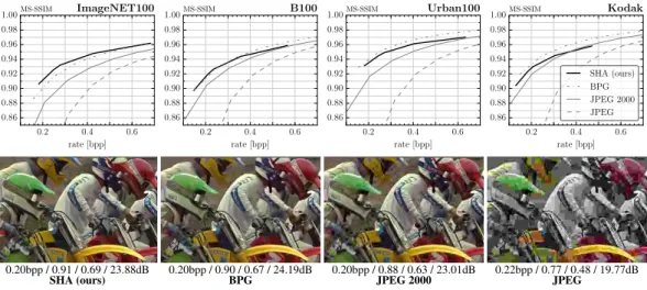
0.20bpp / 0.91 / 0.69 / 23.88dB 0.20bpp / 0.90 / 0.67 / 24.19dB 0.20bpp / 0.88 / 0.63 / 23.01dB 0.22bpp / 0.77 / 0.48 / 19.77dB
SHA (ours) BPG JPEG 2000 JPEG
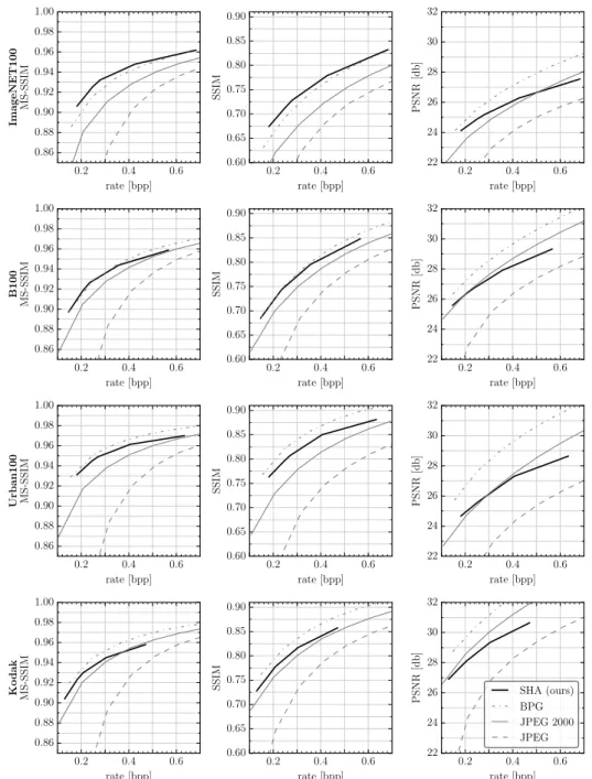
Figure 1: Top: MS-SSIM as a function of rate for SHA (Ours), BPG, JPEG 2000, JPEG, for each data set. Bottom: A visual example from the Kodak data set along with rate / MS-SSIM / SSIM / PSNR.
We trained different models using Adam [17], see Appendix A.2. Our training set is composed similarly to that described in [3]. We used a subset of 90,000 images from ImageNET [8], which we downsampled by a factor 0.7 and trained on crops of128×128pixels, with a batch size of 15.
To estimate the probability distributionpfor optimizing (8), we maintain a histogram over 5,000 images, which we update every 10 iterations with the images from the current batch. Details about other hyperparameters can be found in Appendix A.2.
The training of our autoencoder network takes place in two stages, where we move from an identity function in the bottleneck to hard quantization. In the first stage, we train the autoencoder without any quantization. Similar to [30] we gradually unfreeze the channels in the bottleneck during training (this gives a slight improvement over learning all channels jointly from the start). This yields an efficient weight initialization and enables us to then initializeσ0andCas described above. In the second stage, we minimize (6), jointly learning network weights and quantization levels. We annealσby letting the gap between soft and hard quantization error go to zero as the number of iterationstgoes to infinity.
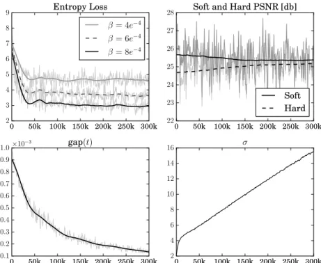
LeteS=kF(x)˜ −xk2be the soft error,eH=kFˆ(x)−xk2be the hard error. With gap(t) =eH−eS we can denote the error between the actual the desired gap witheG(t) =gap(t)−T /(T+t)gap(0), such that the gap is halved afterTiterations. We updateσaccording toσ(t+ 1) =σ(t) +KGeG(t), whereσ(t)denotesσat iterationt. Fig. 3 in Appendix A.4 shows the evolution of the gap, soft and hard loss as sigma grows during training. We observed that both vector quantization and entropy loss lead to higher compression rates at a given reconstruction MSE compared to scalar quantization and training without entropy loss, respectively (see Appendix A.3 for details).
Evaluation. To evaluate the image compression performance of our Soft-to-Hard Autoencoder (SHA) method we use four datasets, namely Kodak [1], B100 [31], Urban100 [14], ImageNET100 (100 randomly selected images from ImageNET [25]) and three standard quality measures, namely peak signal-to-noise ratio (PSNR), structural similarity index (SSIM) [37], and multi-scale SSIM (MS-SSIM), see Appendix A.5 for details. We compare our SHA with the standard JPEG, JPEG 2000, and BPG [10], focusing on compression rates<1bits per pixel (bpp) (i.e., the regime where traditional integral transform-based compression algorithms are most challenged). As shown in Fig. 1, for high compression rates (< 0.4bpp), our SHA outperforms JPEG and JPEG 2000 in terms of MS-SSIM and is competitive with BPG. A similar trend can be observed for SSIM (see Fig. 4 in Appendix A.6 for plots of SSIM and PSNR as a function of bpp). SHA performs best on ImageNET100 and is most challenged on Kodak when compared with JPEG 2000. Visually, SHA-compressed images have fewer artifacts than those compressed by JPEG 2000 (see Fig. 1, and Appendix A.7).
Related methods and discussion. JPEG 2000 [29] uses wavelet-based transformations and adap- tive EBCOT coding. BPG [10], based on a subset of the HEVC video compression standard, is the
ACC COMP.
METHOD [%] RATIO
ORIGINAL MODEL 92.6 1.00
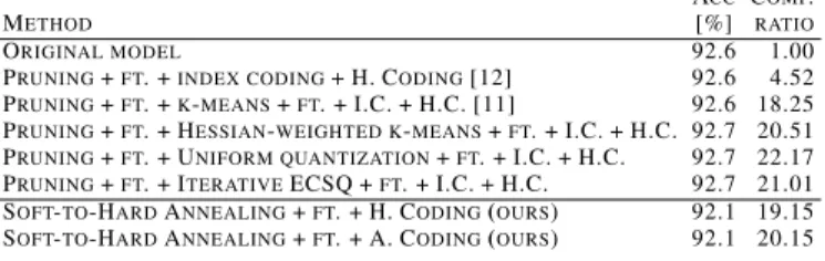
PRUNING+FT. +INDEX CODING+ H. CODING[12] 92.6 4.52 PRUNING+FT. +K-MEANS+FT. + I.C. + H.C. [11] 92.6 18.25 PRUNING+FT. + HESSIAN-WEIGHTED K-MEANS+FT. + I.C. + H.C. 92.7 20.51 PRUNING+FT. + UNIFORM QUANTIZATION+FT. + I.C. + H.C. 92.7 22.17 PRUNING+FT. + ITERATIVEECSQ +FT. + I.C. + H.C. 92.7 21.01 SOFT-TO-HARDANNEALING+FT. + H. CODING(OURS) 92.1 19.15 SOFT-TO-HARDANNEALING+FT. + A. CODING(OURS) 92.1 20.15
Table 1: Accuracies and compression factors for different DNN compression techniques, using a 32-layer ResNet on CIFAR-10. FT. denotes fine-tuning, IC. denotes index coding and H.C. and A.C.
denote Huffman and arithmetic coding, respectively. The pruning based results are from [5].
current state-of-the art for image compression. It uses context-adaptive binary arithmetic coding (CABAC) [21].
SHA (ours) Theiset al.[30]
Quantization vector quantization rounding to integers Backpropagation grad. of soft relaxation grad. of identity mapping Entropy estimation (soft) histogram Gaussian scale mixtures Training material ImageNET high quality Flickr images Operating points single model ensemble
The recent works of [30, 4]
also showed competitive perfor- mance with JPEG 2000. While we use the architecture of [30], there are stark differences be- tween the works, summarized
in the inset table. The work of [4] build a deep model using multiple generalized divisive normaliza- tion (GDN) layers and their inverses (IGDN), which are specialized layers designed to capture local joint statistics of natural images. Furthermore, they model marginals for entropy estimation using linear splines and also use CABAC[21] coding. Concurrent to our work, the method of [16] builds on the architecture proposed in [33], and shows that impressive performance in terms of the MS-SSIM metric can be obtained by incorporating it into the optimization (instead of just minimizing the MSE).
In contrast to the domain-specific techniques adopted by these state-of-the-art methods, our framework for learning compressible representation can realize a competitive image compression system, only using a convolutional autoencoder and simple entropy coding.
5 DNN Compression
For DNN compression, we investigate the ResNet [13] architecture for image classification. We adopt the same setting as [5] and consider a 32-layer architecture trained for CIFAR-10 [18]. As in [5], our goal is to learn a compressible representation for all 464,154 trainable parameters of the model.
We concatenate the parameters into a vectorW∈R464,154and employ scalar quantization (m=d), such thatZT =z=W. We started from the pre-trained original model, which obtains a92.6%
accuracy on the test set. We implemented the entropy minimization by usingL= 75centers and choseβ= 0.1such that the converged entropy would give a compression factor≈20,i.e., giving
≈32/20 = 1.6bits per weight. The training was performed with the same learning parameters as the original model was trained with (SGD with momentum0.9). The annealing schedule used was a simple exponential one,σ(t+ 1) = 1.001·σ(t)withσ(0) = 0.4. After 4 epochs of training, when σ(t)has increased by a factor≈20, we switched to hard assignments and continued fine-tuning at a10×lower learning rate.2Adhering to the benchmark of [5, 12, 11], we obtain the compression factor by dividing the bit cost of storing the uncompressed weights as floats (464,154×32bits) with the total encoding cost of compressed weights (i.e.,L×32bits for the centers plus the size of the compressed index stream).
Our compressible model achieves a comparable test accuracy of92.1%while compressing the DNN by a factor19.15with Huffman and20.15using arithmetic coding. Table 1 compares our results with state-of-the-art approaches reported by [5]. We note that while the top methods from the literature also achieve accuracies above92%and compression factors above20×, they employ a considerable amount of hand-designed steps, such as pruning, retraining, various types of weight clustering, special encoding of the sparse weight matrices into an index-difference based format and then finally use entropy coding. In contrast, we directly minimize the entropy of the weights in the training, obtaining a highly compressible representation using standard entropy coding.
2We switch to hard assignments since we can get large gradients for weights that are equally close to two centers asQ˜converges to hard nearest neighbor assignments. One could also employ simple gradient clipping.
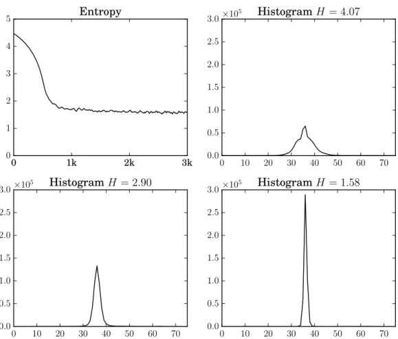
In Fig. 5 in Appendix A.8, we show how the sample entropyH(p)decays and the index histograms develop during training, as the network learns to condense most of the weights to a couple of centers when optimizing (6). In contrast, the methods of [12, 11, 5] manually impose0as the most frequent center by pruning≈80%of the network weights. We note that the recent works by [34] also manages to tackle the problem in a single training procedure, using the minimum description length principle.
In contrast to our framework, they take a Bayesian perspective and rely on a parametric assumption on the symbol distribution.
6 Conclusions
In this paper we proposed a unified framework for end-to-end learning of compressed representations for deep architectures. By training with a soft-to-hard annealing scheme, gradually transferring from a soft relaxation of the sample entropy and network discretization process to the actual non- differentiable quantization process, we manage to optimize the rate distortion trade-off between the original network loss and the entropy. Our framework can elegantly capture diverse compression tasks, obtaining results competitive with state-of-the-art for both image compression as well as DNN compression. The simplicity of our approach opens up various directions for future work, since our framework can be easily adapted for other tasks where a compressible representation is desired.
References
[1] Kodak PhotoCD dataset.http://r0k.us/graphics/kodak/, 1999.
[2] Eugene L Allgower and Kurt Georg. Numerical continuation methods: an introduction, volume 13. Springer Science & Business Media, 2012.
[3] Johannes Ballé, Valero Laparra, and Eero P Simoncelli. End-to-end optimization of nonlinear transform codes for perceptual quality. arXiv preprint arXiv:1607.05006, 2016.
[4] Johannes Ballé, Valero Laparra, and Eero P Simoncelli. End-to-end optimized image compres- sion.arXiv preprint arXiv:1611.01704, 2016.
[5] Yoojin Choi, Mostafa El-Khamy, and Jungwon Lee. Towards the limit of network quantization.
arXiv preprint arXiv:1612.01543, 2016.
[6] Matthieu Courbariaux, Yoshua Bengio, and Jean-Pierre David. Binaryconnect: Training deep neural networks with binary weights during propagations. InAdvances in Neural Information Processing Systems, pages 3123–3131, 2015.
[7] Thomas M Cover and Joy A Thomas. Elements of information theory. John Wiley & Sons, 2012.
[8] J. Deng, W. Dong, R. Socher, L.-J. Li, K. Li, and L. Fei-Fei. ImageNet: A Large-Scale Hierarchical Image Database. InCVPR09, 2009.
[9] Andre Esteva, Brett Kuprel, Roberto A Novoa, Justin Ko, Susan M Swetter, Helen M Blau, and Sebastian Thrun. Dermatologist-level classification of skin cancer with deep neural networks.
Nature, 542(7639):115–118, 2017.
[10] Bellard Fabrice. BPG Image format. https://bellard.org/bpg/, 2014.
[11] Song Han, Huizi Mao, and William J Dally. Deep compression: Compressing deep neural net- works with pruning, trained quantization and huffman coding.arXiv preprint arXiv:1510.00149, 2015.
[12] Song Han, Jeff Pool, John Tran, and William Dally. Learning both weights and connections for efficient neural network. InAdvances in Neural Information Processing Systems, pages 1135–1143, 2015.
[13] Kaiming He, Xiangyu Zhang, Shaoqing Ren, and Jian Sun. Deep residual learning for image recognition. InIEEE Conference on Computer Vision and Pattern Recognition (CVPR), June 2016.
[14] Jia-Bin Huang, Abhishek Singh, and Narendra Ahuja. Single image super-resolution from transformed self-exemplars. InProceedings of the IEEE Conference on Computer Vision and Pattern Recognition, pages 5197–5206, 2015.
[15] Itay Hubara, Matthieu Courbariaux, Daniel Soudry, Ran El-Yaniv, and Yoshua Bengio. Quan- tized neural networks: Training neural networks with low precision weights and activations.
arXiv preprint arXiv:1609.07061, 2016.
[16] Nick Johnston, Damien Vincent, David Minnen, Michele Covell, Saurabh Singh, Troy Chinen, Sung Jin Hwang, Joel Shor, and George Toderici. Improved lossy image compression with priming and spatially adaptive bit rates for recurrent networks.arXiv preprint arXiv:1703.10114, 2017.
[17] Diederik P. Kingma and Jimmy Ba. Adam: A method for stochastic optimization. CoRR, abs/1412.6980, 2014.
[18] Alex Krizhevsky and Geoffrey Hinton. Learning multiple layers of features from tiny images.
2009.
[19] Alex Krizhevsky and Geoffrey E Hinton. Using very deep autoencoders for content-based image retrieval. InESANN, 2011.
[20] Alex Krizhevsky, Ilya Sutskever, and Geoffrey E Hinton. Imagenet classification with deep convolutional neural networks. InAdvances in neural information processing systems, pages 1097–1105, 2012.
[21] Detlev Marpe, Heiko Schwarz, and Thomas Wiegand. Context-based adaptive binary arithmetic coding in the h. 264/avc video compression standard.IEEE Transactions on circuits and systems for video technology, 13(7):620–636, 2003.
[22] D. Martin, C. Fowlkes, D. Tal, and J. Malik. A database of human segmented natural images and its application to evaluating segmentation algorithms and measuring ecological statistics.
InProc. Int’l Conf. Computer Vision, volume 2, pages 416–423, July 2001.
[23] Mohammad Rastegari, Vicente Ordonez, Joseph Redmon, and Ali Farhadi. Xnor-net: Imagenet classification using binary convolutional neural networks. InEuropean Conference on Computer Vision, pages 525–542. Springer, 2016.
[24] Kenneth Rose, Eitan Gurewitz, and Geoffrey C Fox. Vector quantization by deterministic annealing. IEEE Transactions on Information theory, 38(4):1249–1257, 1992.
[25] Olga Russakovsky, Jia Deng, Hao Su, Jonathan Krause, Sanjeev Satheesh, Sean Ma, Zhiheng Huang, Andrej Karpathy, Aditya Khosla, Michael Bernstein, Alexander C. Berg, and Li Fei-Fei.
ImageNet Large Scale Visual Recognition Challenge. International Journal of Computer Vision (IJCV), 115(3):211–252, 2015.
[26] Wenzhe Shi, Jose Caballero, Ferenc Huszár, Johannes Totz, Andrew P Aitken, Rob Bishop, Daniel Rueckert, and Zehan Wang. Real-time single image and video super-resolution using an efficient sub-pixel convolutional neural network. InProceedings of the IEEE Conference on Computer Vision and Pattern Recognition, pages 1874–1883, 2016.
[27] Wenzhe Shi, Jose Caballero, Lucas Theis, Ferenc Huszar, Andrew Aitken, Christian Ledig, and Zehan Wang. Is the deconvolution layer the same as a convolutional layer? arXiv preprint arXiv:1609.07009, 2016.
[28] David Silver, Aja Huang, Chris J Maddison, Arthur Guez, Laurent Sifre, George Van Den Driess- che, Julian Schrittwieser, Ioannis Antonoglou, Veda Panneershelvam, Marc Lanctot, et al. Mas- tering the game of go with deep neural networks and tree search. Nature, 529(7587):484–489, 2016.
[29] David S. Taubman and Michael W. Marcellin.JPEG 2000: Image Compression Fundamentals, Standards and Practice. Kluwer Academic Publishers, Norwell, MA, USA, 2001.
[30] Lucas Theis, Wenzhe Shi, Andrew Cunningham, and Ferenc Huszar. Lossy image compression with compressive autoencoders. InICLR 2017, 2017.
[31] Radu Timofte, Vincent De Smet, and Luc Van Gool. A+: Adjusted Anchored Neighborhood Regression for Fast Super-Resolution, pages 111–126. Springer International Publishing, Cham, 2015.
[32] George Toderici, Sean M O’Malley, Sung Jin Hwang, Damien Vincent, David Minnen, Shumeet Baluja, Michele Covell, and Rahul Sukthankar. Variable rate image compression with recurrent neural networks. arXiv preprint arXiv:1511.06085, 2015.
[33] George Toderici, Damien Vincent, Nick Johnston, Sung Jin Hwang, David Minnen, Joel Shor, and Michele Covell. Full resolution image compression with recurrent neural networks. arXiv preprint arXiv:1608.05148, 2016.
[34] Karen Ullrich, Edward Meeds, and Max Welling. Soft weight-sharing for neural network compression. arXiv preprint arXiv:1702.04008, 2017.
[35] Gregory K Wallace. The JPEG still picture compression standard. IEEE transactions on consumer electronics, 38(1):xviii–xxxiv, 1992.
[36] Z. Wang, E. P. Simoncelli, and A. C. Bovik. Multiscale structural similarity for image quality assessment. InAsilomar Conference on Signals, Systems Computers, 2003, volume 2, pages 1398–1402 Vol.2, Nov 2003.
[37] Zhou Wang, A. C. Bovik, H. R. Sheikh, and E. P. Simoncelli. Image quality assessment: from error visibility to structural similarity.IEEE Transactions on Image Processing, 13(4):600–612, April 2004.
[38] Wei Wen, Chunpeng Wu, Yandan Wang, Yiran Chen, and Hai Li. Learning structured sparsity in deep neural networks. InAdvances in Neural Information Processing Systems, pages 2074–2082, 2016.
[39] Ronald J Williams. Simple statistical gradient-following algorithms for connectionist reinforce- ment learning. Machine learning, 8(3-4):229–256, 1992.
[40] Ian H. Witten, Radford M. Neal, and John G. Cleary. Arithmetic coding for data compression.
Commun. ACM, 30(6):520–540, June 1987.
[41] Paul Wohlhart, Martin Kostinger, Michael Donoser, Peter M. Roth, and Horst Bischof. Optimiz- ing 1-nearest prototype classifiers. InIEEE Conf. on Computer Vision and Pattern Recognition (CVPR), June 2013.
[42] Eyal Yair, Kenneth Zeger, and Allen Gersho. Competitive learning and soft competition for vector quantizer design.IEEE transactions on Signal Processing, 40(2):294–309, 1992.
[43] Aojun Zhou, Anbang Yao, Yiwen Guo, Lin Xu, and Yurong Chen. Incremental network quanti- zation: Towards lossless cnns with low-precision weights. arXiv preprint arXiv:1702.03044, 2017.
A Image Compression Details
A.1 Architecture
We rely on a variant of the compressive autoencoder proposed recently in [30], using convolutional neural networks for the image encoder and image decoder3. The first two convolutional layers in the image encoder each downsample the input image by a factor 2 and collectively increase the number of channels from 3 to 128. This is followed by three residual blocks, each with 128 filters. Another convolutional layer then downsamples again by a factor 2 and decreases the number of channels toc, wherecis a hyperparameter ([30] use 64 and 96 channels). For aw×h-dimensional input image, the output of the image encoder is thew/8×h/8×c-dimensional “bottleneck tensor”.
The image decoder then mirrors the image encoder, using upsampling instead of downsampling, and deconvolutions instead of convolutions, mapping the bottleneck tensor into aw×h-dimensional output image. In contrast to the “subpixel” layers [26, 27] used in [30], we use standard deconvolutions for simplicity.
A.2 Hyperparameters
We do vector quantization toL= 1000centers, using(pw, ph) = (2,2),i.e.,m=d/(2·2).We trained different combinations ofβandcto explore different rate-distortion tradeoffs (measuring distortion in MSE). Asβcontrols to which extent the network minimizes entropy,βdirectly controls bpp (see top left plot in Fig. 3). We evaluated all pairs(c, β)withc∈ {8,16,32,48}andmβ∈ {1e−4, . . . ,9e−4}, and selected 5 representative pairs (models) with average bpps roughly corresponding to uniformly spread points in the interval[0.1,0.8]bpp. This defines a “quality index” for our model family, analogous to the JPEG quality factor.
We experimented with the other training parameters on a setup withc = 32, which we chose as follows. In the first stage we train for250kiterations using a learning rate of1e−4. In the second stage, we use an annealing schedule withT = 50k, KG= 100, over800kiterations using a learning rate of1e−5. In both stages, we use a weakl2regularizer over all learnable parameters, withλ= 1e−12. A.3 Effect of Vector Quantization and Entropy Loss
0.2 0.4 0.6
rate [bpp]
22 24 26 28 30 32
PSNR[db]
Vector,β >0 Scalar,β >0 Vector,β= 0 JPEG
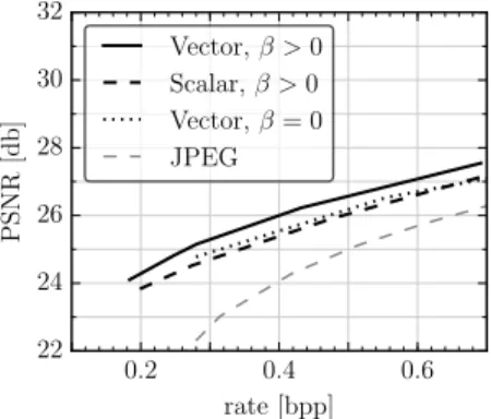
Figure 2: PSNR on ImageNET100 as a function of the rate for2×2-dimensional centers (Vector), for 1×1-dimensional centers (Scalar), and for2×2-dimensional centers without entropy loss (β = 0).
JPEG is included for reference.
To investigate the effect of vector quantization, we trained models as described in Section 4, but instead of using vector quantization, we setL= 6and quantized to1×1-dimensional (scalar) centers, i.e.,(ph, pw) = (1,1), m=d. Again, we chose 5 representative pairs(c, β). We choseL= 6to get approximately the same number of unique symbol assignments as for2×2patches,i.e.,64≈1000.
To investigate the effect of the entropy loss, we trained models using 2 ×2 centers for c ∈ {8,16,32,48}(as described above), but usedβ = 0.
Fig. 2 shows how both vector quantization and entropy loss lead to higher compression rates at a given reconstruction MSE compared to scalar quantization and training without entropy loss, respectively.
3We note that the image encoder (decoder) refers to the left (right) part of the autoencoder, which encodes (decodes) the data to (from) the bottleneck (not to be confused with the symbol encoder (decoder) in Section 3).
A.4 Effect of Annealing
0 50k 100k 150k 200k 250k 300k 2
3 4 5 6 7 8
9 Entropy Loss
β= 4e−4 β= 6e−4 β= 8e−4
0 50k 100k 150k 200k 250k 300k 22
23 24 25 26 27
28 Soft and Hard PSNR [db]
Soft Hard
0 50k 100k 150k 200k 250k 300k 0.1
0.2 0.3 0.4 0.5 0.6 0.7 0.8 0.9
1.0×10⁻³ gap(t)
0 50k 100k 150k 200k 250k 300k 2
4 6 8 10 12 14
16 σ
Figure 3: Entropy loss for threeβvalues, soft and hard PSNR, as well as gap(t)andσas a function of the iterationt.
A.5 Data Sets and Quality Measure Details
Kodak[1] is the most frequently employed dataset for analizing image compression performance in recent years. It contains 24 color768×512images covering a variety of subjects, locations and lighting conditions.
B100[31] is a set of 100 content diverse color481×321test images from the Berkeley Segmentation Dataset [22].
Urban100[14] has 100 color images selected from Flickr with labels such as urban, city, architecture, and structure. The images are larger than those from B100 or Kodak, in that the longer side of an image is always bigger than 992 pixels. Both B100 and Urban100 are commonly used to evaluate image super-resolution methods.
ImageNET100contains 100 images randomly selected by us from ImageNET [25], also downsam- pled and cropped, see above.
Quality measures. PSNR (peak signal-to-noise ratio) is a standard measure in direct monotonous relation with the mean square error (MSE) computed between two signals. SSIM and MS-SSIM are the structural similarity index [37] and its multi-scale SSIM computed variant [36] proposed to measure the similarity of two images. They correlate better with human perception than PSNR.
We compute quantitative similarity scores between each compressed image and the corresponding uncompressed image and average them over whole datasets of images. For comparison with JPEG we used libjpeg4, for JPEG 2000 we used the Kakadu implementation5, subtracting in both cases the size of the header from the file size to compute the compression rate. For comparison with BPG we used the reference implementation6and used the value reported in thepicture_data_length header field as file size.
4http://libjpeg.sourceforge.net/
5http://kakadusoftware.com/
6https://bellard.org/bpg/
A.6 Image Compression Performance
0.2 0.4 0.6
rate [bpp]
0.86 0.88 0.90 0.92 0.94 0.96 0.98 1.00
ImageNET100 MS-SSIM
0.2 0.4 0.6
rate [bpp]
0.60 0.65 0.70 0.75 0.80 0.85 0.90
SSIM
0.2 0.4 0.6
rate [bpp]
22 24 26 28 30 32
PSNR[db]
0.2 0.4 0.6
rate [bpp]
0.86 0.88 0.90 0.92 0.94 0.96 0.98 1.00
B100 MS-SSIM
0.2 0.4 0.6
rate [bpp]
0.60 0.65 0.70 0.75 0.80 0.85 0.90
SSIM
0.2 0.4 0.6
rate [bpp]
22 24 26 28 30 32
PSNR[db]
0.2 0.4 0.6
rate [bpp]
0.86 0.88 0.90 0.92 0.94 0.96 0.98 1.00
Urban100 MS-SSIM
0.2 0.4 0.6
rate [bpp]
0.60 0.65 0.70 0.75 0.80 0.85 0.90
SSIM
0.2 0.4 0.6
rate [bpp]
22 24 26 28 30 32
PSNR[db]
0.2 0.4 0.6
rate [bpp]
0.86 0.88 0.90 0.92 0.94 0.96 0.98 1.00
Kodak MS-SSIM
0.2 0.4 0.6
rate [bpp]
0.60 0.65 0.70 0.75 0.80 0.85 0.90
SSIM
0.2 0.4 0.6
rate [bpp]
22 24 26 28 30 32
PSNR[db]
SHA (ours) BPG JPEG 2000 JPEG
Figure 4: Average MS-SSIM, SSIM, and PSNR as a function of the rate for the ImageNET100, Urban100, B100 and Kodak datasets.
A.7 Image Compression Visual Examples
An online supplementary of visual examples is available athttp://www.vision.ee.ethz.ch/
~aeirikur/compression/visuals2.pdf, showing the output of compressing the first four images of each of the four datasets with our method, BPG, JPEG, and JPEG 2000, at low bitrates.
A.8 DNN Compression: Entropy and Histogram Evolution
0 1k 2k 3k
0 1 2 3 4
5 Entropy
0 10 20 30 40 50 60 70
0.0 0.5 1.0 1.5 2.0 2.5
3.0×10⁵ HistogramH = 4.07
0 10 20 30 40 50 60 70
0.0 0.5 1.0 1.5 2.0 2.5
3.0×10⁵ HistogramH = 2.90
0 10 20 30 40 50 60 70
0.0 0.5 1.0 1.5 2.0 2.5
3.0×10⁵ HistogramH = 1.58
Figure 5: We show how the sample entropyH(p)decays during training, due to the entropy loss term in (6), and corresponding index histograms at three time instants. Top left: Evolution of the sample entropyH(p). Top right: the histogram for the entropyH = 4.07att= 216. Bottom left and right: the corresponding sample histogram whenH(p)reaches2.90bits per weight att= 475 and the final histogram forH(p) = 1.58bits per weight att= 520.