Blackwell Publishing Ltd
Co-existence of divergent communities at natural boundaries: spider (Arachnida: Araneae) diversity across an alpine timberline
PAT R I C K M U F F ,
1C H R I S T I A N K R O P F ,
1H O L G E R F R I C K ,
1W O L F G A N G N E N T W I G
2a n d M A R T I N H . S C H M I D T- E N T L I N G
2 1Department of Invertebrates, Natural History Museum Bern, Bernastrasse 15, Bern, Switzerland, and
2Zoological Institute, University of Bern, Baltzerstrasse 6, Bern, Switzerland
Abstract. 1. Habitat boundaries can contain high biodiversity because they potentially combine species from two habitat types plus additional boundary specialists. However, most research on animal communities is focused on uniform habitats.
2. Here, we assessed the degree to which the community change at a habitat edge is determined by the broad-scale spatial transition from one habitat to the other, or by fine- scale environmental influences. We compared the distribution of ground-dwelling spider species from open land to forest with the distribution around stand-alone trees at the boundary, the alpine timberline (Grisons, Switzerland).
3. Our results showed that spiders were more strongly influenced by local environ- mental conditions (40% of explained variation) than by the spatial position within the ecotone (24.5% of explained variation, with 15.6% overlap between the two). Spider communities differentiated according to light availability and corresponding changes in the ground vegetation.
4. Since the small area around a single tree at the studied timberline offered a similar broad spectrum of environmental conditions as the open land and forest together, it pro- vided both habitats for species from the adjoining open land and forest as well as for some possible timberline specialists.
5. Accordingly, natural habitat boundaries may maintain very contrasting communities by providing a wide range of habitat conditions.
Key words. Arthropods, dwarf-shrub heath, ecotone, environment and space, forest, light, microspatial distribution, pitfall traps, Swiss Central Alps, vegetation structure.
Introduction
Spatial patterning of landscapes and its influence on the abundance and distribution of organisms remains one of the most fundamental issues in ecology (Ricklefs, 2004; Rahbek, 2005).
Ecosystem management requires an understanding of the factors that drive species diversity. Landscapes exist as mosaics of numerous different patch types that interact with each other.
Hence, knowledge about the ecology of habitat edges is critical for understanding which resources and interactions determine the distribution of organisms (Ries et al., 2004). As land-use
pressure often reduces the area of boundary habitats, their value in the conservation of habitats and species should be investigated (Harrison & Bruna, 1999; Brooks, 2000; Channell & Lomolino, 2000). Edges can be defined as ecotones between two plant communities, which are the transition zones between these communities (Holland et al., 1991). The specific characteristics and value of the ecotonal flora and fauna have been known for a long time as ‘edge effects’, which are manifested as high diversity in microhabitats, a change in abiotic factors and species interactions and elevated species richness (Odum, 1971;
Matlack, 1993; Murcia, 1995; Laurance et al., 2002). Recently, ecotones were even found to be sources of speciation (Smith et al., 1997; Schilthuizen, 2000).
However, our knowledge about biotic patterns and processes across natural boundaries and their extrapolation to landscapes
Correspondence: P. Muff, Department of Invertebrates, NaturalHistory Museum Bern, Bernastrasse 15, CH-3005 Bern, Switzerland.
E-mail: patrick.muff@gmail.com
is still limited (Ries et al., 2004). Only a small proportion of the edge literature deals with arthropods, although they account for the largest part of animal biodiversity (Wilson, 1992). Arthropods are important in a range of ecological processes (Didham et al., 1996), which should make them a main target for conservation.
Existing studies on arthropods at habitat boundaries are often focused on anthropogenically created edges around clear-cuts, plantations or arable land (Duelli et al., 1990; Downie et al., 1996; Martin & Major, 2001; Rand et al., 2006; Matveinen-Huju et al., 2006). Comparatively few investigations have addressed natural ecosystems within the scope of edge ecology and arthro- pods (but see Heublein, 1983; Hänggi & Baur, 1998; Kotze &
Samways, 2001; Magura et al., 2001; Ferguson, 2004). Still, these systems may provide advantages in assessing habitat asso- ciations and spatial patterns of organisms due to their equilib- rium conditions and more stable populations (Maurer, 1980;
Ricklefs, 2004).
In this empirical study, we investigated the differentiation of epigeic spider communities across a natural boundary, the alpine timberline. We chose spiders as study organisms because they are abundant, species rich, and known to have well-defined habitat preferences (Cherrett, 1964; Coddington & Levi, 1991;
Wise, 1993; Foelix, 1996), which makes them sensitive to edge effects and suitable for studying organism–habitat relationships.
Moreover, because they are at the top of invertebrate food chains (Wise, 1993), spiders are likely to play an important role in shaping terrestrial arthropod communities and may therefore influence the distributions of other arthropods. The importance of vegetation structure in influencing spider distribution has long been noted (Robinson, 1981; Uetz, 1991; Downie et al., 1995).
Recently, Frick et al. (2007) were able to show that a single spruce tree at the timberline offers habitats for a wide range of spider species with different abiotic requirements. It has been assumed that these requirements can be described as environ- mental gradients in moisture and shading, respectively (Huhta, 1971; Wise, 1993; Ferguson, 2004), which was confirmed in a recent analysis across Central Europe (Entling et al., 2007).
However, we still do not know the unique and quantitative contribution of moisture and shading and the relative influence of other variables such as vegetation structure in determining spider distribution. Additionally, studies that differentiate between spatial and ecological influence are still scarce, although the importance of space in structuring communities has been discussed for years and approaches to integrate the new concepts into sta- tistical analysis are manifold. In the current study, we analysed to which degree the community change at the alpine timberline is determined by the broad-scale spatial transition from one habitat to the other, or by fine-scale environmental influences.
Moisture was relatively uniform across our study area due to the consistent inclination and the western exposition. We therefore focused on vegetation structure and the environmental gradient in shading. By investigating the spider distribution and its under- lying factors, we also aimed to assess the value of boundaries, for example, the alpine timberline, in maintaining invertebrate communities. We specifically addressed four questions: (i) is community change at a timberline characterised by a broad-scale spatial transition from the open land to forest, or by fine-scale environmental influences? (ii) is vegetation structure or light
more important in structuring epigeic spider communities? (iii) is an alpine timberline more species rich than the open land and forest, respectively? (iv) are there boundary species at a timberline that are absent from the adjoining habitats?
Methods
Study site
The study was conducted at Alp Flix (9°38′E, 46°31′N) in the Swiss Central Alps near the village of Sur in the canton Grisons, Switzerland. The alp is a southwest exposed terrace of 15 km
2at 1950 m above sea level. It is surrounded by 3000 m mountain peaks and a valley. Our study area was a 300-m long stretch of timberline plus fragments of the adjoining Norway spruce forest (Vaccinio-Piceion) to the west and of the dwarf-shrub heath (Juniperion nanae) to the east. Each of the three parts covered approximately 3 ha. The site is located on a small slope inclined slightly towards the forest and is used for occasional cattle grazing throughout the vegetation period.
Study design and spider sampling
We differentiated between five habitat zones: the open land (dwarf-shrub heath) and forest, representing two macrohabitats, and three microhabitats linked to a single spruce tree at the timberline. These three microhabitats were defined by their location relative to the tree as: (i) next to the trunk (in figures and tables denoted as timberline trunk), (ii) at the end of branch cover (timberline branch), and (iii) in the adjoining open area outside of branch cover (timberline open). These five zones represented the whole gradient of habitat structures from forest to open land and thus allowed us to compare the macrospatial gradient across these two habitats with the microspatial gradient across the three areas around a tree.
In each of the five different habitat zones, we placed 15 pitfall
traps. In the open land, forest and the open area at the timberline
the traps were randomly positioned at least 15 m apart from each
other. For placing the traps in the timberline zones at the end of
branch cover and next to the trunk, the tree nearest to the trap in
the open area at the timberline was chosen. Thus, the three
microhabitats at the timberline were sampled at each of fifteen
stand-alone trees. The mean distances between the traps in these
three microhabitats were 4.1 m (timberline open–timberline
branch), 4.5 m (timberline open–timberline trunk) and 1.5 m
(timberline branch–timberline trunk). The traps consisted of
white plastic cups with an upper diameter of 6.9 cm and a depth
of 7.5 cm filled with a solution of 4% formaldehyde in water
plus detergent (0.05% sodium dodecyl sulphate). Each trap was
covered with a quadrangular transparent plastic roof (15
×15 cm)
fixed by three wooden rods 8 cm above-ground. Due to the
proximity of cattle and the toxicity of the trapping liquid, we
fenced off each trap with three plastic poles connected with
ribbons. The traps were operated for 1 year. They were emptied
monthly during the snow-free period (May 2005 to October
2005) and then left under the snow layer until May 2006, when
they were emptied a last time. Only adult spiders were identified to species level, juveniles were excluded from the analyses.
Nomenclature followed Platnick (2007).
Environmental variables
Sixteen environmental variables were measured at each of the 75 trap sites (Table 1). Ten variables represent structural categories of vegetation cover and were estimated for a rectangular area of 9 m
2around each trap in June 2006. Tree branches were distinguished into close to ground (if below 50 cm) and distant from ground (if above 50 cm). Tree density (including trees higher than 2.5 m) and the number of trees below 2.5 m were calculated by counting the number of trees within a radius of 5 m. The proportion of visible sky and related available radiation (i.e. the fraction of direct radiation under the canopy relative to the direct radiation above the canopy) were obtained with hemispheric photographs taken with a Nikon Coolpix 900 digital camera with an FC-E9 fisheye lens attached on the SLM5 Hemiview Self Levelling Mount UM (Delta-T Devices Ltd, Burwell, Cambridge, UK) in July 2006 and the program hemiview 2.1.
Spatial variables
Techniques to integrate space into analyses of species distribution have greatly increased since Legendre and Fortin (1989). We used the geographical coordinates of all trap locations for assessing linear spatial gradients (Borcard &
Legendre, 2002). To allow a more detailed identification of the spatial patterns, we obtained 41 additional spatial variables in a principal coordinates of neighbour matrices (PCNM) analysis (Borcard & Legendre, 2002; Borcard et al., 2004) using the program
spacemaker 2 (Borcard & Legendre, 2003). PCNMvariables were obtained by principal coordinate analysis (PCoA) of a truncated matrix of distances among sites. As the largest
distance between two adjacent trap sites, we used a truncation distance of 75 m (Borcard & Legendre, 2002). This technique allowed to distinguish between spatial and environmental influences on spider distribution. Nevertheless, it must be noted that only the microhabitats within the timberline were spatially replicated in our study. As the macrohabitats were not replicated, the designation of species as typical for one of the macrohabitats is only valid for the study area, and must not be generalised. In the following, we use terms such as ‘forest spiders’ in the sense of forest spiders in our study area.
Statistical analysis
Numbers of spider individuals were pooled for each trap over the whole sampling period. Since the length of gradients was only 3.95 and 1.84 for the first two axes of a preliminary detrended correspondence analysis on spider communities (DCA), we used linear methods of ordination (ter Braak & Smilauer, 2002b). We conducted principal component analysis (PCA) to visualise the main trends of community variation across the habitat zones. The environmental variables recorded and the five habitat zones were included passively into the analysis for a first estimation of their influence (Fig. 1). Both analyses were run in the program canoco 4.5 for Windows (ter Braak & Smilauer, 2002a) on Hellinger-transformed species data (Legendre &
Gallagher, 2001). To measure the relative contribution of spatial and environmental variables in explaining the variation of species assemblages, we partitioned the explained variation (Borcard et al., 1992; Borcard & Legendre, 1994). This was achieved through a series of partial canonical redundancy analyses (RDA). We calculated the ‘marginal’ and ‘conditional’
effects of sets of environmental or spatial variables with the program
varcan 1.0 (Peres-Neto, 2006) adopting the testingprocedures described by Legendre and Legendre (1998).
Marginal effects denoted the variation explained by a given set without considering other variables, whereas conditional
Table 1. Environmental conditions (mean ± SE) in the five different habitat zones (for definitions see text). N= 15 for each habitat.Open land Timberline open Timberline branch Timberline trunk Forest
Open ground (percentage) 11 ± 2 9 ± 2 22 ± 3 31 ± 5 57 ± 7
Stone (percentage) 4 ± 1 3 ± 1 3 ± 0 3 ± 1 3 ± 1
Moss (percentage) 1 ± 0 3 ± 1 9 ± 2 9 ± 3 19 ± 4
Herb (percentage) 40 ± 5 36 ± 4 32 ± 3 25 ± 3 18 ± 6
Low dwarf-shrub (percentage) 26 ± 4 23 ± 4 20 ± 3 18 ± 3 2 ± 1
High dwarf-shrub (percentage) 20 ± 5 27 ± 5 18 ± 4 16 ± 3 2 ± 1
Branch close to ground (percentage) 0 ± 0 0 ± 0 20 ± 3 30 ± 4 2 ± 1
Branch distant from ground (percentage) 0 ± 0 2 ± 1 44 ± 4 68 ± 4 60 ± 8
Trunk (percentage) 0 ± 0 0 ± 0 1 ± 0 3 ± 1 3 ± 1
Small spruce (percentage) 1 ± 1 3 ± 1 4 ± 2 1 ± 1 0 ± 0
Tree smaller 2.5 m (nha–1) 8 ± 8 263 ± 72 246 ± 66 289 ± 82 246 ± 56
Tree density (nha–1) 0 ± 0 272 ± 49 373 ± 60 365 ± 63 1053 ± 107
Distance to closest trunk (metres) 41.6 ± 3.8 4.6 ± 0.6 1.4 ± 0.1 0.4 ± 0.1 1.8 ± 0.3
Distance to closest branch (metres) 40.1 ± 3.8 2.8 ± 0.4 0 ± 0 –1 ± 0.1 1.2 ± 0.3
Visible sky (percentage) 79 ± 1 63 ± 2 27 ± 2 14 ± 1 15 ± 0
Available radiation (percentage) 0.96 ± 0 0.79 ± 0.03 0.27 ± 0.04 0.10 ± 0.02 0.18 ± 0.02
effects denoted the variation explained by a given set after removing the confounding effect of one or more other variables.
varcan 1.0 also corrected for the biases in the method of
variation partitioning influenced by both the number of explanatory variables and sample size (Dray et al., 2006;
Peres-Neto et al., 2006). As explanatory variables, we used all 16 environmental variables recorded, since using the full set of predictors yields more accurate estimations of fractions than applying forward selection (Peres-Neto et al., 2006), as well as the geographical coordinates of all trap locations and the 41 PCNM variables (Fig. 2). The difference between two fractions of variation was tested by using 10 000 bootstrap samples. For estimating the marginal and conditional effects of each environmental variable on species variation, we contrasted them individually with the residual set of environmental predictors (Table 2).
To identify the compositional differences (= beta diversity) within and between assemblages of the five habitat zones (Table 3), we used permutational multivariate analysis of variance (Anderson,
Fig. 1. Principal component analysis (PCA) of spider communities at the 75 trap locations in the five different habitat zones. In (a) passively included environmental variables are represented by arrows; their relative effect on the community differentiation is indicated by the length and direction of the arrows. Only environmental variables accounting for major influences are shown. In (b) the mean positions of the five habitat zones are shown; numbers denote single species with N≥15 individuals (for names see Table 4).
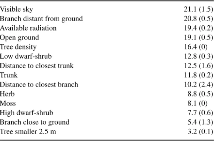
Table 2. Independent, marginal (and dependent, conditional) contribution (percentage) of selected single environmental variables in explaining the spider community structure.
Visible sky 21.1 (1.5)
Branch distant from ground 20.8 (0.5)
Available radiation 19.4 (0.2)
Open ground 19.1 (0.5)
Tree density 16.4 (0)
Low dwarf-shrub 12.8 (0.3)
Distance to closest trunk 12.5 (1.6)
Trunk 11.8 (0.2)
Distance to closest branch 10.2 (2.4)
Herb 8.8 (0.5)
Moss 8.1 (0)
High dwarf-shrub 7.7 (0.6)
Branch close to ground 5.4 (1.3)
Tree smaller 2.5 m 3.2 (0.1)
2001; McArdle & Anderson, 2001) on the basis of Bray–Curtis distance measure as implemented in the program
permanova(Anderson, 2005). For comparisons of abundance at the species level (Table 4), we used pairwise Kruskal–Wallis tests (k = 9999 Monte Carlo permutations), because a Levene’s test indicated
that variances of the species data were not homogeneous.
These analyses were conducted with the program spss 14.0 for Windows including only species N
≥15 individuals. All P- values were corrected for multiple comparisons after Holm (Legendre & Legendre, 1998).
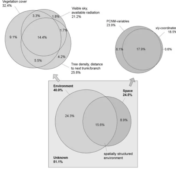
Fig. 2. Variation partitioning (percentage) of the pooled species data into different environmental and spatial components. The area of the square and circles are proportional to the fraction of total variation explained. Values outside the symbols: marginal effects; values inside the symbols: conditional effects (see text). The two fractions ‘environment’ and ‘space’ were significantly different (P= 0.02), whereas the influence of the x/y coordinate did not differ from the one of the PCNM-variables (P= 0.28). The component ‘vegetation cover’ includes all environmental variables not listed explicitly in this figure, apart from ‘tree smaller 2.5 m’, which is part of the component ‘tree density . . .’.
Table 3. Average Bray–Curtis dissimilarities within/between communities of all five habitat zones. Values in parentheses represent t-statistics of pairwise comparisons (all P< 0.001, corrected for multiple comparisons after Holm).
Open land Timberline open Timberline branch Timberline trunk Forest
Open land 48.5
Timberline open 54.5 (2.0) 49.9
Timberline branch 65.0 (3.3) 56.3 (2.1) 51.8
Timberline trunk 78.4 (4.3) 72.5 (3.6) 62.3 (2.4) 56.1
Forest 89.8 (5.4) 82.3 (4.6) 73.1 (3.6) 64.3 (2.4) 55.2
Results
Spider community differentiation
We captured 6251 adult spiders belonging to 102 species and 14 families. The spider communities of the five distinct habitat zones differed clearly in their species compositions (Fig. 1a).
The first PCA axis represented 30% of species variation. It correlated mainly with tree density and the proportion of visible sky and branch distant from ground, and separated the open land from forest. In representing another 11% of variation, the second axis separated the open land from the open area at the timberline, and (less clearly) the three different microhabitats within the timberline.
Variation partitioning revealed that 40% of variation in the species assemblages has been explained by the environment (Fig. 2). However, a large proportion of this variation (15.6% of the total variation explained) overlapped with the spatial structure of the environment. Together with a minor influence of pure spatial attributes (8.9%), almost 49% of species variation has been explained with the variables recorded. The influence of space resulted mainly from a linear gradient, represented by the x and y geographical coordinates, which alone determined 18.5%
of species distribution. The variation explained by the environ- ment was mainly attributable to factors directly influencing or resulting from the fraction of light reaching the ground (tree density, available radiation, proportion of visible sky, branch distant from ground and open ground). Most of them contributed about 20% of explanation each, although their influences over- lapped highly (Table 2). In contrast, the type of ground vegetation (proportion of dwarf-shrub heath, herb, moss and branch close to ground) did not contribute much to the differentiation of the communities.
The multivariate analysis of variance on the species data showed that the communities found in the five habitat zones dif- fered highly significantly from each other (F = 12.5, P = 0.0001).
The largest dissimilarity was found between the open land and forest (Table 3). The timberline zone next to the trunk differed most strongly from the open land, whereas the open area at the timberline differed most strongly from the forest. In contrast, the most similar assemblages have been found in the open area at the timberline and the open land, and in the timberline zone next to the trunk and the forest, respectively. Species composition in the timberline zone at the end of branch cover seemed to be most similar with the communities in the other two zones at the timberline. Interestingly, the difference within the five habitat zones increased gradually along the gradient from the open land to the forest (Table 3).
Habitat preferences
All five habitat zones were dominated by certain species (Fig. 1b, Table 4). Two species dominated significantly in the open land, two in the open area at the timberline and four in the forest. Three additional species were significantly more frequent in one of the zones at the timberline than in either forest or open land. A comparison of frequencies by percentage indicates that
most species seemed to prefer the open land whereas the forest was inhabited by a higher proportion of specialists. Regarding the zones at the timberline, the open area may have been most attractive followed by the zone next to the trunk. In contrast, few if any species seemed to prefer the zone at the end of branch cover.
Discussion
The distribution of epigeic spiders across the alpine timberline correlated most with the environmental factor light. Shading by woody plants is also the main factor for spider distribution among Central European lowland habitats (Entling et al., 2007). By offering both open and completely shaded microhabitats (Table 1), the small area around a single tree provided habitats for the majority of species present in both open land and forest (Table 4). As a result, the distribution of the species found in this study across an area of 9 ha corresponded fairly well to the distribution within a few metres (Fig. 1a). Our findings indicate that due to the sensitivity of spiders to their environment, the differentiation of communities can act also on a very small scale if the landscape is heterogeneous enough. The question remains, however, how viable populations are in habitats as small as the area around a single tree.
Factors driving spider community differentiation
Neutral theory of biodiversity and biogeography is able to reproduce certain patterns of species distribution without considering habitat conditions and niche properties (Hubbell, 2005). Nevertheless, the two classic models of communities shaped by environmental factors and biological interactions are still widely supported (Peterson & Holt, 2003; Eyre et al., 2005). The relationship between species diversity and habitat features seems to be strongly dependent on the organisms and region (Jeanneret et al., 2003;
Schweiger et al., 2005). Habitat preferences of spiders are well documented and several underlying environmental factors have been proposed (Samu et al., 1999; Entling et al., 2007). All of these factors deal with physical properties of the environment, which influence either light and moisture conditions or specific demands of spiders on their environment (e.g. places for hunting, courtship, prey availability, protection from enemies and desiccation). Because of interactions between environmental conditions and vegetation characteristics, the quantitative importance of these different factors has remained speculative. In our study, variables connected with light availability (e.g.
proportion of open ground and visible sky) had a greater influence on spider communities than the type of ground vegetation in which the spiders live (Fig. 1, Table 2). The rather large effect of the component ‘vegetation cover’ on species variation (Fig. 2) is a direct result of the inclusion of the two variables ‘open ground’
and ‘branches distant from ground’ into this component.
Our study demonstrates the possible overestimation of
environmental effects on species distribution when space is not
taken into account (Borcard et al., 1992). Space overlapped with
almost 40% of the total environmental influence and accounted
for 18% of the total variation explained (Fig. 2). This
demonstrates very impressively how ecological phenomena can be spatially structured and that species and physical variables are distributed neither uniformly nor at random (Legendre, 1993).
Pure spatial variation may reflect biological processes without relationship to the environmental variables recorded, such as growth, predation, competition, reproduction or social aggregation for example (Borcard et al., 1992). The high amount of unexplained variation can be understood by considering that it
may not only represent real stochasticity but also unmeasured, potentially explainable environmental effects.
Microspatial distribution at boundaries
Our study at the timberline indicates that also spatially limited structures can be of great importance in providing a wide range
Table 4. Numbers of spider individuals (N) and their distribution by percentage across the five habitat zones. The order follows the species’ dominance in one of the habitat zones (in bold). Letters behind numbers denote habitats significantly different from each other according to pairwise Kruskal–Wallis tests (all P< 0.05, corrected for multiple comparisons after Holm). Only species with N≥15 are shown. Codes refer to Fig. 1b. Mean number of individuals and species per pitfall trap, respectively, and Simpson diversity for each habitat zone are additionally included at the bottom.Code Species Family Total N Open land Timberline open Timberline branch Timberline trunk Forest
1 Meioneta alpica Linyphiidae 18 89b 11a 0a 0a 0a
2 Gnaphosa leporina Gnaphosidae 32 88b 9a 3a 0a 0a
3 Pardosa mixta Lycosidae 18 72b 22ab 6ab 0a 0a
4 Macrargus carpenteri Linyphiidae 42 69c 17bc 7abc 7ab 0a
5 Drassodes cupreus Gnaphosidae 20 60c 30bc 5ab 5ab 0a
6 Alopecosa pulverulenta Lycosidae 639 57c 37c 5b 0a 0a
7 Thanatus formicinus Philodromidae 59 56b 36b 8a 0a 0a
8 Alopecosa accentuata Lycosidae 26 54c 35bc 8abc 0a 4ab
9 Ozyptila atomaria Thomisidae 18 50c 28bc 17abc 6ab 0a
10 Zelotes talpinus Gnaphosidae 47 47b 38b 13ab 0a 2a
11 Pardosa blanda Lycosidae 150 44c 42bc 13ab 1ab 0a
12 Drassodes pubescens Gnaphosidae 27 41c 30bc 19abc 4a 7ab
13 Halpodrassus signifer Gnaphosidae 79 33c 32bc 15ab 10a 10a
14 Minicia marginella Linyphiidae 16 13a 69a 13a 6a 0a
15 Gonatium rubens Linyphiidae 22 18ab 59b 18ab 5a 0a
16 Arctosa renidescens Lycosidae 64 23ab 58b 13ab 5ab 2a
17 Bolyphantes luteolus Linyphiidae 109 23c 56d 12b 9b 0a
18 Agyneta cauta Linyphiidae 128 24c 55c 19bc 2ab 0a
19 Alopecosa taeniata Lycosidae 429 2a 52b 30b 7a 9a
20 Tenuiphantes mengei Linyphiidae 180 21b 44c 14b 16b 5a
21 Bolyphantes alticeps Linyphiidae 44 7ab 39b 23ab 2a 30ab
22 Xysticus luctuosus Thomisidae 40 15ab 38b 48b 0a 0a
23 Micaria aenea Gnaphosidae 48 15b 25b 44b 0a 17b
24 Metopobactrus prominulus Linyphiidae 15 13a 20a 40a 27a 0a
25 Caracladus avicula Linyphiidae 196 20ab 11a 38b 13ab 17ab
26 Pelecopsis radicicola Linyphiidae 84 10a 19ab 35b 30ab 7a
27 Pardosa riparia Lycosidae 1953 30c 27c 31c 11b 1a
28 Panamomops tauricornis Linyphiidae 70 0a 0a 3a 80b 17b
29 Scotinotylus alpigena Linyphiidae 146 0a 0a 5a 62b 33b
30 Pelecopsis elongata Linyphiidae 54 0a 0a 33b 50b 17ab
31 Mansuphantes pseudoarciger Linyphiidae 18 6a 22ab 11ab 50b 11ab
32 Improphantes nitidus Linyphiidae 136 1a 0a 3a 49b 46b
33 Scotargus pilosus Linyphiidae 17 0a 0a 18ab 47b 35ab
34 Tapinocyba affinis Linyphiidae 249 1a 8b 32c 44c 15b
35 Robertus truncorum Theridiidae 105 0a 9ab 31b 36b 24b
36 Mughiphantes cornutus Linyphiidae 23 0a 0a 9a 9a 83a
37 Cryphoeca silvicola Hahniidae 134 0a 0a 1a 25b 74c
38 Porrhomma pallidum Linyphiidae 42 0a 0a 7ab 19b 74c
39 Mughiphantes mughi Linyphiidae 38 0a 3ab 8ab 21b 68c
40 Agnyphantes expunctus Linyphiidae 52 0a 0a 12ab 31b 58c
41 Scotinotylus clavatus Linyphiidae 114 0a 0a 6ab 43bc 51c
42 Centromerus pabulator Linyphiidae 319 3a 30bc 25abc 10ab 32c
Mean number of individuals 100 112 89 65 51
Mean number of species 18 18 16 16 14
Simpson diversity 0.74 0.79 0.76 0.83 0.86
of habitats. These findings are consistent with other studies suggesting small-scale distribution of invertebrates. Antvogel and Bonn (2001) identified different ground beetle assemblages within a few metres in an alluvial forest; Maudsley et al. (2002) revealed highly spatially variable distribution patterns of overwintering arthropods within an individual hedgerow; Juen and Traugott (2004) found distinct spatial distribution patterns of arthropod predator communities in an organically cultivated 0.3-ha field and Romero and Vasconcellos-Neto (2005) demonstrated how changes in the architecture of a single plant species influences the microspatial distribution of a strictly associated spider species.
Furthermore, the current study underlines the suitability of boundary habitats for assessing distribution patterns and their determining factors, at least for invertebrates, which is essential for nature conservation. Due to the edge effects and their well-known influences on these organisms in patchy habitats (Downie et al., 1996; Magura et al., 2001) relationships can be investigated to a great extent, even when time and effort are restricted (Antvogel
& Bonn, 2001). Understanding the small-scale distribution of organisms reveals their suitability as bio-indicators, which today becomes increasingly important in the context of nature conservation and management (Spellerberg, 1993). The community differentiation between microhabitats around a single tree found in our study clearly confirms the suitability of spiders to indicate changes in habitats and the environment as suggested in other studies (Marc et al., 1999; Pearce & Vernier, 2006).
Conclusion
This study demonstrates how habitat boundaries may maintain very contrasting communities by providing a wide range of habitat conditions. The epigeic spider communities at an alpine timberline were strongly influenced by the local environment and differentiated according to light preferences of single species. The occurrence of nearly all species from the adjoining open land and forest patches as well as some possible habitat specialists around single trees at the timberline highlights the potential of heterogeneous microspatial structures in preserving arthropod communities.
Acknowledgements
We kindly thank Victoria Spinas for her continual enthusiastic support on the alp and the Foundation ‘Schatzinsel Alp Flix’, particularly Jürg Paul Müller, for offering free accommodation.
Eduard Jutzi and Lukas Zimmermann helped with technical equipment and Heather Murray provided valuable linguistic comments on the manuscript. For statistical advice, we thank Daniel Borcard, Anik Brind’Amour, Robert Colwell, Pierre Legendre, Pedro Peres-Neto, Thiago F. Rangel and Cajo ter Braak. This manuscript benefited substantially from comments by Tatyana Rand, Mary E.A. Whitehouse and two anonymous reviewers.
References
Anderson, M.J. (2001) A new method for non-parametric multivariate analysis of variance. Austral Ecology, 26, 32–46.
Anderson, M.J. (2005) PERMANOVA: A FORTRAN Computer Program for Permutational Multivariate Analysis of Variance. Department of Statistics, University of Auckland, New Zealand.
Antvogel, H. & Bonn, A. (2001) Environmental parameters and micro- spatial distribution of insects: a case study of carabids in an alluvial forest. Ecography 24, 470–482.
Borcard, D. & Legendre, P. (1994) Environmental control and spatial structure in ecological communities: an example using Oribatid mites (Acari, Oribatei). Environmental and Ecological Statistics, 1, 37–61.
Borcard, D. & Legendre, P. (2002) All-scale spatial analysis of ecological data by means of principal coordinates of neighbour matrices. Ecological Modelling, 153, 51–68.
Borcard, D. & Legendre, P. (2003) SPACEMAKER: Generates Spatial Explanatory Variables to Be Used in Multiple Regression or Canonical Ordination, Version 2. Available from URL: http://www.bio.umon- treal.ca/casgrain/en/labo/spacemaker.html.
Borcard, D., Legendre, P. & Drapeau, P. (1992) Partialling out the spatial component of ecological variation. Ecology, 73, 1045–1055.
Borcard, D., Legendre, P., Avois-Jacquet, C. & Tuomisto, H, (2004) Dissecting the spatial structure of ecological data at multiple scales.
Ecology, 85, 1826–1832.
Brooks, T. (2000) Living on the edge. Nature, 403, 26–28.
Channell, R. & Lomolino, M.V. (2000) Dynamic biogeography and con- servation of endangered species. Nature, 403, 84–86.
Cherrett, J.M. (1964) The distribution of spiders on the Moor House Nature Reserve, Westmorland. Journal of Animal Ecology, 33, 27–48.
Coddington, J.A. & Levi, H.W. (1991) Systematics and evolution of spiders (Araneae). Annual Review of Ecology and Systematics, 22, 565–592.
Didham, R.K., Ghazoul, J., Stork, N.E. & Davis, A.J. (1996) Insects in fragmented forests: a functional approach. Trends in Ecology &
Evolution, 11, 255–260.
Downie, I.S., Butterfield, J.E.L., Coulson, J.C. (1995) Habitat preferences of sub-montane spiders in northern England. Ecography 18, 51–61.
Downie, I.S., Coulson, J.C., Butterfield, J.E.L. (1996) Distribution and dynamics of surface-dwelling spiders across a pasture-plantation ecotone. Ecography, 19, 29–40.
Dray, S., Legendre, P. & Peres-Neto, P.R. (2006) Spatial modelling: a comprehensive framework for principal coordinate analysis of neighbour matrices (PCNM). Ecological Modelling, 196, 483–493.
Duelli, P., Studer, M., Marchand, I. & Jacob, S. (1990) Population move- ments of arthropods between natural and cultivated areas. Biological Conservation, 54, 193–207.
Entling, W., Schmidt, M.H., Bacher, S., Brandl, R. & Nentwig, W. (2007) Niche properties of Central European spiders: shading, moisture, and the evolution of the habitat niche. Global Ecology and Biogeography, 16 (4), 440–448.
Eyre, M.D. et al. (2005) Investigating the relationships between the distribution of British ground beetle species (Coleoptera, Carabidae) and temperature, precipitation and altitude. Journal of Biogeography, 32, 973–983.
Ferguson, S.H. (2004) Does predation or moisture explain distance to edge distribution of soil arthropods? American Midland Naturalist, 152, 75–87.
Foelix, R.F. (1996) Biology of Spiders. Oxford University Press, Oxford, UK.
Frick, H., Nentwig, W. & Kropf, C. (2007) Influence of stand-alone trees on epigeic spiders (Araneae) at the alpine timberline. Annales Zoologici Fennici, 44, 43–57.
Hänggi, A. & Baur, B. (1998) The effect of forest edge on ground-living arthropods in a remnant of unfertilized calcareous grassland in the Swiss Jura mountains. Mitteilungen der Schweizerischen Entomolo- gischen Gesellschaft 71, 343–353.
Harrison, S. & Bruna, E. (1999) Habitat fragmentation and large- scale conservation: what do we know for sure? Ecography, 22, 225–232.
Heublein, D. (1983) Distribution in space, biotope preferences and small-scale movements of the epigeic spider fauna in a forest-meadow- ecotone; a contribution to the subject ‘edge effect’. Zoologische Jahrbücher, Abteilung für Systematik, Ökologie und Geographie der Tiere, Jena, 110, 473–519.
Holland, M.M., Risser, P.G. & Naiman, R.J. (1991) Ecotones. The Role of Landscape Boundaries in the Management and Restoration of Changing Environments. Chapman and Hall, London.
Hubbell, S.P. (2005) Neutral theory in community ecology and the hypothesis of functional equivalence. Functional Ecology, 19, 166–172.
Huhta, V. (1971) Succession in the spider communities of the forest floor after clear-cutting and prescribed burning. Annales Zoologici Fennici, 8, 483–542.
Jeanneret, Ph., Schüpbach, B., Pfiffner, L. & Walter, Th. (2003) Arthropod reaction to landscape and habitat features in agricultural landscapes. Landscape Ecology, 18, 253–263.
Juen, A. & Traugott, M. (2004) Spatial distribution of epigaeic predators in a small field in relation to season and surrounding crops. Agriculture, Ecosystems & Environment, 103, 613–620.
Kotze, D.J. & Samways, M.J. (2001) No general edge effects for inverte- brates at Afromontane forest/grassland ecotones. Biodiversity Conser- vation, 10, 443–466.
Laurance, W.F., Lovejoy, T.E., Vasconcelos, H.L., Bruna, E.M., Didham, R.K., Stouffer, P.C., Gascon, C., Bierregaard, R.O., Laurance, S.G. &
Sampaio, E. (2002) Ecosystem decay of Amazonian forest fragments:
a 22-year investigation. Conservation Biology, 16, 605–618.
Legendre, P. (1993) Spatial autocorrelation: trouble or new paradigm?
Ecology, 74, 1659–1673.
Legendre, P. & Fortin, M.-J. (1989) Spatial pattern and ecologial analysis.
Vegetatio, 80, 107–138.
Legendre, P. & Gallagher, E.D. (2001) Ecologically meaningful trans- formations for ordination of species data. Oecologia 129, 271–280.
Legendre, P. & Legendre, L. (1998) Numerical Ecology, 2nd English Edition. Elsevier, Amsterdam, The Netherlands.
Magura, T., Tothmérész, B. & Molnar, T. (2001) Forest edge and diversity: carabids along forest-grassland transects. Biodiversity and Conservation, 10, 287–300.
Marc, P., Canard, A. & Ysnel, F. (1999) Spiders (Araneae) useful for pest limitation and bioindication. Agriculture, Ecosystems & Environment, 74, 229–273.
Martin, T.J. & Major, R.E. (2001) Changes in wolf spider assemblages across woodland/pasture boundaries in the central wheatbelt of New South Wales, Australia. Austral Ecology, 26, 264–274.
Matlack, G.R. (1993) Microenvironment variation within and among forest edge sites in the eastern United States. Biological Conservation, 66, 185–194.
Matveinen-Huju, K., Niemelä, J., Rita, H. & O’Hara, R.B. (2006) Retention-tree groups in clear-cuts: do they constitute ‘life-boats’ for spiders and carabids? Forest Ecology and Management, 230, 119–135.
Maudsley, M., Seeley, B. & Lewis, O. (2002) Spatial distribution patterns of predatory arthropods within an English hedgerow in early winter in relation to habitat variables. Agriculture, Ecosystems & Environment, 89, 77–89.
Maurer, R. (1980) Beitrag zur Tiergeographie und Gefährdungsproblematik schweizerischer Spinnen. Reviews of Suisse Zoology, 87, 279–299.
McArdle, B.H. & Anderson, M.J. (2001) Fitting multivariate models to community data: a comment on distance-based redundancy analysis.
Ecology, 82, 290–297.
Murcia, C. (1995) Edge effects in fragmented forests: implications for conservation. Trends in Ecology & Evolution, 10, 58–62.
Odum, E.P. (1971) Fundamentals of Ecology. Saunders, London.
Pearce, J.L. & Vernier, L.A. (2006) The use of ground beetles (Coleop- tera: Carabidae) and spiders (Araneae) as bioindicators of sustainable forest management: a review. Ecological Indicators, 6, 780–793.
Peres-Neto, P.R. (2006) VARCAN: Variation Adjustment and Partitioning in Canonical Analysis. Version 1.0. Available from URL: http://
esapubs.org/archive/ecol/E087/158/suppl-3.htm.
Peres-Neto, P.R., Legendre, P., Dray, S. & Borcard, D. (2006) Variation partitioning of species data matrices: estimation and comparison of fractions. Ecology, 87, 2614–2625.
Peterson, A.T. & Holt, R.D. (2003) Niche differentiation in Mexican birds: using point occurrences to detect ecological innovation. Ecology Letters, 6, 774–782.
Platnick, N.I. (2007) The World Spider Catalog, Version 8.0. American Museum of Natural History, New York. Available from URL: http://
research.amnh.org/entomology/spiders/catalog/index.html.
Rahbek, C. (2005) The role of spatial scale and the perception of large-scale species-richness patterns. Ecology Letters, 8, 224–239.
Rand, T.A., Tylianakis, J.M. & Tscharntke, T. (2006) Spillover edge effects: the dispersal of agriculturally subsidized insect natural enemies into adjacent natural habitats. Ecology Letters, 9, 603–614.
Ricklefs, R.E. (2004) A comprehensive framework for global patterns in biodiversity. Ecology Letters, 7, 1–15.
Ries, L., Fletcher, R.J. Jr., Battin J. & Sisk, T.D. (2004) Ecological Responses to habitat edges: mechanisms, models and variability explained. Annual Review of Ecology, Evolution and Systematics, 35, 491–522.
Robinson, J.V. (1981) The effect of architectural variation in a habitat on a spider community: an experimental field study. Ecology, 62, 73–80.
Romero, G.Q. & Vasconcellos-Neto, J. (2005) The effects of plant structure on the spatial and microspatial distribution of a bromeliad- living jumping spider (Salticidae). Journal of Animal Ecology, 74, 12–21.
Samu, F., Sunderland, K.D. & Szinetar, C. (1999) Scale-dependent dispersal and distribution patterns of spiders in agricultural systems: a review. Journal of Arachnology, 27, 325–332.
Schilthuizen, M. (2000) Ecotone: speciation-prone. Trends in Ecology &
Evolution, 15, 130–131.
Schweiger, O., Maelfait, J.P., Van, Wingerden, W., Hendrickx, F., Billeter, R. et al. (2005) Quantifying the impact of environmental factors on arthropod communities in agricultural landscapes across organizational levels and spatial scales. Journal of Applied Ecology, 42, 1129–1139.
Smith, T.B., Wayne, R.K., Girman, D.J. & Bruford, M.W. (1997) A role for ecotones in generating rainforest biodiversity. Science, 276, 1855–
1857.
Spellerberg, I.F. (1993) Monitoring Ecological Change. Cambridge University Press, Cambridge, UK.
Ter, Braak, C.J.F. & Smilauer, P. (2002a) Canoco for Windows: Software for Canonical Community Ordination, Version 4.5. Biometris. Plant Research International, Wageningen, The Netherlands.
Ter, Braak, C.J.F. & Smilauer, P. (2002b) Canoco Reference Manual and CanoDraw for Windows User’s Guide. Biometris, Wageningen, The Netherlands and Ceske Budejovice, Czech Republic.
Uetz, G.W. (1991) Habitat structure and spider foraging. Habitat Structure. The Physical Arrangement of Objects in Space (ed. by S.S.
Bell, E.D. McCoy & H.R. Mushinsky), pp. 325–348. Chapman and Hall, London.
Wilson, E.O. (1992) The Diversity of Life. Harvard University Press, Cambridge, Massachusetts.
Wise, D. (1993) Spiders in Ecological Webs. Cambridge University Press, New York.
Accepted 30 September 2008 Editor: Simon Leather Associate editor: Robert Ewers