Physik auf dem Computer SS 2014
Worksheet 2: Gauss Eliminiation
April 11, 2014
General Remarks
•
The deadline for the worksheets is Wednesday, 23 April 2014, 10:00 for the tutorial on Friday and Friday, 25 April 2014, 10:00 for the tutorials on Tuesday and Wednesday. .
•
On this worksheet, you can achieve a maximum of 10 points.
•
To hand in your solutions, send an email to
– Johannes ( zeman@icp.uni-stuttgart.de ; Tuesday, 9:45–11:15) – Tobias (richter@icp.uni-stuttgart.de; Wednesday, 15:45–17:15) – Shervin ( shervin@icp.uni-stuttgart.de ; Friday, 11:30–13:00)
•
Attach all required files to the mailing. If asked to write a program, attach the
source codeof the program. If asked for a text, send it as PDF or in the text format. We will
notaccept MS Word files!
•
The worksheets are to be solved in groups of two or three people. We will not accept hand-in- exercises that only have a single name on it.
•
The tutorials take place in the CIP-Pool of the Institute for Computational Physics (ICP) in Allmandring 3.
Task 2.1: Gauss Elimination (3 points)
Copy the Python program
gauss.pyor the IPython Notebook
gauss.ipynbfrom the home page to your home directory.
The program contains the function
backsubstitute(A, b), that solves the equation Ax = b for the case where A is an upper triangular N
×N matrix.
Furthermore, it contains the skeleton of a function
gauss_eliminate(A,b), that shall do a Gauss elimination for an N
×N square matrix, and the function
solve(A,b), that shall use the previous two functions to solve the linear equation system Ax = b.
Implement the function
gauss_eliminate(A,b).
Hint
To test whether the function works,
gauss.pycontains two matrices A
1and A
2, two vectors b
1and b
2and the solutions x
1and x
2that solve the equation A
ix
i= b
i. The function
solve(A,b)should be able to solve the first of these equations, while the second can only be solved after task 2.3 has been completed.
1
Task 2.2: Interpolating Polynomial (3 points)
The interpolating polynomial of a set of N points (x
i, y
i) is the polynomial p(x) of (N
−1)th degree that passes through all of these points. When the points are chosen from another function f (x) (so that the points are given by (x
i, f (x
i))), the polynomial is an approximation of the function. The interpolating polynomial is given by
p(x) =
N
X
i=0
a
ix
i. (1)
where the coefficients a
iare defined by the set of i equations p(x
i) = f (x
i).
• 2.2.1
(1 point) Write a Python program that uses the function
solve()from the previous task to determine the coefficients a
iof the interpolating polynomial of the function
numpy.sin()for 4 equidistant points on the interval [0, 2π].
• 2.2.2
(1 point) Write a function
polyeval(a,x)that evaluates the polynomial p(x) for the given set of coefficients
a.
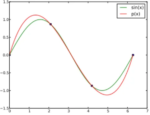
• 2.2.3
(1 point) Write a Python program that plots
numpy.sin()and its interpolating polynomial on the interval [0, 2π] (as in figure 1).
0 1 2 3 4 5 6 7
1.5 1.0 0.5 0.0 0.5 1.0
1.5 sin(x)
p(x)
Figure 1: sin(x) and the interpolating polynomial p(x) Task 2.3: Gauss Elimination and Pivoting (4 points)
• 2.3.1
(2 points) Extend the function
gauss_eliminate()from task 2.1 such that it implements the Gausselimination with partial pivoting (Spaltenpivotisierung). With this function, it should be possible to solve A
2x
2= b
2from Task 2.1.
• 2.3.2