Low Temperature Collisions and Reactions in a 22-Pole Ion Trap

Low Temperature Collisions and Reactions in a 22-Pole Ion Trap

Inaugural-Dissertation zur

Erlangung des Doktorgrades

der Mathematisch-Naturwissenschaftlichen Fakult¨ at der Universit¨ at zu K¨ oln

vorgelegt von Sven Fangh¨ anel

aus Gera

K¨ oln, 2018

Tag der m¨ undlichen Pr¨ ufung: 11.01.2018

When the Going Gets Tough, the Tough Get Going.

- Billy Ocean

- Oskar Asvany (15/11/17)

Die vorliegende Arbeit ist unterteilt in einen experimentellen und einen theoretischen Teil. Der experimentelle Teil befasst sich mit der Untersuchung von Ionen-Molek¨ ul Reaktionen in einem temperaturregelbaren 22 Pol Ionenspeicher. Im theoretischen Teil werden verschiedene Aspekte von Radio Frequenz Ionenspeichern und die Dy- namik von geladenen Teilchen in diesen analysiert.

Hierf¨ ur werden zun¨ achst in Kapitel 3 grundlegende Konzepte f¨ ur die Beschreibung von geladenen Teilchen in oszillierenden elektrischen Feldern erl¨ autert. Anschließend wird auf die Berechnung dieser Felder mittels verschiedener numerischer Verfahren eingegangen (Kapitel 4). Als besonders effiziente Methode zur Berechnung elektro- statischer Potenziale erwies sich die Randelemente Methode, die daher detailliert erl¨ autert wird. Mittels analytisch l¨ osbarer elektrostatischer Fragestellungen werden die zuvor numerisch berechneten Felder auf ihre Genauigkeit hin untersucht. F¨ ur die daf¨ ur notwendigen Berechnungen wurden sowohl eigene numerische Routinen entwickelt als auch bestehende Routinen verwendet. Es wird aufgezeigt, wie mit Hilfe einer geeigneten Multipolentwicklung die numerisch berechneten Felder in eine analytische Beschreibung ¨ uberf¨ uhrt werden k¨ onnen. Dies erm¨ oglicht eine effiziente Simulierung und Untersuchung der Dynamik von geladenen Teilchen in Ionenspe- ichern.

Mittels Simulationen verschiedener existierender Multipol Ionenspeicher (Kapitel 5) wird so das Verhalten von Ionen in elektrischen Wechselfeldern u.a. in Hinblick auf die Erh¨ ohung der Translationsenergie, die Energieverteilung und Verschiebungen der sekul¨ aren Oszillationsfrequenz durch h¨ ohere Anharmonizit¨ aten analysiert. Dar¨ uber hinaus werden Raumladungseffekte and St¨ orungen der Felder durch mechanische Fehljustierungen von Elektroden in die Analyse mit einbezogen. Damit leistet diese Arbeit einen Beitrag zur Optimierung bestehender sowie zur Entwicklung von neuen und besseren Ionenspeichern.

Im Fokus des experimentellen Teils steht die Reaktion von Stickstoffionen N

mit

Wasserstoffmolek¨ ulen H

unter Ber¨ ucksichtigung der Feinstrukturzust¨ ande der Stick-

stoffionen und der Kernspinzust¨ anden des Wasserstoffmolek¨ uls. Diese Reaktion

stellt den ersten Prozess bzw. die Vorstufe zur Bildung von interstellarem Am-

moniak dar. Trotz jahrzehntelanger Forschung ist diese fundamentale Reaktion bis

zum heutigen Tage nicht im Detail verstanden. So ist zum Beispiel offen, ob diese

Reaktion endotherm ist oder nur durch eine Barriere gehemmt wird. Weiter ist

ungekl¨ art inwieweit die Energie der Feinstrukturzust¨ ande der Stickstoffionen diese

Reaktion beg¨ unstigt. All diese Fragen sind von großer Relevanz f¨ ur die Astrochemie

bei tiefen Temperaturen. Zur Kl¨ arung dieser Fragen m¨ ochte diese Arbeit beitragen.

Unter Anwendung eines nicht adiabatischen Reaktionsmodells und einer globalen Anpassung an die gemessenen Daten werden feinstrukturspezifische Ratenkoeffizien- ten f¨ ur die oben genannte Reaktion bestimmt (Kapitel 7).

Zun¨ achst wurden hief¨ ur eine Vielzahl verschiedener Testmessungen durchgef¨ uhrt, um den Einfluss unterschiedlicher Messparameter wie z.B. der Temperatur oder der Teilchenzahldichte auf die gemessenen Ratenkoeffizienten hin zu untersuchen (Kapi- tel 6). Anhand dieser Testmessungen konnten m¨ ogliche Ursachen in Bezug auf die anf¨ anglich teils schlechte Reproduzierbarkeit von Messergebnissen identifiziert wer- den. Daraufhin wurden verschiedene Messabl¨ aufe optimiert, um den Fehler in den zu messenden Ratenkoeffizienten zu minimieren. Als Folge dieser Testmessungen wurden ebenfalls Ratenkoeffizienten f¨ ur die Reaktion von N

mit Wasserstoff in einem Temperaturbereich von 10 bis 120 K sowie tern¨ are Ratenkoeffizienten zur Bildung von Stickstoff-Helium Clustern (NHe

)

(n = 1, 2) bei Temperaturen zwis- chen 10 und 13 K bestimmt (Kapitel 9). Weiterhin wurden Messungen in Hinblick auf eine m¨ ogliche Umbesetzung der Feinstrukturzust¨ ande der Stickstoffionen durch St¨ oße mit Helium durchf¨ uhrt.

Dar¨ uberhinaus beinhaltet diese Arbeit die Charakterisierung eines piezo-elektrischen

Ventils (Kapitel 10). Diese wurde mittels der Reaktion von Argonionen mit Wasser-

stoffmolek¨ ulen durchgef¨ uhrt. Die Absicht dieser Charakterisierung ist es, die f¨ ur

Ionen-Molek¨ ul Reaktionen verwendete Messmethode weiter zu entwickeln. So soll

erm¨ oglicht werden, die translatorische Thermalisierung der Ionen sowie deren Re-

laxation intern angeregter Zust¨ ande, von der Reaktion zu trennen. Schlussendlich

konnte ein Modell entwickelt werden, welches den Reaktiongasfluss von Wasserstoff

als Funktion der Zeit, der Temperatur und des Reaktiongasdrucks beschreibt.

This work consists of two major parts, a theoretical and an experimental one. The latter part investigates ion molecule reactions performed in a temperature variable 22-pole ion trap. The former one analyses different aspects of radio frequency ion traps and the dynamics of charged particles located inside.

Therefore, fundamental concepts for the description of charged particles in oscil- lating electrical fields are discussed on as a first step (Chapter 3). The calculation of these fields via different numerical methods is elaborated on subsequently (Chap- ter 4). The boundary element method (BEM) has proven highly adequate for the calculation of electrostatic potentials. Hence it is depicted in detail. Using analyt- ically solvable electrostatic problems, the previously calculated fields will be tested with respect to their accuracy. To perform the necessary calculations both own numeric routines have been developed and available routines have been employed.

This work shows how the numerically, calculated fields can be converted into an analytical description

appropriate multipole expansion. This permits an effi- cient simulation and investigation of the dynamics of charged particles in ion traps.

Simulations of different existing multipole ion trap geometries help to analyze the behavior of ions in oscillating fields with respect to,

translational energy, their energy distribution and shifts of the secular frequency caused by higher anharmonicities (Chapter 5). Furthermore, space charge effects and perturbations of the fields due to mechanical misalignments of electrodes are included here. Consequently, this work is meant to contribute to the optimization of existing ion traps and to the development of new and better ones.

The experimental part focuses on the reaction of nitrogen ions with hydrogen molecules taking into account the fine structure state of N

and the nuclear-spin state of H

. This reaction can be considered as the first process or step in the formation of inter- stellar ammonia. Up to date this very fundamental reaction – although having been studied in several laboratories for decades – is not fully understood. For example, it remains unclear whether or not the reaction really endothermic or it is just inhibited by a barrier. Also, it is not known to what extent the fine structure state energy N

favours/promotes this reaction. All these questions are of great relevance for low temperature astrochemistry.

Applying a non-adiabatic reaction model and a global fit, fine structure state spe- cific rate coefficients for the reaction mentioned above could be derived (Chapter 7).

Initially, a large number of test measurements were conducted in order to clarify

the impact of different measurement parameters like e.g. temperature or number

density on measured rate coefficients (Chapter 6).

On the basis of these test measurements probable conclusions of initial difficulties with reproducing test results could be drawn. Thereupon, experimental processes were optimized to minimize errors in determination the rate coefficients. As a result, rate coefficients for the reaction of N

und CO

with hydrogen in a temperature range between 10 to 120 K were determined as well as ternary rate coefficients for the formation of nitrogen-helium-clusters (NHe

)

(n = 1, 2) in a temperature range between 10 – 13 K (Chapter 9). Also, measurements were performed with respect to fine structure state changing collisions of the nitrogen ion due to helium.

Moreover, this work contains the characterization of a piezoelectric valve which was

performed using the reaction of Ar

ions with H

(Chapter 10). The purpose of

the characterization is to develop a new experimental method for the study of ion

molecule reactions. This aims at separating translational thermalization of ions as

well as their relaxation of the internal excited states from the reaction process. A

quantitative model could be developed in order to describe the reaction gas flow as

a function of time, temperature and reaction gas pressure.

1 Introduction 1

2 Charged Particle Traps 3

2.1 Principle of Storing Charged Particles . . . . 3

2.2 The Poisson Equation . . . . 5

3 Motion of Ions in Oscillating Electric Fields 7

3.1 The Motion of Ions in an Ideal Quadrupole Field . . . . 7

3.2 The Motion of Ions in Inhomogeneous Fields . . . . 9

3.2.1 The Effective Potential Approximation . . . . 9

3.2.2 The Numerical Calculation of the Motion of Ions in Oscillating Fields . . . 14

3.3 The Stability Parameter

. . . 16

4 Methods for Calculations of Electrical Potentials of Ion Traps 18

4.1 Ideal Multipole Traps . . . 18

4.1.1 Two Dimensional Hyperbolic Shaped Multipole Traps . . . 19

4.1.2 Three Dimensional Hyperbolic Shaped Multipole Traps . . . . 19

4.2 The Calculation of Electric Fields for Arbitrary Geometries . . . 20

4.2.1 Numerical Methods for the Calculation of Electrical Fields . . 21

4.3 Multipole Expansions for Different Types of Ion Traps . . . 29

5 Simulations of Different Types of Ion Traps 31

5.1 Approximation of Hyperbolic Shaped Electrodes . . . 31

5.1.1 The Ideal Ratio

of a Linear Multipole Trap . . . 32

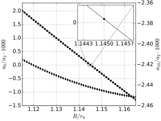
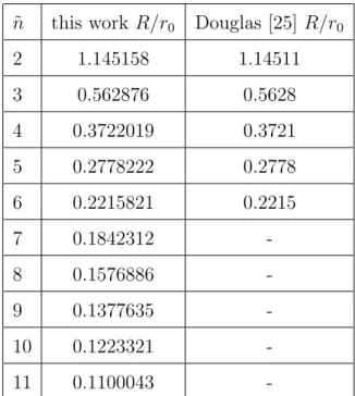
5.1.2 Influence of Higher Order Multipole Components on a Quadrupole 35 5.2 Influence of the Finite Size of Hyperbolic Electrodes . . . 41

5.3 The Split Ring Electrode Trap . . . 42

5.4 The 22 Pole Ion Trap . . . 49

5.4.1 The Kinetic Energy Distribution . . . 53

5.4.2 Mechanical Misalignments of the RF Electrodes . . . 61

5.5 A Linear 24 Pole Quadrupole Trap . . . 64

5.6 Space Charge Effects . . . 70

CONTENTS

6 Experimental Work 84

6.1 Experimental Setup and Techniques . . . 84

6.1.1 Determination of the Reaction Gas Density . . . 86

6.2 Time Evolution of Chemical Reactions . . . 87

6.3 Testing the LIRtrap Setup . . . 88

6.3.1 Tests to Improve the LIRtrap Setup . . . 90

7 N⁺

+

+

7.1 The N

(

P

) + H

(j) Reaction . . . 99

7.1.1 The Adiabatic Model . . . 100

7.1.2 The Non-Adiabatic Model . . . 103

7.1.3 Results . . . 114

8 The N⁺

+

9.1 (N−He

)

Cluster . . . 124

9.2 The Ternary Reaction of N

+ H

+ He

NH

+ He . . . 126

10 Characterization of a Piezoelectric Valve 132 11 Conclusion and Outlook 153

11.1 Experimental Part . . . 153

11.2 Theoretical Part . . . 154

A Appendix 164

A.1 Approximation of Hyperbolic Shaped Electrodes . . . 164

A.2 Space Charge Effects . . . 166

A.3 Tests to Improve the LIRtrap Setup . . . 166

A.3.1 The Stability of Guiding and Trapping the Ions . . . 166

A.3.2 Saturation Effects of the Ion Detection System . . . 168

A.3.3 Temperature Behavior of the Reaction Gas Calibration and the N

+ H

Reaction . . . 172

A.3.4 The Number Density of the Reaction Gas at Low Temperatures177 A.3.5 Measuring Rate Coefficients during the Cool Down Phase of the Apparatus . . . 179

A.3.6 Steady State of the Apparatus . . . 180

A.3.7 Improving the Measurement Procedure . . . 181

A.4 The N

(

P

) + H

(j) Reaction . . . 185

A.4.1 A Simple Approach for the Analysis of Reaction N

+ H

(j) . . . 185

A.5 The Ternary Reaction of

N

+ H

+ He

NH

+ He . . . 188

A.6 Characterization of a Piezoelectric Valve . . . 190

Danksagung . . . 192

Lebenslauf . . . 194

Chapter 1 Introduction

Star-formation processes, starting with the collapse of a dense cloud ending with the dying of a star, are the major topics in astrophysics and is ultimately related to the question of the formation of our own solar system and the origin of life on earth. To gain insight into star formation, electromagnetic radiation is the main source of information on the structure and properties of cosmological objects. Here, the interstellar medium (ISM) plays an important role. The temporal evolution of the ISM is determined and accompanied to a large degree by the chemistry and the formation of small molecules in the gas phase. In order to understand gas phase processes, the knowledge of chemical reaction rate coefficients is of fundamental importance. These rate coefficients are used in astronomical network models to calculate molecular abundances, the age of an object or to predict or model the dynamics of interstellar clouds. Ion-molecule reactions are very efficient at very low temperatures in the ISM as many of such reactions have no or low activation energies. Initially, ionization is driven by cosmic rays (high-energy

protons) H

+ cosmic rays

H

+

or photo-ionization H + hν

H

+

followed by fundamental reactions such as:

H

+ H

H

+ H (1.1)

H

+ M

MH

+ H

(M denotes an atom or molecule) (1.2)

N

+ H

NH

+ H (1.3)

that are the key to the synthesis of more complex molecules in the following. In this respect, rate coefficients of ion-molecule reactions are of fundamental importance for the quantitative understanding of the chemistry in the ISM.

Ion-molecule reactions and their rate coefficients are not only relevant for the insight

into astronomical processes but they also play an important role for the chemistry

in the ionosphere of the earth (altitude

100 km). The main source of ionization

is the photo-ionization by solar ultraviolet light or by cosmic rays

. For example,

since electrons are able to reflect electromagnetic waves, the electron density in the

ionosphere is of practical relevance for the transmission of radio waves. This electron

density is determined by the balance between the ionization of atoms and dissocia-

tive recombination of ions with free electrons. This equilibrium is mainly governed by the ion-molecule rate coefficients

.

This thesis is divided in two parts, a theoretical and an experimental one. The experimental part is focused on the investigations of astrophysical relevant ion- molecule reactions in a temperature variable 22-pole ion trap apparatus. Here spe- cial attention is payed to the reaction of the N

with molecular hydrogen under the consideration of the fine structure population of the nitrogen ion in dependence of the nuclear spin configuration of H

. This fundamental reaction, which is the first step in the reaction chain to form interstellar ammonia has been investigated by sev- eral groups over the last three decades remains is not well understood until today.

Here, the role of the energy provided by the fine structure of the nitrogen ion in promoting this reaction is rather unclear whereas the role of the energy dependence on the nuclear spin configuration of the hydrogen molecule is largely understood.

To allow precise predictions of the chemical evolution of ammonia a detailed un- derstanding of this reaction mechanism is required. Therefore fine structure specific rate coefficients for this reaction are of great astrophysical interest. A further aspect which makes the reaction so interesting is, that this system is very sensitive to the nuclear spin configuration (ortho/para) of the hydrogen molecule and can therefore be used to investigate the purity of an para hydrogen sample.

The theoretical part covers different aspects of trapping charged particles. Among

others, different methods to describe the dynamics of charged particles in inhomoge-

neous oscillating electric fields will be given. In this context also different methods

for the calculation of such electric fields will be presented. Here, especially the

boundary element method and their accuracy is described in detail. Based on simu-

lations of various existing radio frequency trapping devices, it will be demonstrated

to what extent such calculations can help to understand the behavior of ions in os-

cillating electric fields and to develop new or to optimize existing trapping devices.

Chapter 2

Charged Particle Traps

Charged particle traps are a powerful tool to investigate the dynamics of charged particles and which are used nowadays in various scientific and commercial appli- cations. Different types of such traps are used e.g. for spectroscopic investigations of ions, for the determination of rate coefficients of chemical reactions or for the measuring and manipulation of quantum systems which may be used for the devel- opment of quantum computers.

The development of trapping charged particles in such devices was expedited by W.Paul

and H.G.Dehmelt

who got the Nobel prize in Physics 1989 ’for the de- velopment of the ion trap technique’. A comprehensive historical overview about storing charged particles can be found in Refs.[5, 6].

The idea of a charged particle trap is to confine or control the trajectories of positive or negative charged particles, using electromagnetic fields. In general, such instru- ments consist of electrodes to which voltages are applied surround a certain volume (see Fig. 2.1). A detailed description of storing charged particles will be given in the following sections.

2.1 Principle of Storing Charged Particles

In general electromagnetic fields are used to store, guide or mass select positive or negative charged particles. The Lorentz force

influences the trajectories

charged particles in an external electric or magnetic field.

m¨r

=

=

+

(2.1)

Here is

the electric field,

the magnetic field,

= ˙

is the velocity and

respectively

are the charge and the mass of the particle. In the following sections only electrical radio frequency (rf) trapping devices will be discussed (B = 0,

A good overview about many kinds of charged particle traps is given in the book of

Major,Gheorghe and Werth

.

Vdc+Vrf⋅cos(Ωt)

Figure 2.1: The sketch shows a possible electrode configuration of a charged particle trap (http:

//www.spektrum.de/lexikon/physik/atom-und-ionenfallen/885).

A consequence of the ’Earnshaw theorem’ is, that it is not possible to store charged particles in static electric fields. One option to avoid this problem is the periodic change of the polarity of an electric field with an angular frequency Ω (see Fig. 2.1) which will result in an oscillating motion of the particle.

In order to describe the behavior or the motion of charged particles in electric trapping devices (ion traps), the knowledge on the driving electric field

necessary. Here the electric field

can be calculated from the Maxwell equations.

A simplification of the problem is, that one may calculate the electric field in the quasielectrostatic limit

of

Ω

c

1. (2.2)

Here Ω is the angular frequency of the time varying field,

the length of the device in which the field changes and

the speed of light. Typical values for an ion trap are

= 0.01

and Ω = 100

which leads to:

Ω

c

= 100M Hz

0.01m

3

10

= 0.0033 1.

As a consequence time dependent propagation of electromagnetic waves can be ne- glected resulting on a separation of the electric field in an oscillating part with an angular frequency Ω and a static part.

E(r, t) = cos(Ωt)·E(r)

(2.3) Since

=

=

0

with

the space

charge, the whole problem reduces to the Poisson equation.

2.2 The Poisson Equation 5

2.2 The Poisson Equation

In general a static electric field

are determined by the size, the alignment, the geometry and the applied voltage of its electrodes. Assuming no space charge effects induced by charge particles, the problem of finding the electrostatic potential Φ reduces to the ’Laplace-equation’

with Dirichlet boundary conditions

∆Φ = 0 with Φ

on boundary (2.4)

with being Φ

the applied voltage on the electrodes. If one have a relevant amount of charged particles between the electrodes then space charge has taken into account and the electrostatic potential Φ is governed by the ’Poisson-equation’

∆Φ =

₀

with Φ

on boundary,, (2.5)

where denotes

The effect of space charge will be discussed in section 5.6. Hence

E

=

=

(2.6) a possible solution for

or

can be found by integrating Eq. 2.6.

E(x, y, z) = axe_x

+

+

(2.7) If the constants

are set to

=

=

= 4 the electrostatic potential Φ fulfill the Laplace equation (Eq. 2.4).

Φ(x, y, z) =

+

2z

(2.8) To find the shape of the boundary (the geometry of the electrodes) which fulfills Eq. 2.4 one has to set Φ = Φ

. For simplicity one may also set

= 0 leading to

=

. The latter describes equipotential lines with a hyperbolic shape. This implies only infinitively long hyperbolic shaped electrodes have the correct boundary conditions to fulfill the Laplace Equation. If one chooses

=

x²₀

+

, which is the shortest distance to the electrodes in radial direction, and divide Eq. 2.8 by the constant factor of 2r

than Eq. 2.8 results in:

Φ(x, y, z) =

+ 2z

2r

(2.9)

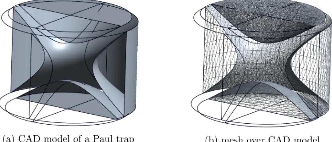
This theoretical example is known as the so called spherical or 3 dimensional ’Paul Trap’, which is named after its inventor Wolfgang Paul

. This kind of ion trap consists of two hyperbolic shaped ’endcap’ electrodes with a distance to the center of

=

2

and a hyperbolic shaped ring electrode with a distance to the center of

(see Fig. 4.2a). Setting the constants

=

=

= 0 in Eq. 2.7 will also

result in a possible solution for the 2 dimensional Laplace equation which is known as the electric potential of the rf part of a linear quadrupol mass filter (QMF) (see Fig. 2.2).

Φ(x, y) =

r²₀ .

(2.10)

These two analytic solutions for the electrostatic potentials are only valid if one assumes infinitively long hyperbolic shaped electrodes. Multiplying Φ by a time varying factor

cos(Ωt), with

being its amplitude , Eq. 2.11 will represent the time varying electric potential.

Φ(r, t) =

cos(Ωt)

Φ(r) (2.11) The time varying electric field can be calculated as follows:

E(r, t) =−Vrf

cos(Ωt)∇Φ(r). (2.12)

-0.800 -0.800

-0.400

-0.400

-0.100 -0.100

0.100

0.100

0.400

0.400

0.800 0.800

-0.9 -0.7 -0.4 -0.2 0.0 0.2 0.4 0.7 0.9

Figure 2.2: The plot shows the electrostatic potential of a QMF (eq. 2.10) produced by hyperbolic electrodes. The thick black lines indicate the boundary of the hyperbolic electrodes.

Some other analytic solutions for special trap geometries can be found in Ref.[5].

Chapter 3

Motion of Ions in Oscillating Electric Fields

In order to describe the motion of ions, one can make use of Newtons Equations of Motion (EoM). Using Newtons law

=

=

is the elemetary charge and

is the mass, the motion of ions in time varing electric fields can be described with the classical equation of motion.

¨

r(t) = e

m ·E(r(t), t) = −e

m · ∇Φ(r(t), t)

(3.1) In general it is not possible to find an analytically solution of this equation because it is a highly coupled second order differential equation. Only for some special field geometries Φ it is possible to calculate the motion of the ions analytically.

3.1 The Motion of Ions in an Ideal Quadrupole Field

An ideal oscillating quadrupole field can be described by Eq. 2.11. Additionally, this field can be superimposed by a static potential

, which will be defined as follows:

Φ(r, t) = (V

cos(Ωt))

(3.2) Here, Eq. 2.11 describes only a guiding field for the ions. The static field

lead to an additional drift which can be used to select ions by their charge to mass ratio.

This means, for certain values of

only ions with a specific charge to mass ratio will have stable trajectories in an ideal quadrupole field. For such ideal quadrupole fields an analytic description of stable ion trajectories is possible. With equations. 3.2 and 2.12 the Equations of Motions for a QMF (Eq. 2.10) are:

¨

x(t) =−

2e

mr₀²

(V

cos(Ωt))

¨

y(t) =

2e

mr²₀

(V

cos(Ωt))

(3.3)

This is a system of second order decoupled time dependent differential equations.

Given the following substitution

=

,q

=

,

=

,q

=

and

=

one can rewrite Eq. 3.3 such as:

d²u(ξ)

dξ²

=

(a

2q

cos(2ξ))

(3.4) with

= (x, y). These differential equations are known as the ’Mathieu Differential Equation’. Using ’Floquets-Theorem’, the solution of Eq. 3.3 have the following form [6]:

u(t) =Ae^iωutX

n

C_2ne^inΩt

+

n

C_2ne^−inΩt

(3.5) Here

=

.

depends on the substituted parameters in the Mathieu equation

and

. The solutions are stable for 0

1. A more detailed description of these procedure can be found in Refs. [6, 9]. For each direction (x, y) one will find regions of stability in the

plane. The overlap of both regions defines the stability region or so-called stability diagram. Figure 3.1 shows the stability diagram of the first stable region of a QMF.

0.0 0.2 0.4 0.6 0.8 1.0

q

0.00 0.05 0.10 0.15 0.20 0.25

a

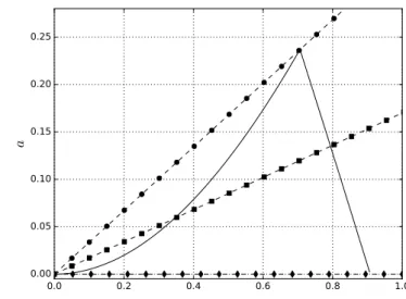
Figure 3.1: The plot shows the stability diagram of the first stability region of a QMF. The solid lines indicate the boundaries of the stable region. The dashed lines illustrate the different operation modes of a QMF. The circles, squares and diamonds represent different masses, where high masses are more left (from q = 0 ) and low masses come from the right side of the plot. In practice a fixed angular frequency Ω is chosen. To receive a mass-spectrum the QMF will operated with a so-called load line or working line which is defined as the ratio ofa/q(withaandqdefined above).

IfV_dc= 0 (diamonds) the QMF will work as a high-pass which means all masses about a critical mass can pass the QMF. If the slope is exactly V_dc/V_rf = ¹₂ · ^a_q = ¹₂ · ^0.23699_0.706 (the point which define the top of the stability triangle) the QMF will select to pass through only one mass (circle on the top of the stability triangle). For amplitudes 0< Vdc/Vrf <¹₂·^0.23699_0.706 all masses (squares) in between the stability triangle will pass the QMF.

3.2 The Motion of Ions in Inhomogeneous Fields 9

Generally there are more than one stability regions. For practical reasons ion traps are operated in the first stable region to avoid exceedingly high values of the angular frequency Ω and the amplitudes of

and

.

3.2 The Motion of Ions in Inhomogeneous Fields

As mentioned before, it is not possible to find in general analytical solutions to the EoM’s because they are nonlinear coupled second order differential equations. One approach is to calculate the trajectories with numerical integration routines or to describe the motion within the so called effective potential approximation

. In the following a mathematically description of the motion of an ion using the effective potential approximation will be given.

3.2.1 The Effective Potential Approximation

Due to the superposition principle of electric fields, the motion of a charged particle can be described by the following differential equation:

m

e

¨

=

(r) cos(Ωt) +

(r) (3.6) with

(r) being the time varying part and

(r) the electrostatic component of the electric field. If one assume that one can superimpose the solution

as smooth drift motion

and a fast oscillating motion

(see Fig. 3.7), one can write

as:

r(t) = R₀

(t) +

(t) =

(t)

(3.7) where

of the electric field at the position

(t) . Furthermore one may assume a small spatial variation of

(t)

E(R₀

(t)

(R

) cos(Ωt)

(R

)

(Ωt)

+

(R

)

(R

)

(3.8) where

is the Jacobian matrix of the static and the radio frequency electric field. Utilizing the notation

i

=

the Jacobian matrix of an electric field

= (E

) is defined as follows:

J_E

= [∂

] (3.9)

Substituting Eq. 3.8 in Eq. 3.6 leads to the following equation.

m·

( ¨

(t)

dt²

(a(t) cos(Ωt))) =

(R

) cos(Ωt)

(R

)

(Ωt) +

(R

)

(R

)

(3.10)

1Also known as the adiabatic approximation.

with

dt²

(a(t) cos(Ωt)) =

cos(Ωt)

Ω

¨

2 ˙

(3.11) If the angular frequency Ω is large and one have slow variation of the amplitude of the fast oscillating motion

Ωa, ˙

Ω

and also ¨

Ω

one can neglect the last two terms in Eq. 3.11.

d²

dt²

(a(t) cos(Ωt))

(3.12) Furthermore assuming that

one can write

a(R₀

) =

(R

)

mΩ²

(3.13)

The time dependent fast oscillating term can now be written as:

R₁

(t) =

(R

)

mΩ² ·

cos(Ωt) (3.14)

Substituting the latter in Eq. 3.10 will lead to:

m·R

¨

(t) +

(R

) cos(Ωt) =

(R

) cos(Ωt)

− e²

mΩ²J_Erf

(R

)

(R

) cos

(Ωt) +

(R

)

mΩ²J_Est

(R

)

(R

) cos(Ωt) (3.15) If one write

as the negative gradient of the electric potential

=

Schwarz’s theorem

, one may simplify

to

JE·E

= 1

2

(3.16)

Canceling out the two equal terms on the left and right side of Eq. 3.15 leads to:

m·R

¨

(t) =

2mΩ

(R

) cos

(Ωt) +

(R

)

mΩ²J_Est

(R

)

(R

) cos(Ωt)

(3.17)

Averaging Eq. 3.17 with respect to time,

(Ωt)i

becomes

and

be- comes 0. This leads to a differential equation for the smooth drift motion

without an oscillating part. Replacing

(R

) by

(R

), the time average of Eq. 3.17 is:

m·R

¨

=

4mΩ

(R

)

(R

) (3.18)

3.2 The Motion of Ions in Inhomogeneous Fields 11

If one set

V^∗

(R

) =

(R

)

4mΩ

+

(R

), (3.19)

the ion motion can be described by a time independent potential

. The equation of motion for the secular motion or macro motion

can be written as:

m·R

¨

=

(R

) (3.20)

The potential

has different names like the effective potential, pseudo potential, ponderomotive potential or high frequency potential. If one integrate Eq. 3.20 with respect to time one obtain the following expression

1

2

˙

+

(R

)

4mΩ

+

(R

) =

(3.21) Hence, in the limit of the adiabatic approximation the energy is a constant which can be converted from the kinetic energy of the macro motion into the effective potential energy. It is straight forward to see that the second term in Eq. 3.21 is the same as the time average of the kinetic energy of the fast oscillating motion

(t) and also similar to the radio frequency part of the effective potential

.

h

1

2

˙

=

(R

)

2mΩ

sin

(Ωt)i =

(R

)

4mΩ

(3.22)

This proves: ”The motion through an inhomogeneous field leads to a permanent exchange between three different forms of energy, the kinetic energies,

˙

and

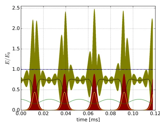
1

2mR

˙

and the electrostatic potential energy

” (Gerlich

, p. 14). Figures 3.4

and 3.5 show the different forms of energies of an ion moving in a real 22-pole

trap. The validity of this approximation can be proven by integrating Eq. 3.20

and superimposing this motion with the fast oscillating motion, Eq. 3.14. Figures

3.2 and 3.3 show a comparison of the full numerical calculated trajectories of an ion

moving in 22-pole trap with a superimposed static electric field

(V

= 1.5V ) and

the trajectories calculated within the adiabatic approximation. For demonstration

purposes the stability parameter

)

was chosen to be 0.28 at the edge of the

stability region. The meaning of the stability parameter

the next section 3.3.

0.8 0.6 0.4 0.2 0.0 0.2 0.4 0.6 0.8 x/r

0.8 0.6 0.4 0.2 0.0 0.2 0.4 0.6 0.8

y/ r

Figure 3.2: The plot shows a comparison of the numerically calculated trajectories (black) of an ion moving in a 22-pole trap with a superimposed static electric fieldEst (Vdc= 1.5V,η(R0) = 0.28) and the trajectories calculated within the effective potential approximation (green). The dashed line in the zoom marks the trajectories of the macro motion.

0.050 0.055 0.060 0.065 0.070 0.075 0.080 0.085 0.090 0.095 time [ms]

0.0 0.5 1.0 1.5 2.0 2.5 3.0 3.5

E /

E

Figure 3.3: The plot shows a comparison of the numerically calculated kinetic energy (black) of an ion moving in a 22-pole trap with a superimposed static electric field E_st (V_dc = 1.5V, η(R0) = 0.28) and the kinetic energy calculated within the adiabatic approximation (green). The dashed line marks the kinetic energy of the macro motion.

3.2 The Motion of Ions in Inhomogeneous Fields 13

For reasons of completeness the phase dependent initial energy can be expressed in the following form.

E₀

= 1

2

(t = 0) + ˙

(t = 0)]

+

(R

(t = 0))

4mΩ

+

(R

(t = 0)) (3.23) The dependence of the initial phase

can be taken into account if one sets

R

˙

(t) =

(R

)

mΩ ·

sin(Ωt +

(3.24)

For

= 0 Eq. 3.23 will lead to Eq. 3.21.

Figures 3.4 and 3.5 illustrate that the total time averaged energy (Eq. 3.25) of the ion motion is a constant.

hE_total

(t)i =

1

2

(t) + ˙

(t)]

+

(R

(t))i =

(3.25)

0.00 0.02 0.04 0.06 0.08 0.10 0.12

time [ms]

0.0 0.5 1.0 1.5 2.0 2.5

E /E

Figure 3.4: The plot shows the different forms of energies for an ion moving in a real 22-pole trap (Vdc= 1.5V,η(R0) = 0.28) as a function of the time. The green line shows the potential energy of the static electric fieldEst(R0(t)). The yellow line illustrates the energy from the rf-part of the effective potential V_rf^∗(R₀(t)). The solid black line shows the energy of the macro motion ˙R₀(t) and the red line from the micro motion ˙R1(t). The dashed black line shows the sum of the potential energy from the static electric field , the energy from the rf-part of the effective potential and the energy from the macro motion. This sum confirms Eq.3.21. The olive colored line shows the sum of the energy from the macro and micro motion. The blue line (behind the the black dashed line) shows the cumulative time average h¹₂m[ ˙R0(t) + ˙R1(t)]²+eΦst(R0(t))i

.

0.000 0.002 0.004 0.006 0.008 0.010 0.012 0.014 time [ms]

0.0 0.5 1.0 1.5 2.0

E /E 0

Figure 3.5: The plot shows a zoom for the first time interval of Figure 3.4. The blue line, the cumulative time averageh¹₂m[ ˙R₀(t) + ˙R₁(t)]²+eΦ_st(R₀(t))i reach a stable value after a few rf- periods. This nicely illustrates, that the mean total energy is conserved.

3.2.2 The Numerical Calculation of the Motion of Ions in Oscillating Fields

To investigate the consequences of non ideal fields to the ion motion inside an ion

trap one has to observe and evaluate the trajectories of the ions. This can also be

done by calculating the trajectories of ions moving in inhomogeneous fields with

numerical methods. From such calculations one gets an explicit impression of the

behavior (micro and macro-motion) of ions in an oscillating electrical field. Ad-

ditionally collisions with a background gas inside a trap or space charge effects,

which arise from the coulomb repulsion of an ion cloud can be included and eval-

uated statistically in such simulations. For this purpose the Equations of Motions

(Eq. 3.1) have to be solved numerically. In order to do so one has to integrate these

equations twice in time. This can be done with different numerical integration algo-

rithms like the Euler method or Runge Kutta methods (for example, Ref. [11]). To

solve second order differential equations there are special numeric algorithms like

the Nystrom-Kutta method. For all the numerical calculations of trajectories in this

thesis the Runge-Kutta-Nystroem-method

of fourth order, with a fixed step size

of

=

3.2 The Motion of Ions in Inhomogeneous Fields 15

ical solution of an ideal quadrupole (see Sec. 3.1) to ensure that the step size is small enough to be sensitive to small perturbations of Φ(r(t), t). Figures 3.6 and 3.7 show the comparison for trajectories calculated with the Runge-Kutta-Nystroem-method and the analytical solution, derived by mathematica, for

= 0.23651 and

= 0.706 and initial values of (x

) = (0.1

cos(

0.1

sin(

(u

) = (0, 0). The comparison shows, that a step size of

=

for numerical calculations of ion trajectories.

0 50 100 150 200 250 300 350 400

ξ

4 2 0 2 4 6 8

Figure 3.6: The plot shows the comparison of the analytic (black dots) and numeric (green line) solution for the trajectory forx(ξ).

0 50 100 150 200 250 300 350 400

ξ

0.04 0.02 0.00 0.02 0.04 0.06 0.08

Figure 3.7: The plot shows the comparison of the analytic (black dots) and numeric (green line) solution for the trajectory fory(ξ).

3.3 The Stability Parameter η

As mentioned above, regions of stability as a function of the parameters

can only be given for the special case of a quadrupole field. This is based on the fact, to best of my knowledge, that no analytical solutions of the equation of motions for oscillating inhomogeneous fields (eq. 3.1) are available. One possibility to find regions of stability for higher order multipole traps is to simulate numerical trajec- tories as a function of their initial conditions. This was done by H¨ agg and Szabo

for the transmission of a hexapole and octopol. Due to the enormous amount of initial parameters such an approach lead to a huge numerical effort. To evaluate the influence of inhomogeneities of the field to the stable ion motion, such an effort has to be done for each individual trap design.

A different approach is to evaluate the stability in the adiabatic approach of the effective potential approximation. Gerlich

introduced a dimensionless stability parameter

η(r) = |

2e

mΩ²∇|E(r)||

(3.26) Gerlich

gives a heuristic criterion

0.3 for save or stable operations in an ion trap. In general

is a scalar function of the spatial coordinate

(see Fig. 3.8).

Another approach is to compare the force of the trapping field

|F_trap

(r)| =

(3.27)

to the force of the effective potential.

|Fef f ective

(r)| =

(r)| ∝ |2|E(r)|∇|E(r)|| (3.28)

The ratio of Eq.3.28 and 3.27 lead to a parameter which is proportional to

|Fef f ective

(r)|

|F_trap

(r)| = 1

4

(3.29)

In case of a 2 dimensional quadrupol field Eq.2.10 the parameter

is identical with

the rf-parameter

in the Mathieu equation 3.4.

3.3 The Stability Parameter η 17

0.0 0.2 0.4 0.6 0.8 1.0

r/r 0 1.0

0.5 0.0 0.5 1.0

z/ r 0 0.100

0.200 0.300

0.500

1.000 1.000

0.00 0.18 0.36 0.54 0.72 0.90 1.08 1.26 1.44 1.62

Figure 3.8: The plot shows theη-map for a spherical octopol with the rf voltageV = 400 V , the mass m= 100 [amu] and the frequencyf = 2 Mhz. The solid lines indicate different values ofη for a given set of trapping parametersV, m, andf. It can be seen thatη ≤0.3 is valid for radii .40% ofr₀.

Methods for Calculations of

Electrical Potentials of Ion Traps

In this chapter an overview will be given about methods for the calculations of electric potentials. First, the electric potentials of a linear quadrupole mass filter (QMF) and spherical quadrupole (Paul-Trap) will be discussed. Furthermore, it will be demonstrated how to calculate numerically electric potentials for arbitrary trap geometries. Also a short overview about the different numerical methods for such calculations will be given. Especially the Boundary Element Method and its accuracy based on examples will be discussed in detail. Following this, it will be shown how these numerical solutions can be transfered in an analytical expression based on an appropriate multi-pole expansions.

As mentioned in chapter 2.1, the electrical potential Φ has to fulfill the Laplace equation. A general solution of the Laplace equation 2.4 in spherical coordinates is represented by the following expansion:

Φ(r, θ, φ) =

∞

X

l=0 l

X

m=0

cm,l

r r₀

l

(Y

(θ, φ))

(4.1) Here

are the multipole coefficients of order

the distance from the origin,

the normalized lenght, and

Y_m,l

=

(cos(θ))e

(4.2)

the spherical harmonics and

the associated Legendre polynomials. With this expansion it is possible to give simple formulas for ideal multipole traps. (More practicable formulas can be found in many textbooks Ref.[5–7, 14]).

4.1 Ideal Multipole Traps

A theoretical, ideal multipole trap consists of perfectly shaped and infinitively long

conductors. The shape of these conductors has to fulfill the boundary conditions

4.1 Ideal Multipole Traps 19

of the Laplace equation 2.4. Following Eq. 4.1 the shape can be derived for a fixed order

lines at a fixed potential Φ

.

Φ

=

r₀ n

P_n^l

(cos(θ))e

(4.3)

Φ

describes the shape of conductors (electrodes) of the multipole trap. For certain symmetries and dimensions Eq. 4.1 can be simplified.

4.1.1 Two Dimensional Hyperbolic Shaped Multipole Traps

Assuming infinitely long conductors as electrodes, the

dependence of the electric potential can be neglected and Eq. 4.1 reduces in polar coordinates to

Φ(r, φ) =

∞

X

n=0

r r₀

n

(a

cos(nφ) +

sin(nφ)) (4.4) where

are the symmetric and antisymmetric expansion coefficients and

is the closest distance from the center of the trap to the electrode surface (normalized length). The electric field

=

of two dimensional multipole traps in polar coordinates can be written as:

E

=

∂r

Φ(r), 1

∂

∂φ

Φ(r)

(4.5)

=

∞

X

n=1

n r₀

r r₀

n−1

[−(a

cos(nφ) +

sin(nφ)), (a

sin(nφ)

cos(nφ))]

or in Cartesian coordinates:

(E

) =

∞

X

n=1

n r₀

r r₀

n−1

[−(a

cos(˜

sin(˜

(a

sin(˜

cos(˜

with ˜

=

1. For

= 2 and a symmetric alignment of the electrodes Eq. 4.4 reduces to

Φ(r, φ) =

r₀ 2

cos(2φ) =

r₀² .

(4.6)

This equation represents the quadrupole potential with hyperbolic shaped surfaces as electrodes (see Fig. 2.2).

4.1.2 Three Dimensional Hyperbolic Shaped Multipole Traps

If one assumes some symmetry with respect to the z-axis, this induces an indepen- dence on the angle

Φ(r, θ) =

∞

X

n=0

c_n r

r₀ n

P_n

(cos(θ)) (4.7)

where

(cos(θ)) are the Legendre polynomials of order

with respect to the angle

and

is the distance from the center of the trap to the electrode surface. For

= 2 and

= 1 Φ reduces to

Φ(r, θ) =

r₀ 2

P₂

(cos(θ)) =

+ 2z

2r

(4.8)

the electric potential of time varying part (Φ

) of a spherical Paul-Trap (see Eq. 2.9).

It is clearly visible, that the description for the two and three dimensional case is only valid under the assumption of hyperbolic shaped and infinitely long electrodes.

For real trap geometries other methods have to be applied in order to solve for the electric potential.

4.2 The Calculation of Electric Fields for Arbi- trary Geometries

In this section, different numerical methods to calculate electrical potentials will be highlighted. Advantages and disadvantages of different numerical methods will be shown. A short mathematical introduction to the Boundary Element Method (BEM) will be given. In addition, the accuracy of the calculated solutions with BEM will be discussed in detail based on three examples. Also the benefit of the description of the solutions via an appropriate multipole expansion will be explained based on real existing examples.

Due to the superposition principle, the electrical field of an ion trap can be repre- sented by a time dependent oscillating part

(r, t) and static part

(r) which leads into

E(r, t) = E_rf

(r, t) +

(r) = cos(ωt +

(r) +

(r) (4.9) With Eq. 2.6 the electric potential Φ can be expressed by:

Φ(r, t) = Φ

(r, t) + Φ

(r) = cos(ωt +

Φ

(r) + Φ

(r) (4.10) where

is an arbitrary phase. To separate the oscillating

part from the static part of the field two cases must be calculated:

1. cos(ωt

+

Φ

(r, t

) 2. cos(ωt

+

Φ

(r, t

)

The addition and subtraction of these cases results into the static and oscillating part of the field.

=

Φ

(r) = 1

2

(Φ

+ Φ

) and Φ

(r) = 1

2

(Φ

Φ

) (4.11)

4.2 The Calculation of Electric Fields for Arbitrary Geometries 21

4.2.1 Numerical Methods for the Calculation of Electrical Fields

For two dimensional problems like the electric potential

of a QMF with circular electrodes instead of hyperbolic shaped ones, it is possible to calculate the electric potential with semi analytical methods. Under the assumption of an infinite length and use of complex analysis it is possible to calculate the electric potential with a so called conformal mapping

.

To the best of my knowledge, for real traps with a finite geometry, there are no analytic solutions available. Therefore one has to calculate the potential numerically.

There are several methods to do this. The main idea is the discretization of the continuous problem and the conversion into a system of linear equations. The most popular methods are:

1. the finite difference method (FDM) 2. the finite element method (FEM) 3. the boundary element method (BEM)

There is a lot of commercial software (Simion

, Comsol

, CPO

, Integrated

...) available which using the different methods.

The FDM method makes use of the Taylor theorem to approximate the solution applying the central difference method on a grid

. This gives a

system of linear equations for a one dimensional problem with

grid points.

The FEM also discretizes the space where the solution is required. The problem is disassembled on a grid in so called ansatzfunctions. With a linear combination of these ansatzfunctions one gets an approximated solution of the problem

.

The BEM method makes use of Greens second identity to reformulate the problem in an integral equation. This will be explained in more detail in the following section.

The first two methods (FDM, FEM) have major disadvantages compared to the BEM method. For the formulation of the numeric problem one has to discretisize the complete space, i.e. the electrodes and the space between the electrodes. For calculations with high accuracy (especially for three dimensional problems) this will lead to a tremendous pc-memory effort. Another disadvantage is that one can calculate the solution only on given grid points. For points inbetween one has to interpolate which leads to numerical errors. A further problem of these two methods are that discretized space is finite, leading to the question: What are the right boundary conditions? However, the advantage of these two methods is that it allows for solving a huge amount of linear and nonlinear problems in physics and engineering. Furthermore, these methods are mathematically simpler (less computationally demanding) to implement in numeric algorithms.

1http://simion.com/

2https://www.comsol.de/

3http://simion.com/cpo/

4https://www.integratedsoft.com/

The Boundary Element Method

In difference to the FDM and FEM, the BEM needs only a discretization of the boundary. Actually this is the reason for the name of the method. In the case of electrostatic problems, only the surface of the electrodes needs to be discretized.

Therefore the problem is reduced by one dimension (the surface of a three dimen- sional manifold is two dimensional).

As mentioned before, the BEM method make use of Green’s second identity

. This allows to write the solution Φ (x) for a

Ω

as an integral equation

,

Φ(x)η(x) =

Γ

g

(x,

∂n

Φ (y)

Γ

∂

∂ng

(x,

(4.12)

Ω,

Γ with Γ a smooth boundary (surface of the electrodes), Φ (y) (the applied voltage at the electrodes) and

η(x) =







0 if

inside the electrodes 1 if

outside the electrodes

1

2

if

on the electrodes.

(4.13)

∂

∂n

=

+n

+n

denotes the normal derivative and

(x,

solution for the Laplace problem for

= 2, 3.

g

(x,

(−_2π¹

ln

= 2

1

4π|x−y| , n

= 3. (4.14)

For electrostatic problems Eq. 4.12 can be simplified. In electrostatic problems electrodes one held on a fixed potential. Therefore Φ(y) = Φ

is a constant for each electrode. This corresponds to the so called exterior Dirichlet problem. The only unknown in Eq. 4.12 is

Φ(y) which is proportional to the surface charge density

. The first and second integral on the right side of Eq. 4.12 are often denoted as single and double layer potential operators.

S(x) = I

Γ

g

(x,

∂n

Φ (y)

(4.15)

D(x) = I

Γ

∂

∂ng

(x,

(4.16) One can show, that in the case of a fixed potential (Φ

=

at each electrode) the double layer potential

:

D(x) =







0 if

outside the electrodes Φ

if

inside the electrodes

Φ0

2

if

on the electrodes

(4.17)