Morning aerosol vertical profiles in the Planetary Boundary Layer: Observations on a Zeppelin NT Airship and comparison with a Regional Model

Morning aerosol vertical profiles in the Planetary Boundary Layer:

Observations on a Zeppelin NT Airship and comparison with a Regional Model

INAUGURAL-DISSERTATION

zur

Erlangung des Doktorgrades

der Mathematisch-Naturwissenchaftlichen Fakult¨ at der Universit¨ at zu K¨ oln

vorgelegt von

Konstantinos Kazanas aus Athen, Griechenland

K¨ oln 2017

ii

Berichterstatter: Prof. Dr. Andreas Wahner

PD Dr. Thomas F. Mentel

Tag der letzten m¨ undlichen Pr¨ ufung: 27.06.2017

iii

Abstract

In order to study atmospheric air quality and pollutant exchanges, most field campaigns use ground based observations, which usually probe the surface layer. In the frame work of the PEGASOS project a Zeppelin-NT airship was equipped with measurement instru- ments for both gas and aerosol phase constituents. For the time periods of the PEGASOS campaigns in 2012: 19/05-27/05 at Cabauw (Netherlands) and 18/06-13/07 at Po-Valley (Italy), a chemical weather forecast system based on the EURAD-IM chemical transport model has been set up, first, to provide online support for the flight planning, and sec- ond, to interpret the observations in conjuction with the model results. First, the model results are compared with observations, over the whole campaign period and statisti- cal parameters are calculated in order to evaluate the overall model performance. One measurement day with extensive early morning gas-phase vertical profiles (12/07/2012) is selected for detailed study of the model performance with respect to meteorology and gas-phase composition. It is found that the model performs qualitatively well and agreements between model prediction and observation are overall satisfying. Second, one measurement day with gas-phase and, at the same time, aerosol-phase vertical profiles (06/20/2012) is selected in order to study the model performance concerning aerosols.

The regionality of ammonium-nitrate is discussed. For the 06/20/2012, at the location

of San Pietro Capofiume, the model indicates a large fraction of sulfate and nitrate as

transported. In addition, the local production rates of H

SO

and HNO

cannot be

accounted for such a high sulfate concentration over nitrate concentration. The latter

two support the hypothesis of a regionally formed and transported ammonium-sulfate

and a locally formed ammonium-nitrate.

iv

Zusammenfassung

Um die atmosph¨ arische Luftqualit¨ at und den Schadstoffaustausch zu studieren, wer- den h¨ aufig Beobachtungen aus bodengest¨ utzen Feldkampagnen verwendet, die die bo- dennahe Luftschicht (’surface layer’) beproben. Im Rahmen des PEGASOS-Projektes wurde ein Zeppelin-NT Luftschiff mit Meßinstrumenten sowohl zur Beobachtung der Gasphase, als auch zur Messung Aerosolphase ausgestattet. F¨ ur die Zeitabschnitte der Pegasos-Kampagnen in 2012: 19/05-27/05 in Cabauw (Niederlande) und 18/06- 13/07 im Po-Valley (Italien), wurde ein chemisches Wettervorhersagemodell aufgesetzt, das auf dem EURAD-IM chemischen Transportmodell beruht. Eine online Version wurde zur Unterst¨ utzung der Flugplanung zu Verf¨ ugung gestellt und eine zweite Ver- sion zur modellgest¨ utzten Interpretation der Messergebnisse genutzt. In einem ersten Schritt wurden Beobachtung und Modellergebnis f¨ ur den gesamten Kampagnenzeitraum verglichen und die Modellperformance anhand statistischer Parameter bewertet. Ein Messtag mit umfassenden Vertikalprofilen am Morgen (07/12/2012) wurde f¨ ur eine de- taillierte Studie der Modellperformance im Bereich meteorologische Parameter und Gas- phase ausgew¨ ahlt. Bez¨ uglich der Vorhersage von Gasphasenzusammensetzung liefert das Modell qualitative gute Voraussagen und insgesamt war die Modellperformance be- friedend. Ein zweiter Messtag (20/06/2012) mit ¨ ahnlichen Vertikalprofilen wurde aus- gew¨ ahlt um die Modellperformance bez¨ uglich Aerosole zu charakterisieren. Dieser Tag (20/06/2012) wurde auch verwendet um die Beobachtungen im Hinblick auf die Re- gionalit¨ at der Aerosolquellen mit Schwerpunkt auf Ammoniumnitrat zu interpretieren.

Am 20/06/2012 zeigt die H¨ ohenabh¨ angigkeit der Modellergebnisse, dass am Ort der

Messung, San Pietro Capofiume, große Anteile des Sulfataerosols aber auch des Ni-

trataerosols durch Transport bedingt sind. Der Vergleich der lokalen Produktionsraten

von H

SO

and HNO

kann jedoch nicht den ¨ Uberschuss an Sulfataerosolen im Ver-

gleich zu den Nitrataerosolen erkl¨ aren. Beide Beobachtungen zusammen sprechen f¨ ur

ein antransportiertes Aerosol aus Ammoniumsulfat und Ammoniumnitrat, mit einer

zus¨ atzlichen lokalen Komponente des Nitrataerosols.

Contents

Abstract iii

Zusammenfassung iv

Contents v

List of Figures vii

List of Tables xi

1 Introduction 1

2 Methodology 7

2.1 The PEGASOS project . . . . 7

2.1.1 Project description . . . . 7

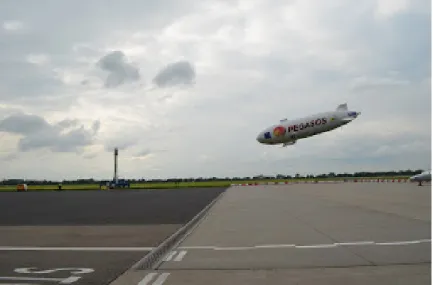
2.1.2 The Zeppelin NT as a measurement platform . . . . 8

2.1.3 Instruments on board . . . . 9

2.2 The model system . . . 10

2.2.1 The meteorological model . . . 11

2.2.2 The chemistry transport model . . . 12

2.2.2.1 Functional principles . . . 12

2.2.2.2 Treatment of aerosols . . . 13

2.2.3 The forecast sequence . . . 14

2.3 Tool developments . . . 17

2.3.1 Online campaign support activities . . . 17

2.3.2 Post campaign developments . . . 17

2.4 Expected challenges . . . 20

2.5 Evaluation metrics . . . 23

3 Description of the data set 25 3.1 Measurement data . . . 25

3.1.1 Observations availability . . . 25

3.2 Model data . . . 27

3.2.1 Grid setup . . . 27

3.2.2 Emissions . . . 27

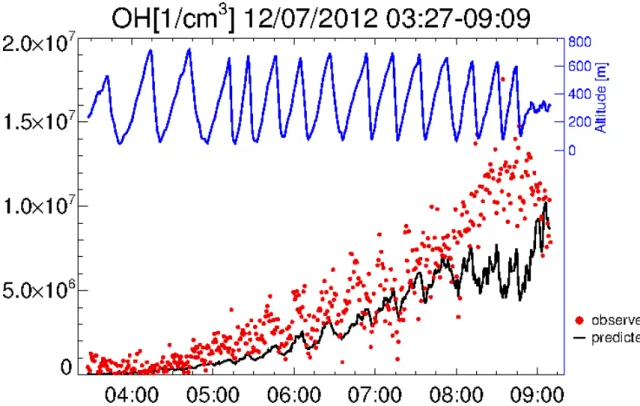
3.3 Illustration of dataset on the example of OH . . . 31

v

vi Contents

4 Results and Discussion 33

4.1 Campaign overall comparison . . . 33

4.1.1 Meteorological parameters . . . 33

4.1.2 Gas phase comparison . . . 40

4.1.3 Aerosol phase comparison . . . 48

4.1.4 Summary . . . 53

4.2 Comparison over height profiling flights . . . 57

4.2.1 Meteorological parameters . . . 57

4.2.2 Gas phase comparison . . . 63

4.2.3 Aerosol phase comparison . . . 71

4.2.4 Summary . . . 77

4.3 Regionality of ammonium-nitrate . . . 81

5 Conclusions 101

A Comparison time-series 105

B Extended metrics table 117

Bibliography 119

Acknowledgements 124

List of Figures

1.1 Effects of aerosols in the atmosphere. . . . . 2 1.2 Idealized planetary boundary layer evolution, adapted by Stull [2012]. . . 3 2.1 The Zeppelin NT airship during landing. . . . . 8 2.2 The scheme of the forward part of the EURAD-IM forecast system. . . . . 16 2.3 Transfer and main measurement area 1km grid boundaries and the Zep-

pelin NT transfer track (red), for the PEGASOS 2012 campains: (A) in the Netherlands, where the CESAR tower is located, and (B) in Italy, where the San Pietro Capofiume site is located. . . . 18 2.4 Snapshot of the Forecast browser. . . . 19 2.5 Time-height plot example with the Zeppelin track overplotted. . . . 20 2.6 Zeppelin track at 2012-07-12 (vertical profiles) plotted with: (A) vertical

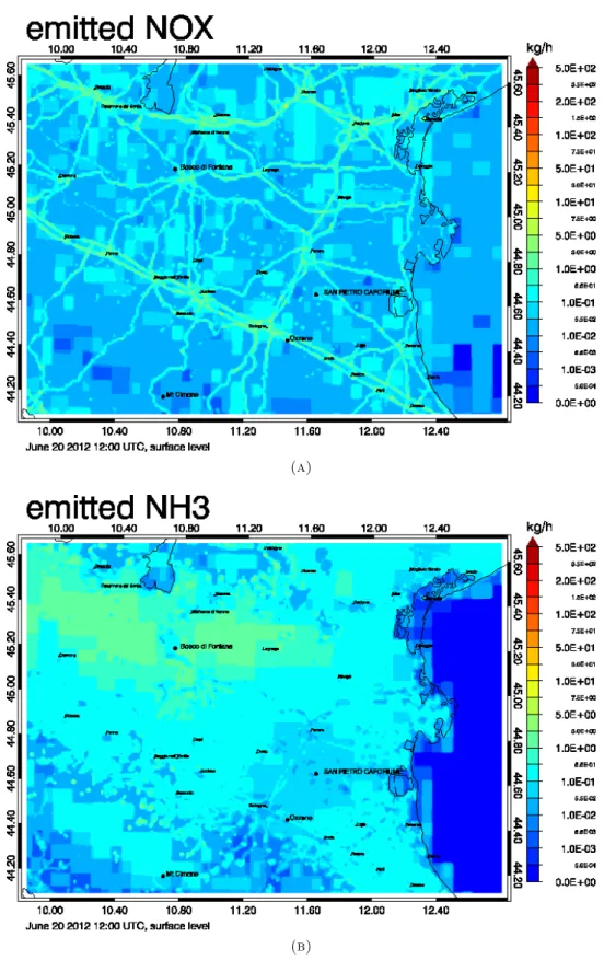
model grid - blue lines and (B) horizontal model grid (cell centers) - blue crosses . . . 22 3.1 Predicted emissions of NOx (A) and NH

(B), for the Cabauw area. . . . 29 3.2 Predicted emissions of NOx (A) and NH

(B), for the Po-Valley area. . . 30 3.3 Example of predicted and observed OH radical along the Zeppelin track. . 31 4.1 Scatterplots of predicted versus observed absolute temperature, for the

Cabauw PEGASOS campaign (A) and the Po-Valley PEGASOS cam- paign (B). Included days are noted in column ’met.’ of Table 3.1. Points are colored with altitude. 1:1 (dashed), 2:1 (dashed-dotted), 10:1 (dotted) lines are indicated. Statistics are shown in Table 4.1. . . . 35 4.2 Scatterplots of predicted versus observed relative humidity, for the Cabauw

PEGASOS campaign (A) and the Po-Valley PEGASOS campaign (B). In- cluded days are noted in column ’met.’ of Table 3.1. Points are colored with altitude. 1:1 (dashed), 2:1 (dashed-dotted), 10:1 (dotted) lines are indicated. Statistics are shown in Table 4.1. . . . 36 4.3 Scatterplots of predicted versus observed water content, for the Cabauw

PEGASOS campaign (A) and the Po-Valley PEGASOS campaign (B).

Included days are noted in column ’met.’ of Table 3.1. Points are colored with altitude. 1:1 (dashed), 2:1 (dashed-dotted), 10:1 (dotted) lines are indicated. Statistics are shown in Table 4.1. . . . 37 4.4 Predicted PBL height (black) for the main measurement days at the lo-

cations of: CESAR tower, Cabauw (19/05/2012-27/05/2012), and San Pietro Capofiume, Po-Valley (18/06/2012-13/07/2012). Lidar retrieved PBL height (violet) at San Pietro Capofiume. . . . 38

vii

viii List of Figures 4.5 Scatterplots of predicted versus observed ozone, for the Cabauw PEGA-

SOS campaign (A) and the Po-Valley PEGASOS campaign (B). Included days are noted in Table 3.1. Points are colored with altitude. 1:1 (dashed), 2:1 (dashed-dotted), 10:1 (dotted) lines are indicated. Statistics are shown in Table 4.1. . . . 41 4.6 Scatterplots of predicted versus observed nitric oxides, for the Cabauw

PEGASOS campaign (A) and the Po-Valley PEGASOS campaign (B).

Included days are noted in Table 3.1. Points are colored with altitude. 1:1 (dashed), 2:1 (dashed-dotted), 10:1 (dotted) lines are indicated. Statistics are shown in Table 4.1. . . . 42 4.7 Scatterplots of predicted versus observed hydroxyl radical, for the Cabauw

PEGASOS campaign (A) and the Po-Valley PEGASOS campaign (B).

Included days are noted in Table 3.1. Points are colored with altitude. 1:1 (dashed), 2:1 (dashed-dotted), 10:1 (dotted) lines are indicated. Statistics are shown in Table 4.1. . . . 43 4.8 Scatterplots of predicted versus observed hydroperoxyl radical, for the

Cabauw PEGASOS campaign (A) and the Po-Valley PEGASOS cam- paign (B). Included days are noted in Table 3.1. Points are colored with altitude. 1:1 (dashed), 2:1 (dashed-dotted), 10:1 (dotted) lines are indi- cated. Statistics are shown in Table 4.1. . . . 44 4.9 Scatterplots of predicted versus observed OH reactivity, for the Cabauw

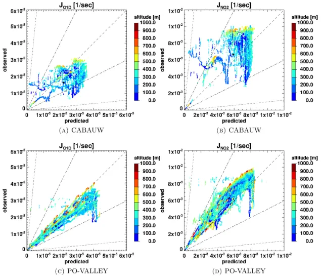
PEGASOS campaign (A) and the Po-Valley PEGASOS campaign (B) re- spectively, colored with altitude. Included days are noted in Table 3.1. 1:1 (dashed), 2:1 (dashed-dotted), 10:1 (dotted) lines are indicated. Statistics are shown in Table 4.1. . . . 46 4.10 Scatterplots of predicted versus observed J

(left) and J

2

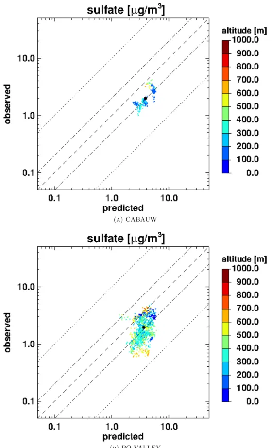
(right), for the Cabauw PEGASOS campaign (top) and the Po-Valley PEGASOS campaign (bottom), colored with altitude. Statistics are shown in Table 4.1. . . . 47 4.11 Scatterplots of predicted versus observed sulfate, for the Cabauw PEGA-

SOS campaign (A) and the Po-Valley PEGASOS campaign (B). Included days are noted in column ’AMS’ of Table 3.1. Points are colored with altitude. Statistics are shown in Table 4.1. Statistics are shown in Table 4.1. . . . 49 4.12 Scatterplots of predicted versus observed ammonium, for the Cabauw

PEGASOS campaign (A) and the Po-Valley PEGASOS campaign (B).

Included days are noted in column ’AMS’ of Table 3.1. Points are colored with altitude. Statistics are shown in Table 4.1. Statistics are shown in Table 4.1. . . . 50 4.13 Scatterplots of predicted versus observed nitrate, for the Cabauw PEGA-

SOS campaign (A) and the Po-Valley PEGASOS campaign (B). Included days are noted in column ’AMS’ of Table 3.1. Points are colored with altitude. Statistics are shown in Table 4.1. Statistics are shown in Table 4.1. . . . 51 4.14 Scatterplots of predicted versus observed organic aerosol, for the Cabauw

PEGASOS campaign (A) and the Po-Valley PEGASOS campaign (B).

Included days are noted in column ’AMS’ of Table 3.1. Points are colored

with altitude. Statistics are shown in Table 4.1. Statistics are shown in

Table 4.1. . . . 52

List of Figures ix 4.15 Mean mass concentrations of predicted and observed aerosols for flights

in Cabauw and Po-Valley. . . . 55 4.16 Scatterplots of temperature, relative humidity and absolute water content,

for the 20/06 (left) and the 12/07 (right), colored by altitude. . . . 58 4.17 Predicted (black) and retrieved only for the 20/06 (violet) PBL height for

the 12/07 and the 20/06 with previous and following days. Airship track (thin black), Monin–Obukhov length (dashed blue). . . . 59 4.18 Virtual potential temperature vertical profiles on 20/06 and 12/07 for

selected time instances: model (black) and observations (red), triangles note the model levels, dashed line notes the predicted PBL height. . . . . 60 4.19 Ground absolute temperature and relative humidity comparison time-

series (left) and scatterplots of the predicted vs observed ground values during the Zeppelin flights F027 (04:36-08:15 UTC) and F028 (08:55-12:04 UTC) (right), at the location of SPC on the 20/06. . . . 62 4.20 Time-height plots of O

, for the San Pietro Capofiume site on: 11/07,

12/07, 13/07, with overlayed observations of 12/07. . . . 65 4.21 Time-height plots of NOx, for the San Pietro Capofiume site on: 11/07,

12/07, 13/07, with overlayed observations of 12/07. . . . 66 4.22 Time-height plots of O

and NOx, for the San Pietro Capofiume site on:

20/06 with overlayed observations. . . . 67 4.23 Scatterplots of O

, NOx, CO, k

, for the 12/07, color-coded with altitude. 68 4.24 Comparison time-series of O

, NOx, CO, k

, along the flight track, for

the 12/07. . . . 69 4.25 k

/NOx characterization plot, for the 12/07 (predicted: black, observed:

red). The shaded area notes regimes of low NOx and high VOC con- centrations, where the non-classical pathway for the OH regeneration is expected to occur, according to Hofzumahaus et al. [2009]. . . . 69 4.26 Time-height plots of sulfate, for the San Pietro Capofiume site on: 19/06,

20/06, 21/06, with overlayed observations of 20/06. . . . 73 4.27 Time-height plots of ammonium, for the San Pietro Capofiume site on:

19/06, 20/06, 21/06, with overlayed observations of 20/06. . . . 74 4.28 Time-height plots of nitrate, for the San Pietro Capofiume site on: 19/06,

20/06, 21/06, with overlayed observations of 20/06. . . . 75 4.29 Scatterplots of sulfate, ammonium, nitrate, organics, for the 20/06, color-

coded with altitude. . . . 76 4.30 Comparison time-series of nitrate, ammonium, temperature, relative hu-

midity, along the flight track, for the 20/06. . . . 77 4.31 Scatterplot of predicted versus observed nitrate (SPC on 20/06/2012),

colored with: (A) temperature discrepancy ∆T, (B) relative humidity dis- crepancy ∆RH, where ∆X= X

-X

, 1:1(dashed), 2:1(dashed- dotted),10:1 (dotted). . . . 78 4.32 Display of observed aerosol mass concentrations of sulfate (red), nitrate

(blue), and organics (green), versus the time the sampled air (coming from the Apennines) had spend in the Po-Valley according to 24h backward trajectories for the 21/06/2012. Figure adopted from Rubach [2013]. . . . 82 4.33 Zeppelin track on 20/06 (near SPC at Po-Valley): (top) Zeppelin altitude

versus time, bined by altitude (bins:0-200 m, 200-600 m, 600-800 m). The

solid thick line represents the predicted PBL height, (bottom) Zeppelin

track on latitude/longitude projection with grid cell centers as blue crosses. 83

x List of Figures 4.34 Scatterplots of sulfate, ammonium, nitrate, on 20/06, bined by flight al-

titude as illustrated in Figure 4.33. The top row panels dispay the full dataset for that day. The following three row panels display the subsets for the same day for the altitude spans 0-200 m, 200-600 m, and 600-800

m, from bottom to top, respectively. Statistics are noted in Table 4.4. . . 84

4.35 Scatterplots of sulfate, ammonium, nitrate, on 20/06, color-coded with time, separating the flight by mixing conditions: from 04:00 to 09:00 the PBL is under development, from 09:00 to 13:00 the PBL is fully developed. Statistics are noted in Table 4.4. . . . 85

4.36 Predicted versus observed neutrality, as mass concentration of ammonium in excess to anionic components sulfate and nitrate, on 20/06. . . . 86

4.37 Left column: Time-series of predicted gas-phase H

SO

, NH

, HNO

con- centrations along the flight track (left axis), with overplotted the SO

, NH

, NO

surface emissions directly below (right axis). Right column: Predicted and observed concentrations of the corresponding aerosol com- ponents sulfate, ammonium, nitrate (left axis), with overplotted the pre- dicted production rates of H

SO

, HNO

, and the altitude, along the flight track (right axis). The production rates correspond to the reac- tions OH + SO

− − → HSO

(rate limiting for the production of H

SO

) and OH + NO

− − → HNO

. . . . 89

4.38 Predicted production rates of H

SO

and HNO

corresponding to the oxidation reactions of SO

and NO

, at the ground level, at 06:00 UTC, over the Po-Valley. . . . 90

4.39 Predicted and observed wind velocity, along the flight track on the 20/06. 93 4.40 Distribution of predicted sulfate (left), ammonium (middle), and nitrate (right) concentration at 06:00 UTC 06/2012, at the 5th (bottom) and 9th (top) model layers with altitude extensions (at the location of SPC) 161-243m and 578-749m respectively. . . . 94

4.41 Top: Concentration of the ’on site’ formed precursors H

SO

and HNO

, estimated from the predicted production rates r

and r

. Bottom: Sum of gas precursor concentration and respective particle concentration (H

SO

(g)+sulfate, NH

(g)+ammonium, HNO

(g)+nitrate), along the flight track on the 20/06. . . . 96

A.1 Comparison timeseries - observed(red), predicted(black): temperature. . . 106

A.2 Comparison timeseries - observed(red), predicted(black): rel.humidity. . . 107

A.3 Comparison timeseries - observed(red), predicted(black): O

. . . . 108

A.4 Comparison timeseries - observed(red), predicted(black): NO

. . . . 109

A.5 Comparison timeseries - observed(red), predicted(black): OH. . . . 110

A.6 Comparison timeseries - observed(red), predicted(black): HO

. . . . 111

A.7 Comparison timeseries - observed(red), predicted(black): k

. . . . 112

A.8 Comparison timeseries - observed(red), predicted(black): sulfate. . . . 113

A.9 Comparison timeseries - observed(red), predicted(black): ammonium. . . 114

A.10 Comparison timeseries - observed(red), predicted(black): nitrate. . . . 115

List of Tables

2.1 Aerosol species processed in MADE and their modal assignment. . . . 14 3.1 Observations availability for the two 2012 PEGASOS campaigns. The

column ’met.’ stand for the meteorological variables, and the column AMS stands for the Aerosol Mass Spectometer measurements. . . . 26 3.2 Parameters of the coarse (15 km), fine (5 km), and finest (1 km) compu-

tational domains. . . . 27 4.1 Statistic parameters for the two 2012 PEGASOS campaigns: Cabauw,

Netherlands and Po-Valley, Italy. Included days are noted in Table 3.1. . 56 4.2 Statistic parameters calculated for two measurement days in Po-Valley:

12 July 2012 (top), 20 June 2012 (bottom). . . . 80 4.3 Correlation coefficients for the pairs sulfate-r

and nitrate-r

cal-

culated for the flight of 20/06 and separately for the two parts of the flight. . . . 93 4.4 Statistic parameters calculated for the 20 June 2012, by altitude, and by

mixing conditions. . . . 99 B.1 Extended statistic parameter table, for the two 2012 PEGASOS cam-

paigns. Included days are noted in Table 3.1. . . . 118

xi

Chapter 1

Introduction

The lowest layer of the atmosphere, and the most important for life on Earth, is called the troposphere. Its importance lies on two facts. On one hand, within the troposphere almost everything classified as weather takes place, which has an impact on the human activities. On the other, whatever composes the tropospheric air is what all the living creatures breathe.

The troposphere ranges in thickness from 8 km at the poles to 16 km over the equator and is bounded above by the tropopause. The vertical profiles of pressure and density are approximated by considering the atmosphere in an hydrostatic equilibrium. The hydrostatic law that results, causes air pressure and density to decrease approximately exponentially with increasing altitude, as described in Bohren and Albrecht [1998], so that the largest fraction of the total atmospheric mass (the latter being 5.14 ×10

kg, as determined by Trenberth and Guillemot [1994]), is located in the troposphere. Below the tropopause, the altitude of which depends on latitude and season, temperature increases strongly moving down through the troposphere, to the surface.

Throughout most of the atmosphere, the air acts as a carrier for a large number of trace gases and a mixture of solid and liquid materials in the form of finely dispersed particles.

These assemblies of particles suspended in the air are called aerosols. In atmospheric science, aerosols are defined as minute particles suspended in the atmosphere. Their presence is noticed directly, as they scatter and absorb sunlight. Their scattering of sunlight gives the red-yellow colors in sunrises and sunsets, and reduces visibility (Figure 1.1). This visibility, is determined by the mass and size distribution of aerosols in the air (Lee et al. [2005]). While, the horizontal visibility is important for the road traffic, the vertical visibility plays a significant role as well, especially in aviation and astronomy. As an indirect effect, aerosols in the lower atmosphere can modify the size of cloud particles,

1

2 Chapter 1. Introduction

Figure 1.1: Effects of aerosols in the atmosphere.

changing how the clouds reflect and absorb sunlight, thereby affecting the Earth’s energy budget (Ball and Robinson [1982]).

Aerosols are divided in two categories according to their origin: primary and secondary.

Primary aerosols are those directly emitted and appear in the atmosphere as already shaped particles. They result from fragmentation processes in the Earth’s surface, or from high temperature processes. Secondary aerosol particles appear in the atmosphere from “nothing” as a result of gas-to-particle conversion. Because of that, these secondary aerosols are present in the sub-micron size fraction. This process, is accomplished either by condensation, which adds mass onto pre-existing aerosols, or by direct nucleation from gaseous precursors.

As far as inorganic secondary aerosol formation is conserned, ammonia (NH

), a predom- inant alkaline component in the atmosphere, reacts with acid gases and forms ammo- nium (NH

) aerosol salts. Sulfuric acid (H

SO

), as the product of the sulfur dioxide (SO

) oxidation, is the main gaseous precursor for sulfate aerosol. Its reaction with NH

forms ammonium-bisulfate ((NH

)HSO

) and subsequently ammonium-sulphate ((NH

)

SO

). Nitric acid (HNO

), as the product of nitrogen dioxide (NO

) reaction with hydroxyl radicals (OH) during the day, or as the product of dinitrogen pentoxide (N

O

) reaction with water during the night is the main gaseous precursor for nitrate aerosols (NO

). The reaction of HNO

with NH

forms ammonium-nitrate (NH

NO

).

The partioning between gas (g) and aerosol (s) phase for sulfate and nitrate is described by the reactions 1.1 and 1.2.

H

SO

(g) + NH

(g) −− ) −− * (NH

)HSO

(s) (1.1) HNO

(g) + NH

(g) −− ) −− * (NH

)NO

(s) (1.2)

Organics, in gaseous form, are also present in the atmosphere. Volatile organic com-

pounds (VOCs), are emitted from plants and trees (like isoprene, monoterpenes and

sesquiterpenes), but also from vehicles and industry (aromatics), or other airborne ac-

tivities. When entering the atmosphere, oxidation of VOCs from hydroxyl (OH), O

,

Chapter 1. Introduction 3

Figure 1.2: Idealized planetary boundary layer evolution, adapted by Stull [2012].

or HNO

, takes place (Griffin et al. [1999]). The oxidation products, are less volatile than the reactants. When the supersaturation of a product is high enough to overcome the nucleation barrier given by the Kelvin effect, it will condense and form particles.

This process is called homogeneous nucleation. When pre-existing aerosols are available, the oxidation products can condense on these without supersaturation, if the saturation vapour pressure, determined by the mixture is reached. Secondary organic aerosols, since they have a large number of different components, are in general difficult to be studied.

As a result of these mechanisms, the composition of aerosols in a local area is largely influenced by the concentrations of NH

, H

SO

, HNO

, organics, and water vapour in the atmosphere. The chemical transformations that occur in the troposphere, so between different gas compounds, as between gas and aerosol compounds, are more prominent and important in the planetary boundary layer (PBL).

The PBL is defined as the lowest part of the atmosphere, in contact with the planetary

surface. The thickness of the PBL is variable and evolves as a function of daytime, as

shown in Figure 1.2, since the heat transfer from the surface depends on the diurnal

heating of the surface from the sun. In the morning, the earth’s surface is warmed up by

solar radiation so the lower layers are heated up, while cooler layers lie above, leading

to the development (rise) of a convectively mixed layer (ML). In the evening, radiative

heating from the ground is absent. The temperatures of layers closer to the ground are

lowered, while still warmer air lies in higher layers, above. The mixing with air parcels

from above is prevented and a stable layer is formed at the earth’s surface, called stable

nocturnal boundary layer (NBL). Because the NBL develops from the ground, the air

above it separates the ML from the ground and preserves the properties of the previous

4 Chapter 1. Introduction day’s ML, without direct contact to the surface. Reflecting the residual of the previous day’s ML, the layer above the NBL is defined as the residual layer (RL). In the next morning, radiative heating starts again and a new ML develops by attenuating first the NBL and then the RL. The thin layer where stable air from above enters (entrains) the convective ML is defined as the entrainment zone. In order to study the diurnal evolution of the PBL and its effect on the chemical constituent concentrations, it appears necessary to perform measurements, on one hand with a time extend from the early morning hours to noon, and on the other, with a vertical extend from the surface up to an altitude comparable with the maximum PBL height.

During the most of the previous field campaigns, the observations that have been used were ground based. Those include measurements at stable points in space which are usually in the low surface layer, whether studying gas phase (Rohrer et al. [1998], Han et al. [2011]), or aerosol phase (Spracklen et al. [2011], Crippa et al. [2014], Aan de Brugh et al. [2012]). The variability in the concentrations close to the surface due to an evolving PBL has been captured, but little information can be derived about the variability in the higher altitudes. Airborne studies have also been done in the past (Shon et al. [2008], Menut et al. [2000], Reddington et al. [2011]), where fast moving aircrafts have been used. However, those aircrafts were not proven to be suitable for the study of processes in the PBL for the following reasons. First, the aircraft velocity was relatively high as compared to the slow PBL evolution. Second, the distance covered in only some minutes was long to study the local PBL evolution. Finally, the high flight altitude was too high as compared with the PBL height. Using the Zeppelin NT as a platform of gas and aerosol measurement instruments in the PBL, overcomes the above limitations. The ability to perform flights at low velocities in altitudes lower than 1000 m above the surface, makes it the ideal platform for characterizing the processes within the PBL.

In addition, nitrate, as an aerosol component, has received comparatively little attention.

It is not as easily predicted as sulfate, since it is partly transported and partly locally produced, making the distinction between the ’transported’ component and the ’local’

component not straightforward. However, in studies including nitrate, it is shown that it is an important aerosol species both today and over the 21st Century and important in areas where large urban and agricultural emissions coincide (Walker et al. [2012]).

In addition, as noted in Schmidt et al. [2014], nitrate was only included in two of the models that contributed to the Coupled Model Intercomparison Project (CMIP5) and this inclusion brought models closer to the observed surface temperature trend.

Linking the above, it is apparent that the dataset compiled by on board the Zeppelin

NT observations, is unique and promising. It can provide a new insight to processes in

Chapter 1. Introduction 5 terms of high resolution vertical profiles, dynamics, and chemistry, both gas and aerosol phase.

A significant part of this work was focused on the set up of an operational forecast system running on a 1 km spatial resolution grid as a means of online support during the course of a measurement campaign. This included the meteorological initialization on a 1 km gridded topology, allowing consequently the extension of the chemistry transport model to a 1 km horizontal resolution, by using aggregated emission fields in the same resolution.

The main target of this work was to enable the comparison of the measurements by instruments on board on the Zeppelin NT with the output of a regional chemistry trans- port model. Chemical constituents treated, include both gas-phase and aerosol species.

The model is evaluated over the course of a seven week period, covering two campaigns in 2012, in two European countries. A better understanding of the success and/or fail- ure of the model to capture observations is aimed by studying specific campaign days.

Finally, a discussion aims to investigate the regional character of sulfate, ammonium,

and nitrate aerosol components.

Chapter 2

Methodology

2.1 The PEGASOS project

2.1.1 Project description

The Pan-European Gas-AeroSOls-climate interaction Study (PEGASOS), as a European large scale integrating project, had the target to study in which degree do the regional atmospheric processes affect global processes and vice versa, as concerns both chemistry and changing climate. The ultimate aim is the reduction of the uncertainty of those feedbacks. In addition, mitigation strategies and policies will be proposed, in order to improve air quality while limiting their impact on climate change. In order to optimize the methodologies and the understanding of air quality and climate interactions, the project was organized into separate scientific themes. The first theme was the anthro- pogenic and biogenic emissions and their response to climate and socio-economy. The second theme was the atmospheric interactions among chemical and physical processes.

The third theme was the regional and global links between atmospheric chemistry and climate change. Finally, the last theme was the air quality in a changing climate and the integration with policy.

Local pollutant exchanges from surface to air and vice versa, air quality, and weather are undoubtedly connected with global atmospheric chemistry and climate. However, the aforementioned operate in different temporal and spatial scales. The PEGASOS project aims to provide understanding about the connection between those scales by studying the area of Europe considering changing pollutant emissions with a time horizon of 50 years. In order to quantify the feedbacks between air quality and a changing climate our understanding of several atmospheric processes needs to be improved. Within the project, the dynamically changing emissions and deposition will be analysed and linked

7

8 Chapter 2. Methodology

Figure 2.1: The Zeppelin NT airship during landing.

to tropospheric chemical reactions and interactions with climate. The emerging con- nections between chemistry-climate and surface processes will be presented. Scales of study include local, regional and global phenomena. Because of the complexity of the processes under study the need of a unique measurement platform, the Zeppelin NT, has risen.

In 2012 and 2013, airship based measurements of gas phase and aerosol phase were performed in several European regions. The Zeppelin NT, equipped with measurement instruments, was transferred to the Cabauw region in the Netherlands, from 19 May to 27 May 2012, to the Po-Valley region in Northern italy, from 18 June to 13 July 2012, and the following year, 2013, to the Hyyti¨ al¨ a and J¨ amij¨ arvi regions in Finland.

2.1.2 The Zeppelin NT as a measurement platform

The Zeppelin NT is a semi-rigid airship that has a total length of 75 m and a maximum hull diameter of 14m (Figure 2.1). Its skeletal carbon structure is covered by multilayer laminate. The hull is inflated with helium (He) which is used as a lifting gas. Together with the attached propellers, the Zeppelin NT achieves the required uplift with a maxi- mum payload of 1900 kg. The three propeller configuration (one at the back and two at the sides) allows for take-off and landing without horizontal velocity. Depending on the weather conditions, the Zeppelin NT has a maximum flight endurance of 24 h. It has a maximum cruising speed of 115 km/h, a maximum range of 900 km, and a maximum flight altitude of 2600 m.

However, the actual maximum altitude is limited by the following factors. First, the

expansion of He in the hull, because of reduced outside pressure when in altitude, has

Chapter 2. Methodology 9 a limit for the sake of the Zeppelin integrity, setting a pressure limit. While altitude increases, the He expansion is assisted by Ballonets (additions inside the hull inflated with ambient air), which at the same time lose air. At the point where the maximum pressure of He has been reached and the Ballonets have lost all their air, the maximum altitude has been reached. However, the heavier the payload, more He has to be inflated in the hull, allowing less inflated Ballonets at ground level which consequently limits the allowable He expansion. Second, when the ambient temperature increases, the ambient air density decreases, so the difference in density between ambient air and He decreases and so does the lifting capacity. Opposing, when the temperature of the hull increases due to solar radiation, the He density decreases, so the difference in density between ambient air and He increases (superheat effect) and so does the lifting capacity. Taking into account all the above, with full scientific payload, the maximum altitude, during the campaign, varied between 400 m and 750 m.

2.1.3 Instruments on board

For the PEGASOS campaigns a variety of instruments were developed and adapted to fulfil the Zeppelin requirements. These requirements include the minimum possible weight, so that altitude and flight endurance are affected as little as possible, and the mounting onto fixed points, in agreement with airship security regulations. Light racks, mountable to the seat rail inside the Zeppelin cabin, were developed for the purpose of hosting the electronics and parts of the instruments. However, space and payload limita- tions did not allow simultaneous installation of all. Three combinations of instruments, named cabin layouts (CL), were decided in advance in such a way that each combination corresponded to a different scientific task.

Several instrument racks were present in every cabin layout. These were the COD, CPN, NOX and Top-Platform. The COD instrument measured the CO concentration. The CPN rack included instruments to measure particle size distribution and particle number concentration. The NOX rack included instruments measuring concentrations of NO, NO

, and O

and upwelling spectral actinic flux. Photolysis frequencies were calculated from the upwelling and the downwelling spectral flux measured at the Top-Platform.

In the Top-Platform instruments that measured the concentrations of the radicals OH and HO

as well as the total OH reactivity. The always present instrument group is completed with the addition of the meteorological boom which measured temperature, relative humidity, and three dimensional wind.

The cabin layout CL8 aimed to a detailed photochemistry characterization. In addition

to the always present instruments it contained the LOP, FFL, and HGC racks. The

10 Chapter 2. Methodology LOP rack contained an instrument detecting HONO. The FFL rack contained an in- strument measuring HCHO. The HGC rack included instruments that determined VOC concentrations.

The cabin layout CL9 was compiled in order to investigate the process of nucleation.

Together with the always present, the API and the NAS were added. The first one can determine the composition of naturally charged ions and clusters while the second one measures the distribution of ions over a range of electrical mobilities, and the distribution of particles between 2nm and 40nm.

Finally, the cabin layout CL5 was used to study secondary organic aerosols (SOA).

The PSI rack and the AMS instrument, were added to the constant configuration. The PSI included instruments that measured black carbon mass concentration, number size distribution of particles with diameters larger than 200nm as well as hygroscopicity (a factor that characterizes particle growth). The AMS instrument is described in the following paragraph.

The development and installation of the AMS instrument under the Zeppelin require- ments is described in detail in Rubach [2013]. The particles are sampled through an inlet followed by an aerodynamic lens that focuses particles with size between 0.1 µm and 0.7 µm on a beam. Entering a vacuum chamber, particles are accelerated to velocities inverse proportional to their size, before entering the particle sizing chamber, in which packages of particles are created with common starting point and starting time (by a chopper) but different velocities. They are directed into the particle detection chamber where they are impacted on a heated surface and vaporized. The resulting ions then are accelerated by electrostatic fields into a mass spectrometer which detects ion rates on a mass to charge ratios spectrum. These ion rates are interpreted as mass concentrations of the different aerosol species.

2.2 The model system

The EURAD-IM (EURopean Air pollution and Dispersion) model system is a numer-

ical model system able to simulate the physical and chemical evolution of trace gases

and aerosols in the troposphere and lower stratosphere. The suffix IM (Inverse Model)

indicates that the system has been expanded by an inverse part. The forward part of

the model system - the standard forecast system that is used in this work - consists of

two major models: First, the meteorological model WRF (Weather Research and Fore-

cast) acts as the meteorological driver for the chemistry transport model. It calculates

Chapter 2. Methodology 11 and delivers the meteorological fields that are necessary like wind, temperature and rel- ative humidity. Second, the EURAD-IM chemistry transport model (EURAD-CTM) is a mesoscale model that simulates the processes of horizontal and vertical diffusion, horizontal and vertical advection, chemical transformation, and wet/dry deposition, for tropospheric gases and aerosols.

2.2.1 The meteorological model

The WRF model is a numerical weather prediction model designed for both research and operational applications. The non-hydrostatic fully compressible Euler equations are solved to calculate the prognostic variables:

• horizontal velocity components u and v (in Cartesian coordinate),

• vertical velocity w,

• perturbation potential temperature,

• perturbation geopotential,

• perturbation surface pressure of dry air,

• and a number of optional variables as turbulent kinetic energy and water vapor mixing ratio.

The horizontal grid follows the Arakawa C-grid staggering. The vertical grid follows the terrain (sigma levels), with vertical stretching permitted, so the vertical levels are defined as:

σ

= p

− p

p

− p

(2.1) where:

• k the layer number

• p

the pressure at layer k

• p

the pressure at the surface

• p

the pressure at the top of the model domain, which is kept constant (1000 Hp)

The time integration is done using a 2nd- or 3rd- order Runge-Kutta scheme with vari-

able time step capability.

12 Chapter 2. Methodology 2.2.2 The chemistry transport model

2.2.2.1 Functional principles

The EURAD-IM chemical transport model (CTM) is an Eulerian meso-scale model involving advection, diffusion, chemical transformation, wet and dry deposition and sed- imentation of tropospheric trace gases and aerosols (Jakobs et al. [1995],Memmesheimer et al. [2004]). It solves the following equation:

∂c

∂t = −∇(uc

) + ∇(K∇c

) + E

+ F

+ ∂c

∂t |

+ ∂c

∂t |

+ ∂c

∂t |

(2.2) and with c

indicating the mean concentration of the species i, the terms on the right hand side of the Equation 2.2 represent changes of concentration due to the following processes:

• ∇(uc

): advection meaning transport by wind, where u is the wind velocity vector

• ∇(K∇c

): turbulent diffusion

• E

: emission rates

• F

: fluxes

•

|

: gas phase chemical conversion

•

|

: transport in clouds, aqueous chemistry and wet deposition

•

|

: aerosol chemistry (processed in MADE)

The operator splitting technique is applied in a way that advection and diffusion are applied symmetrically around the solver modules for gas and aerosol phase processes.

The model state is updated in time as follows:

x

(t + ∆t) = T

T

D

CM D

T

T

x

(t) (2.3) where:

• x

(t + ∆t) the model state, that is concentration/mixing ratio of species i

• t the time step

• ∆t the length of a time step

• T

the advection module in horizontal direction

Chapter 2. Methodology 13

• T

the advection module in vertical direction

• D

the vertical diffusion

• C the gas-phase chemistry solver

• M the aerosol dynamics solver

The T and D operators are applied at one half of the model’s timestep before and one half after the C and M operators.

2.2.2.2 Treatment of aerosols

Within the CTM, aerosols are treated by the Modal Aerosol Dynamics module for Europe (MADE). Based on gas-phase concentrations calculated during the CTM run, meteorological values provided by the WRF, and emissions, the MADE simulates the bidirectional transfer between gas and aerosol phase, in a way that aerosol and gas phase are directly coupled.

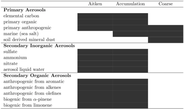
As concerns size, MADE is trimodal, that is, the particles are separated into three modes.

The coarse particles, making the coarse mode, namely marine sea salt, mineral dust, and coarse particles of anthropogenic origin, are primary aerosols with no exception, meaning they are emitted as they are. The minimum median diameter of this mode is 1.0 µm. The fine particles are separated into two modes. The Aitken mode, representing freshly emerged, very small aerosols, has a minimum median diameter of 0.01 µm. The accumulation mode, representing aged aerosols, has a minimum median diameter of 0.07 µm. Particles in the Aitken mode have high number concentration, especially near their source, and through the process of coagulation (the collision of two particles into one), end up relatively fast in the accumulation mode. However, particles in the accumulation mode coagulate slowly to reach the coarse mode. Sulfate, ammonium, nitrate and organics masses are assigned to the fine particle category, with median diameter less than 1.0 µm but with most of the mass in less than 0.75 µm. So the modeled sum of Aitken and Accumulation mode for the three prementioned aerosol species is comparable to the AMS measurements. Table 2.1, lists aerosol species treated in MADE with their modal assignment.

For fine particles, the most important mechanism is the solution of the equilibrium of the

system H

—NH

—SO

—NO

—H

O. The solution, based on the Pitzer-Simonson-

Clegg model from Clegg et al. [1992] and the Analytical Predictor for Condensation

described in Jacobson [1997], namely PSC/APC, is implemented and developed using

an iterative approach with temperature dependant activity coefficients (factor used in

14 Chapter 2. Methodology Aitken Accumulation Coarse Primary Aerosols

elemental carbon primary organic primary anthropogenic marine (sea salt)

soil derived mineral dust

Secondary Inorganic Aerosols sulfate

ammonium nitrate

aerosol liquid water

Secondary Organic Aerosols anthropogenic from aromatic anthropogenic from alkenes anthropogenic from olefines biogenic from α-pinene biogenic from limonene

Table 2.1: Aerosol species processed in MADE and their modal assignment.

thermodynamics to account for deviations from ideal behaviour), by Friese and Ebel [2010]. Even though this solution is accurate, it is also computationally demanding due to its iterative nature. For operational purposes, a High Dimensional Model Rep- resentation (HDMR) from PSC/APC was built and implemented by Nieradzik [2005], which significantly reduces computing time and allows for three dimensional chemistry transport calculations.

2.2.3 The forecast sequence

The daily chemical weather forecast that was used in this project is shown in Figure 2.2, and the following description refers to the same figure. First, the meteorology part is initiated (light blue). After the area of interest has been chosen and projected in the model domain the terrestrial data is downloaded, which includes topography information like surface height above sea level as well as soil type and vegetation. This data, in addition to meteorological initial (meteorological state at 24:00 UTC of previous day) and boundary (meteorological state at line enclosing area of interest, taken from a global meteorological model) is needed for the meteorology calculation of the ’current’

day of interest. This calculation, as described in 2.2.1 provides the meteorological fields

of the projected area. Secondly, as a preparation for the chemistry transport model

the emissions fields should be processed to fit the area of interest and the ’current’

Chapter 2. Methodology 15 day (yellow). The TNO 2012 emission inventories are used as a primary source. From these inventories the area of interest is cut to fit our area of interest and the model resolution. This process includes the calculation of the hourly emission rates from the yearly rates taking into account the day of year, meteorology as well as mean human hourly activity. In addition, since a comparison with the Zeppelin observations is desired, the raw observations data is processed, so that each measurement is given a time/location in the model timeframe/domain (red).

The above mentioned, together with chemical initial (chemical state at 24:00 UTC of

previous day, taken from the previous day chemical forecast) and boundary (chemical

state at line enclosing area of interest, taken from a global model for the coarse grid or

from the mother domain for a nest grid) conditions, make the input for the chemical

transport model. This calculation provides the chemistry fields, for gas and aerosol

phase for the the initially chosen area, as well as the one to one (measurement-model

value) comparison.

16 Chapter 2. Methodology

Figure 2.2: The sc heme of the forw ard part of the EURAD-IM forecast system.

Chapter 2. Methodology 17

2.3 Tool developments

2.3.1 Online campaign support activities

As part of support activities, a special chemical and meteorological forecast tool for flight missions has been developed. Operated at the Rhenish Institute of Environmental Research at the University of Cologne (RIU), the EURAD-IM model has been extended to versatile high resolution (1km) model domains for operational mission planning. This system was operated on a dedicated computing platform, which allows for daily forecasts with fixed schedule, and was applied to both PEGASOS campaigns of spring 2012 and spring 2013.

Within the operational forecast chain two fixed grids are being computed for the areas of greater Europe (p15, with a resolution of 15km) and Central Europe (p05, 5km). During a campaign, the measurement area and consequently the calculation area can change by day. To account for this, a sequence of ”jumping” grids (jc1, with a resolution of 1km) was set up, covering both the transfer flights from the airport of Friedrichshafen to the main measurement areas, and the daily flight patterns (transects or vertical profiles). In addition, an alternative or ”follow-up” grid has been simulated to provide a forecast for the most probable (next day) region to succeed the current location of the Zeppelin NT.

In order to operate the jumping grids, the input files of EURAD-IM should be prepared or ”cut” beforehand to the respective grid parameters and that is meteorology - which is provided by the WRF model, and emissions which are cut beforehand by a ”mother”

emission grid (GIS aggregated TNO data) to meet the position and size of the 1km grid.

The 1km grids, as support to the PEGASOS 2012 campaigns to the Netherlands and to northern Italy, together with the Zeppelin transfer track are shown in 2.3.

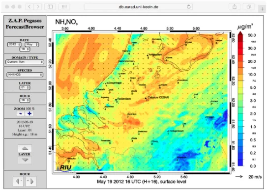
The forecast results have been presented on an online ”forecast browser” (e.g. for the PEGASOS campaign: http://www.riu.uni-koeln.de/PEGASOS/) for selected species at a selected number of model layers. The ”forecast browser” (that is an online image- viewer), has been created to provide an easy-to-use tool to browse the forecast products in time, height, species, and domain. Different types of visualizations were available like horizontal 2d plots, time-height plots, vertical cross-sections and time-series. A snapshot of the ”forecast browser” displaying a horizontal 2d plot is shown in Figure 2.4.

2.3.2 Post campaign developments

After the campaigns, and when the measurement data was made available, additional

processing was done to enable the measurement-model comparison and interpretation.

18 Chapter 2. Methodology

(a)

(b)

Figure 2.3: Transfer and main measurement area 1km grid boundaries and the Zep-

pelin NT transfer track (red), for the PEGASOS 2012 campains: (A) in the Netherlands,

where the CESAR tower is located, and (B) in Italy, where the San Pietro Capofiume

site is located.

Chapter 2. Methodology 19

Figure 2.4: Snapshot of the Forecast browser.

First, in the pre-processor of EURAD-IM for observations, a part was added to account for the PEGASOS observations for all the measured species and parameters. By mapping the Zeppelin track in the three-dimensional model domain at the correct time, each observed value corresponds to a predicted value.

In addition, since the study was focused on vertical profiles, a type of time-height plot

(Hovm¨ oller) was developed, that displays the diurnal vertical profile evolution. During

the model calculation, which has a time resolution with respect to the horizontal resolu-

tion of the configured grid (60-300 sec), the concentrations and parameters are updated

for output with a time resolution of 10 min (higher than the default output time res-

olution of 1 h), for the Zeppelin location, for all the model levels (from the surface to

a selected maximum height). For this location then, the vertical profile is color coded

and plotted from 00:00 to 24:00 as a background. Then the measurements along the

Zeppelin track can be overlayed with the same color coding to enable comparison. An

example for predicted O

on 2012-07-12 together with the Zeppelin track at that day, is

shown in Figure 2.5.

20 Chapter 2. Methodology

Figure 2.5: Time-height plot example with the Zeppelin track overplotted.

2.4 Expected challenges

The aim of this thesis is to compare results from a regional model with observations along the Zeppelin NT track. Expected difficulties that are related to the spatial and temporal resolution of the model as compared with the Zeppelin track and time resolution of measurements are mentioned as follows:

First, the comparison is done ’point to point’, without taking mean values. Each mea- surement is compared with the respective value in the model, without interpolation.

Taking this into account, it is known from the beginning that the observations will not be captured in detail. Even though the general dynamics and chemistry features will appear in the model, that doesnt mean that they will appear in the exact same time and location as in the measurements.

Second, unlike ground measurements that are able to measure through 24 hours of a day, the Zeppelin NT has a short measuring time span. So, instead of studying the diurnal evolution for constituents, which would have been easier as concerns the comparison with a model, observations span only several hours (the vertical profile with the longest duration is about 6 hours on 2012-07-12). It would have been interesting to have measurement time frames that start in the evening and finish in the morning of the next day. Since these kind of flights were not performed, there are no observations during the evening breaking up of the PBL, and this process will not be treated in this thesis.

The horizontal resolution of the model is 1 km. However, the Zeppelin perfomed vertical profiles by circling a location with a radius of about 500 meters as shown in Figure 2.6.

As a result, the horizontal movement could span maximum 4 grid boxes in the model

Chapter 2. Methodology 21 domain. That could give unwanted, but explained concentration fluctuations due to the space discretization. The vertical resolution of the model is variable with height with denser levels close to the surface. The vertical profiles were performed with a maximum height of 800-1000 meters which spans 7 to 9 layers in the model domain.

For one ascending of the Zeppelin only 7-9 model points are given for comparison. As an example, for the vertical profile at 4:00 of 2012-07-12, shown in Figure 2.6, the measurements can be compared with 8 model values. In the diurnal boundary layer cycle the dynamics that occur are expected to be somewhat resolved but in a coarse way in comparison with the measurement resolution.

In general, the exact mixed layer height is difficult to be predicted as it is difficult to have a very good representation of the meteorological and dynamical conditions. Studies have shown (as an example Viterbo et al. [1999]) that even with the same forcing conditions but with (slightly) different stability treatment in the mixing scheme, big differences in the mixed layer height are produced. The prediction efficiency depends on how much of the micrometeorology is captured by the model as well as how exact are the calculated values for the heat, latent and sensible (latent is related to changes in phase between liquids, gases, and solids while sensible is related to changes in temperature with no change in phase), and relative humidity. The knowledge of the correct soil heat capacity also plays a sygnificant role as it determines the soil response to heating from the sun.

Today, the mixed layer height can be predicted within an uncertainty of approximately

100 meters. Since the mixing conditions are those who determine the vertical transport

of chemical constituents, it is known from the beginning that differences between the

predicted and observed mixed layer height will have undoubtely an big effect on the

prediction quality of all chemical species.

22 Chapter 2. Methodology

(a)

(b)

Figure 2.6: Zeppelin track at 2012-07-12 (vertical profiles) plotted with: (A) vertical

model grid - blue lines and (B) horizontal model grid (cell centers) - blue crosses

Chapter 2. Methodology 23

2.5 Evaluation metrics

In order to evaluate a model against observations, one can select among a variety of statistical metrics. The large number and the diversity of the existing metrics makes the selection for the judjement of the overall model performance difficult. In addition, several of these metrics are not efficient, since they are subject to assymetry and/or bias. In this project, as a first measure of the model performance, the mean value of observations ( ¯ O), and the mean value of respective predictions ( ¯ M ) is calculated. These mean values are combined graphically yielding the center of gravity (COG) in a scatterplot where all observations are plotted in the y axis and the respective predictions in the x axis. In this case, the center of gravity has coordinates:

[cog

, cog

] = [ ¯ M , O] ¯ (2.4) A new set of metrics is proposed in Yu et al. [2006], based on the concept of factors, that is both unbiased and symmetric. This means, first that the undue influence of small numbers in denominator is avoided, and second that overprediction and underprediction are treated proportionately. In this project, the normalized mean bias factor (NMBF) will be used. The NMBF comes as a result of the sum of the individual factor bias with observations (or model) conceived as a weighting function. It ranges from −∞ to +∞

and the calculation is done as follows:

N M BF =

( (

− 1) if ¯ M ≥ O ¯ (overprediction) (1 −

M

) if ¯ M < O ¯ (underprediction) (2.5) The interpretation of the NMBF is done as follows: if NMBF is positive, the model over- estimates the observations by a factor of NMBF+1. If NMBF is negative, the model underestimates the observations by a factor of 1-NMBF. Although the widely used Pear- son correlation coefficient (r) can be near unity despite systematic model underprediction or overprediction, it is calculated in this project as a measure of the strength and di- rection of the linear relationship between predicted and observed concentrations. The calculation is based on the formula:

r =

P

i=1

(M

− M ¯ )(O

− O) ¯ q

P

i=1

(M

− M) ¯

q

P

i=1

(O

− O) ¯

(2.6)

To sum up, in this thesis, the model is evaluated against the observations using the

COG, the NMBF, and the r. However, widely known metrics as the normalized mean

bias (NMB), the normalized mean error (NME) and the root mean square error (RMSE),

are also calculated and illustrated in extended tables in Appendix A

Chapter 3

Description of the data set

3.1 Measurement data

3.1.1 Observations availability

The flights during the 2012 PEGASOS campaings are categorized into transfer flights, transect flights, vertical profiling flights and lagrangian transects. Transfer flights refer to the long flights that brought the Zeppelin from the airport in Friedrichshafen in Germany, with intermediate pre-planned stops, to the airports close to the main measurement areas and back. The airports close to the main measurement areas that were used were in Rotterdam, Netherlands and Ozzano, Italy. The transfer flights are not treated in this work. In the main measurement areas, transect flights and vertical profiling flights were performed, to explore the horizontal and vertical variability respectively. Transect flights were performed in a nearly constant altitude detecting the spatial distribution, temporal evolution and gradients in trace species concentration. In contrast, vertical profiling flights were performed by flying the Zeppelin in circles over a constant geographical location at different altitudes. The lagrangian transects refer to a special type of flight were the Zeppelin is left to follow the wind, exploring the time evolution of air masses.

Excluding the transfers, data available for the different flights and their availability are listed in Table 3.1.

25

26 Chapter 3. Description of the data set

OBSERVATIONS AVAILABLE Cabauw, Netherlands

parameters: met. O

NOx OH HO

k

AMS 05/19

05/20 05/21 05/22 05/23 05/24 05/25 05/26 05/27

Po-Valley, Italy

parameters: met. O

NOx OH HO

k

AMS 06/18

06/19 06/20 06/21 06/22 06/23 06/24 06/25 06/26 06/27 06/28 06/29 06/30 07/01 07/02 07/03 07/04 07/05 07/06 07/07 07/08 07/09 07/10 07/11 07/12 07/13

Table 3.1: Observations availability for the two 2012 PEGASOS campaigns. The

column ’met.’ stand for the meteorological variables, and the column AMS stands for

the Aerosol Mass Spectometer measurements.

Chapter 3. Description of the data set 27

3.2 Model data

3.2.1 Grid setup

The EURAD-IM chemical weather forecast system operates using the nesting tech- nique. This means that there is a grid sequence starting from the coarse ”mother”

of all domains, which is followed by a finer ”nest” domain, which is followed by the finest ”nest” domain. While the ”mother” of all domains uses boundary conditions from a global model, the finer and finest domains use boundary conditions created by their

”mother’s” domains respectively. During the PEGASOS campaign, and for this project, the ”mother” of all domains - Europe, had a spatial resolution of 15 km and its ”nest” - Central Europe, had a resolution of 5 km. For the support of the PEGASOS measure- ment areas various finest ”nests” were used, with a spatial resolution of 1 km. The main 1 km grids used in this work are: the ”Cabauw” area grid including Rotterdam (air- port location) and the CESAR measurement tower (CT), and the ”Po-Valley” area grid including Ozzano (airport location) and the San-Pietro-Capofiume (SPC) measurement site. The grid parameters for the above mentioned computational domains are noted in Table 3.2.

GRID PARAMETERS

Europe Central Europe Cabauw Po-Valley

short name p15 p05 pc1 pv1

boundaries from global p15 p05 p05

horiz. resolution 15 km 5 km 1 km 1 km

nr of cells (east-west) 349 316 176 231

nr of cells (north-south) 287 388 141 171

nr of cells (bottom-top) 23 23 23 23

time-step 300 sec 120 sec 60 sec 60 sec

Table 3.2: Parameters of the coarse (15 km), fine (5 km), and finest (1 km) compu- tational domains.

3.2.2 Emissions

The EURAD-IM chemical weather forecast system treats both anthropogenic and bio- genic emissions as described in Elbern et al. [2007], Nieradzik and Elbern [2006]. An emission module within the system converts the annual emission rates, received by the inventories, to hourly emission rates, with the use of temporal and spatial allocation factors. Moreover, a vertical distribution of the emission rates of each emitted species takes places, based on the source of the emissions and the type of the point sources.

For anthropogenic emissions, the TNO-MACC-II emission inventory of the year 2009 is

used, with 7×7 km horizontal resolution, described in Kuenen et al. [2014]. The biogenic

28 Chapter 3. Description of the data set emissions, are calculated by the Model of Emissions of Gases and Aerosols from Nature (MEGAN), which is described in Guenther et al. [2012].

The raw emission data from the inventories are available as emission rates in an annual cycle, measuring the average amount of specific pollutants released into the atmosphere by a specific process (fuel/equipment/source), in Mg/year for every country. As far as anthropogenic emissions are concerned, the emission rates of NOx, SOx, CO, NH

, particular matter (coarse and PM2.5), and non-methane volatile organic compound (NMVOC) are provided for the European emission domain in 0.125

×0.0625

longitude- latitude resolution. Those are subdivided into 10 anthropogenic source/sectors (codes), namely energy industries, non-industrial combustion, industry (combustion and other processes), fossil fuel distribution, product use, road transport, non-road transport and other mobile sources, waste treatment and agriculture. Those datasets are disaggregated based on the emission origin using the Corine Land Cover dataset (Stjernholm [2009]) and the OpenStreetMap dataset (Haklay and Weber [2008]). Eventually, this aggregated information is converted to a suitable format, using a geographic information system (ArcGIS), in order to adjust the projection and the resolution in the needed set up.

Moreover, in order to estimate accurately the hourly emission rates, the country code and the time-zone of each cell of the grid is provided, as well as the point sources.

In this work, emission data were cut beforehand to fit the 1km domains. Especially

during the online campaign support period this procedure was implemented in the op-

erational routine, to account for the daily possible domain change. As an example, a

snapshot of the calculated hourly emission rates at 12:00 UTC, for NOx and NH

, for the

Cabauw and the Po-Valley domains respectively, is shown in Figures 3.1 and 3.2. While

NH

rates appear relatively smooth, NOx rates appear with sharp gradients beacause

of the road network emerging in both areas while denser in the Cabauw domain.

Chapter 3. Description of the data set 29

(a)

(b)

Figure 3.1: Predicted emissions of NOx (A) and NH

(B), for the Cabauw area.

30 Chapter 3. Description of the data set

(a)

(b)

Figure 3.2: Predicted emissions of NOx (A) and NH

(B), for the Po-Valley area.