Threshold optimization and variable construction for classification in the MAGIC and FACT experiments

(1)

Threshold Optimization and Variable Construction for

Classification in the MAGIC and FACT Experiments

Dissertation

zur Erlangung des akademischen Grades Doktor der Naturwissenschaften

von

Tobias Voigt

Technische Universit¨at Dortmund Fakult¨at Statistik

Eingereicht am 08. Juli 2014

M¨undliche Pr¨ufung am 09. Oktober 2014 1. Gutachter: Prof. Dr. Roland Fried 2. Gutachter: Prof. Dr. Claus Weihs

(2)

(3)

CONTENTS 1

1 Introduction

Binary classification problems are quite common in scientific research. In very high energy (VHE) gamma-ray astronomy for example, the interest is in separating the gamma-ray signal from a hadronic background. The separation has to be done as exactly as possible since the number of gamma-ray events detected is needed for the calculation of the energy-dependent gamma-ray flux (energy spectrum) and the time-dependent flux (light curve) as dedicated physical quantities of an observed source (see e.g. Mazin, 2007). From these quantities source internal features can be inferred, as e.g. the underlying emission processes (e.g. Aharonian, 2004) or the size of the region emitting gamma-rays (e.g. Schlickeiser, 2002). In this situation, there are some distinctive features characterising the data one has to handle.

The most important one is that there is a huge class imbalance in the data. It is known that hadron observations (negatives) are more than 100 to 1,000 times more common than gamma events (positives) (Weekes, 2003; Hinton, 2009). The exact ratio, however, is unknown. Thus the ratio with which classification algorithms are trained is in general not the one in actual data which has to be classified. A second feature is that one is not primarily interested in a good classification, but in the estimation of the number of signal events in a data set. Assessing the quality of the estimation is difficult, since the influence of individual misclassifications on the outcome of the analysis is unknown. If the individual influence was known it could be used as individual misclassification cost and there would be the pos- sibility to make the used classifier cost sensitive. The classifiers commonly used in VHE gamma-ray astronomy like random forests (Albert et al, 2008), boosted decision trees (Ohm et al, 2009; Becherini et al, 2011), or neural networks (Boinee et al, 2006), are reviewed in Bock et al (2004) and Fegan (1997). Throughout this work we favor random forests (Breiman, 2001), as usually done in the MAGIC

(8)

experiment (MAGIC Collaboration, 2014). One effective method of making these cost sensitive is the thresholding method (Sheng and Ling, 2006). The idea of this method is to minimize the misclassification costs with respect to the discrimination threshold applied in the outcome of a classifier. Obviously, this method is inapplicable as we do not have individual misclassification costs, but as stated above in VHE gamma-ray astronomy one is not primarily interested in the best possible classification of any single event, but instead one wants to know the total number of gamma observations (positives) as this is the starting point for astrophysical interpretations. Statistically speaking this means estimation of the true number of positives based on a training sample. As we will show in the first part of this work, the mean square error (MSE) of this estimation can be regarded as misclassification risk in the thresholding method. So the idea is to choose the discrimination threshold which minimizes the MSE of the estimated number of positives in a data set. Additionally, the unknown class imbalance is taken into consideration.

For the analyses in this work we use data from the MAGIC and FACT telescopes.

The two telescopes on the Canary island of La Palma are imaging atmospheric Cherenkov telescopes (IACTs). Their purpose is to detect highly energetic gamma rays emitted by various astrophysical sources. The data collection process can be summarized as follows: A highly energetic particle interacts with molecules in the atmosphere and induces a so-called air shower of secondary particles. These air showers emit blue light flashes, so-called Cherenkov light, which is collected by Cherenkov telescopes like MAGIC or FACT. The camera of an imaging Cherenkov telescope uses the Cherenkov light to create very pixelized side views of the induced air shower. From the images, various information can be inferred for example about the energy and angle of the inducing particle.

(9)

1 INTRODUCTION 7

As stated above, only gamma rays are of interest in the FACT experiment, but also many other particles, summarized as hadrons, induce air showers, which are also recorded by the FACT telescope. Because of this, a separation of gamma rays (called signal in the following) and hadrons (called background in the following) is needed. The separation is done using the classification methods stated above (in this work random forests), for which variables are extracted from the shower images.

In very high energy gamma-ray astronomy, so-called Hillas parameters are used as variables for classification. These variables are based on moment analysis parameters introduced by Hillas (1985). Stereoscopic features introduced by Kohnle et.

al. (1996) cannot be used in the FACT experiment as the experiment only uses one telescope. The original parameters introduced by Hillas (1985) are based on fitting an ellipse to the shower image and using its parameters such as its length and width as features. Hillas parameters were first introduced in 1985 and were not especially made to uncover differences between signal and background. It is thus desirable to find new or additional variables to improve the classification.

The approach we are following in this work is to extend the idea of fitting an ellipse to fitting bivariate distributions, as they allow the use of more information than ellipses. We use several distance measures for distributions to measure the distance between the fitted distribution and the underlying empirical distribution of the shower image. The idea of this is to fit a distribution to the shower image which fits well to signal, but not to background events. In the second half of this work we describe our approach of distance based variable generation. We introduce the distributions we fit to the showers as well as the distance measures used. We then use a FACT data set to investigate the quality of the classification into signal and background applying the newly generated variables along with the Hillas parameters to a FACT dataset.

(10)

In the following we describe the two telescopes in Chapter 2, introduce the method to optimize the discrimination threshold in the outcome of a random forest by minimizing the MSE in Chapter 3 and present newly constructed classification variables in Chapter 4. The threshold optimization is combined with the new variables in Chapter 5. We conclude in Chapter 6.

(11)

2 MOTIVATION 9

2 Motivation

In this work, we use data from two astrophysical experiments, MAGIC and FACT.

The underlying idea and theory is the same for both experiments, but technical details are different. Differences and similarities between the two experiments as well as the data which is available from them is introduced below. Many processes which happen in astrophysical sources of cosmic rays are still not known to astrophysicists, for example the processes going on in jets of Active Galactic Nuclei (AGNs). The detection and analysis of cosmic rays sent out by such sources, especially the energy spectrum of the rays emitted are informative for astrophysicists and help understanding the processes going on in the sources of cosmic rays. Es- pecially gamma rays are helpful here, because they do not have an electric charge and are not influenced by magnetic fields. Therefore, when they reach earth, their origin can be reconstructed. The detection process is described below.

2.1 Air Showers and Cherenkov Light

In this work, we differentiate mainly between two forms of cosmic rays. The first one is highly energetic gamma rays, which are basically light photons, but with a very high energy. We also call these gamma rays signal events or positives. The other form of cosmic rays we consider in this work is summarized as hadrons. Hadrons are for example protons and neutrons, but also further particles like muons. Those hadrons form the background, also called negatives in our application, as the gamma rays are the interesting events here. Hadrons are only observed because of the way the gammas are detected.

(12)

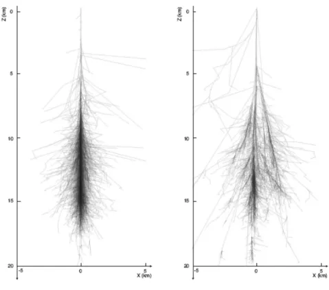
The detection of gamma rays is an indirect process, in which the earth’s atmosphere is used as a calorimeter. When a gamma ray enters the atmosphere, it interacts with the air molecules and induces a chain reaction, a so-called air shower (Grieder, 2010) of secondary particles. Simulated air showers are displayed in Figure 1. Air showers can be seen by Cherenkov telescopes by making use of Cherenkov light (Cherenkov, 1934), which is blue light emitted by air showers. The blue light is emitted in very short flashes, lasting only some microseconds, and cannot be seen by the human eye. Cherenkov telescopes, however, collect the blue light flashes and direct them into a camera, which creates images of the air showers. The imaging is done in such a way that the shape of a shower as seen in Figure 1 remains in the image. The camera and thus the quality of the images depends on the telescope one is using. The cameras of the MAGIC and FACT telescopes and some sample images are introduced in the following chapters.

The problem with the data collection process is that not only the interesting gammas induce particle showers. Hadrons also induce them and they emit Cherenkov light just like the gamma-induced showers, which is also collected by Cherenkov telescopes. To analyse gamma events, it is thus necessary to separate gamma rays from the hadronic background. The separation is done using classification techniques described in later Chapters.

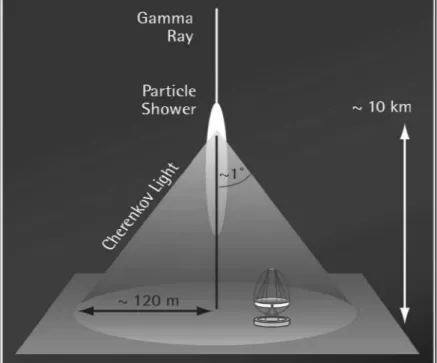
The whole data collection process with Cherenkov telescopes can be seen in Fig- ure 2.

2.2 MAGIC

The two MAGIC telescopes (MAGIC Collaboration, 2014), which are two of the largest Cherenkov telescopes in the world with a mirror diameter of about 17

(13)

2 MOTIVATION 11

Figure 1: Simulated air showers of a gamma ray (left) and a proton (right)(Sidro Martin, 2008)

meters, are situated on the mountain Roque de los Muchachos on the Canary island of La Palma. In spite of being so large, the telescopes are highly mobile.

They can be directed to every spot in the sky in about 25 seconds (Ferenc, 2005).

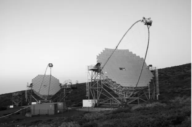
Figure 3 shows the older MAGIC I telescope in the back and the newer MAGIC II telescope, which began operating in 2009 and features an improved camera (Hsu et al., 2007) and improved mirrors (Backes et al., 2007), in the front. As can be seen in the Figure, the telescopes mainly consist of parabolic mirrors, which collect and focus the Cherenkov light emitted from air showers, and a camera, which converts the collected light into photo electrons.

At the time of our analysis of MAGIC data, the MAGIC I camera consisted of 578 hexagonal photo multiplier tubes (PMTs, see e.g. Errando, 2006), but has been

(14)

Figure 2: The data collection process with Cherenkov telescopes. A particle enters the atmosphere and induces a particle shower which sends out Cherenkov light.

The light can be detected by a Cherenkov telescope. (Hadasch, 2008)

upgraded in 2012 to achieve full technical homogeneity between the two telescopes.

Since then, both cameras consist of 1039 PMTs (Nakajima et al, 2013). We did not use the data from the new camera, as we used data from the FACT telescope at the time it was installed. This had several reasons, which we point out below.

PMTs convert light into photo electrons. The number of photo electrons triggered in a PMT depends on the intensity of the light registered in that PMT. To minimize the space between PMTs, they are complemented by hexagonal cones, so called Winston Cones. The combination of Winston Cone and PMT is called a pixel. A schematic view of the older MAGIC I camera and the new camera layout can be seen in Figure 4.

(15)

2 MOTIVATION 13

Figure 3: The two MAGIC telescopes. The older MAGIC I telescope (left) and the newer MAGIC II telescope (right) (MAGIC-Homepage, 2010).

2.3 FACT

The FACT telescope seen in Figure 5 is a single dish telescope also located on the MAGIC site. It is based on one of the former HEGRA telescopes and has a mirror plane of 9.5 sqm. The name FACT stands for First G-APD Cherenkov Telescope, which also describes its main characteristic: FACT is the first imaging Cherenkov telescope to use Geiger-mode avalanche photodiods (G-APDs) instead of photomultiplier tubes (PMTs), which need a lower voltage and have a higher photon detection efficiency (FACT Collaboration, 2014).

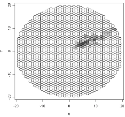
The FACT camera consists of 1440 G-APDs, that is, 1440 pixels. A schematic

(16)

Figure 4: The cameras of the two MAGIC telescopes with numerized pixels. The older MAGIC I camera on the left and the newer MAGIC II camera on the right, which is also used in the MAGIC I telescope now. (MAGIC-Homepage, 2010).

view of the FACT camera with a simulated sample event can be seen in Figure 6.

Although technical details of the FACT telescope differ from the MAGIC telescopes, the aim and analysis of the experiments are basically the same: The detection of highly energetic gamma rays.

2.4 The Analysis Chain

The analysis chain used in the two expermiments MAGIC and FACT is basically the same. Besides the steps mentioned here, there are some more, which are mandatory and not interchangable and therefore not of interest here. For example the calibration of images.

(17)

2 MOTIVATION 15

Figure 5: The FACT telescope. One can see the mirror plane and the camera embedded in the white metal cylinder. (MAGIC-Homepage, 2010).

2.4.1 Image Cleaning

When recording Cherenkov light with the MAGIC or FACT telescopes not only Cherenkov-photons are recorded. Background light emitted for example by nearby cities or the illuminated night sky (moon and stars) are also recorded. This background light is not to be confused with the hadronic background events. For better differentiation from background events we call the background light here noise. The noise is present in all camera images, regardless if it is a signal event or a background event. At full moon this noise can be so strong that taking data is almost impossible.

(18)

Figure 6: A sample image of an air shower induced by a simulated gamma ray.

The greyscale shows the intensity of light in each pixel. The darker a pixel is, the more Cherenkov light photons have been collected.

Since the noise is always present, it is inherent in all images recorded. The actual shower is thereby overlapped by the noise and creates an image which has positive intensities in all pixels, with the intensity being largest where the actual shower is recorded. This can be seen on the left hand side of Figure 7. Would further steps of the analysis be used on this uncleaned picture, the results would be strongly biased.

For this reason a so-called image cleaning step is necessary. In this step, one tries to decide which of the pixels belong to the actual shower and which ones only contain noise. The intensity of pixels, which are thought to only contain noise,

(19)

2 MOTIVATION 17

are set to 0. This can be seen on the right hand side of Figure 7. Here an image cleaning has been used to cut out the actual shower and suppress the noise.

Although the shower can usually be seen by the naked eye in most images, the image cleaning is not trivial. Especially on the edge of showers it is difficult to decide which pixels should be suppressed. Especially difficult is the image cleaning in images, which recorded events of smaller energy, because they emit less Cherenkov photons than events of higher energy, which leads to lower intensities in shower pixels.

The image cleaning in Figure 7 is the one typically applied in MAGIC, which is also used in FACT. The image cleaning done on the data we use consists of these steps (cf. Thom, 2009):

1. Determine Core Pixels: Pixels with an intensity larger than a thresholdc_high 2. Determine Used Pixels: Pixels with an intensity larger than a thresholdclow,

which are neighbours of Core Pixels.

3. Set intensity of all other pixels to 0.

4. Set intensity of isolated Core Pixels to 0, that is Core Pixels with neighbours all having intensity 0.

The thresholdsc_high andc_lowhave to be chosen reasonably and are very different for the two telescopes. For MAGIC the standard values arec_high = 8.5 andc_low = 4.5.

For FACT the values have to be much higher, because the G-APDs used are able to detect more light and thus also more background.

It is possible that there are some separate areas of intensity greater than 0 after

(20)

the image cleaning. We call these areas islands. The biggest island in terms of used pixels is called Main Island, the other are called Sub Islands.

In an extended image cleaning also time information is considered.

We do not change the image cleaning in this work, but it should be kept in mind that the image cleaning is an important step in the analysis and shows large room for improvements. See Deiters (2013) for example for a comparison of filter techniques and their influence on the image cleaning and the further analysis.

Figure 7: A sample image before (left) and after (right) the image cleaning. In this case the number of islands in the image is 1.

2.4.2 Quality Cuts

Quality Cuts (cf. Bretz, 2006) filter events, which are either impossible to classify (for example because they are too small) or which cannot possibly be signal events.

Only events which fulfill the following conditions are kept in the data set:

(21)

2 MOTIVATION 19

Number of islands < 3. It is known that signal events cannot have more than two islands.

Number of pixels>5. The image must consist of more than five pixels with an intensity greater than zero after the image cleaning. Else it is too small to make any justifiable assertions about it.

Leakage < 0.3. That means that more than 70% of the shower has to be within the camera plane. This is measured by the Hillas parameter Leakage, see below.

See Bretz (2006) for more, less intuitive and not interpretable quality cuts.

2.4.3 Variable Extraction

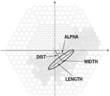
In order to classify the images into background and signal, proper classification variables have to be extracted from the raw images. The currently used variables are so-called Hillas parameters, which were first introduced by Hillas (1985) and extended for example by stereoscopic features introduced by Kohnle et. al. (1996) and variables describing the time evolution of a shower (e.g. Bastieri, 2005). The idea underlying the original Hillas variables is to fit an ellipse to a shower image and use the parameters of the ellipse along with some additional features as variables in the classification. This can be seen in Figure 8, where a few sample Hillas variables are displayed. The Hillas variables are explained in more detail in Chapter 4.2, where we also construct new variables to complement the currently used Hillas variables.

(22)

Figure 8: Some Hillas variables from fitting an ellipse.

(source: http://ihp-lx.ethz.ch/Stamet/magic/parameters.html)

2.4.4 Gamma-Hadron-Separation

With the Hillas variables extracted in the previous step, a classification is done to separate gamma ray events from hadronic background events. The separation is important, as a pure gamma sample is necessary to draw conclusions about the source one is observing.

Usually in the MAGIC and FACT experiments random forests (Breiman, 2001) with some minor changes described in Albert et al. (2008) are used for the classification.

The gamma-hadron-separation is the central aspect of this work. It is described in more detail in Chapter 3, where a method for optimizing the discrimination threshold of a random forest is introduced.

(23)

2 MOTIVATION 21

2.4.5 Unfolding of Energy Spectra

A central goal of the analysis of MAGIC and FACT data is to reconstruct energy spectra of the observed source, that is the distribution of the energy of gamma ray particles emitted by the source.

Energy spectra are usually estimated by histograms of the estimated energy of gamma particles. There are several uncertainties in estimating such a spectrum.

For example the energy reconstuction of a particle is not exact, but only an estimation. Because of this the true energy of a particle is not always reconstructed accurately, so that a particle can be falsely sorted into a wrong energy range.

The most important uncertainty in this work comes from the difficult classification of signal and background. For the estimation of energy spectra, the data one estimates it from has to be a very pure gamma sample. Classification errors in the gamma-hadron-separation make it difficult to estimate the true energy spectrum and leads to a biased estimation. This means firstly that the classification has to be done as exactly as possible and secondly that the estimated spectrum has to be bias-corrected as long as the gamma-hadron-separation is not perfect.

The bias-correction is done using an unfolding procedure implemented in the unfolding program TRUEE (Milke et al., 2012). The idea of the unfolding is the following: The true energy distribution, or more exactly, its density f(x), is assumed to be folded by a kernel functionA(y, x) into the observed distribution with densityg(y). This can be written using the Fredholm integral equation (Fredholm, 1903),

g(y) = Z

A(y, x)f(x)dx+b(y)

where also a known background density b(y) is added additively. Considering

(24)

discrete or classed distributions this becomes a lot easier. Let g₁, ..., g_k be the relative number of observations in thek observed energy classes andf₁, ..., f_m the true probabilities of the m energy classes (the binning in the observed and true distributions can be different), then the above Fredholm integral can be rewritten using ak×m-Matrix A and vectors g = (g₁, ..., g_k)^T and f = (f₁, ..., f_m)^T:

g =Af +b

This is a well-known linear model with the vector of observationsg, design matrix A, parameter vector f and vector of errors b. Thus, the unfolding of the energy spectrum is an estimation of the vector f, where the vector g is observed and the transition matrix A is determined on simulated data and then used on real data. The estimation off can be done using ordinary least squares, but experience shows that such estimations have large fluctuations. Therefore, more sophisticated approaches are used in TRUEE, such as the usage of B-Splines and a penalized minimization, which shows high resemblance to Ridge Regression.

The whole theoretical foundation of unfolding can be seen in Blobel (2010) and the exact procedure used in TRUEE can be seen in Milke (2012).

(25)

2 MOTIVATION 23

2.5 MAGIC and FACT Data

In this Chapter we describe the data we use in this work.

2.5.1 The FACT Data Set

The FACT data set we are using is a synthetic data set consisting of real background data and simulated signal. The real background is taken from the Crab Nebula and therefore consists also of gamma rays from this source. The background data is thus not only pure background, but also contains gamma events.

However, the gamma count in this data is expected to be very small, as the signal to background ratio is usually about 1:1000 (Weekes, 2003). Additionally, real background also consists of some gamma rays, only that they are not from the source one is observing. Also, due to the relatively small number of events we use only a signal to background ratio of 1:100 in our analyses, so that the number of gammas in the background is so small that they should not make a difference.

That is why using this data as background should not be much of a problem. The background data set consists of 12,768 events. The simulated data consists only of gamma events. The simulations are from an early stadium of simulations and represent data from the Crab nebula. The signal data set has 12,500 events.

The combined, synthetic data set thus consists of 25,283 events. However, this is before the quality cuts described in Chapter 2.4.2 are applied. After the application of quality cuts, 6,707 real background events and 6,472 simulated signal events remain in the data set, for a total of 13,179 events.

The FACT data set includes data from different analysis steps. We have uncleaned and cleaned camera pixel data available as well as the Hillas variables. That is

(26)

why we can easily calculate new variables on this data set from the camera data and combine them with Hillas variables. However, the drawback of this data is that the data set is relatively small, so that it is difficult to make analyses with a real signal to background ratio. We also do not have information about the true or estimated energy of observations in this data.

2.5.2 The MAGIC Data Set

The MAGIC data we use here is synthetic data consisting of real background and simulated signal events. The data was taken by the two MAGIC telescopes operating in stereoscopic mode. The data set consists of 652,935 simulated gamma events and 357,850 hadronic background events, for a total of 1,010,785 events.

We only have Hillas parameters available in this data, along with a variable called estimated energy, which includes for each observation the energy estimated by a random forest regression (not to be confused with the random forest used for the gamma-hadron-separation).

2.6 High Class Imbalance and the Consequences

It is known that in real MAGIC and FACT data the ratio between signal and background is very unfortunate. Signal events are known to be about 100 to 1000 times less frequent than background (Weekes, 2003). This poses problems. First of all the classification becomes exceptional difficult and the search for gammas becomes looking for needles in a haystack. Especially often used measures of quality for classification like the accuracy, that is the ratio of correctly classified observations, are much less meaningful. With a ratio of signal to background of

(27)

2 MOTIVATION 25

1:1000, a classifier, which always classifies every event as background, will give an accuracy of 99.9%. The ratio also poses a problem for the reconstruction of energy spectra. The first step of the reconstruction is estimating how many signal events there are in the data. This becomes very difficult if too much background is classified as signal. ROC curves for example, which are often used in classification problems, are also not that meaningful here, because a larger area under the curve does not necessarily mean that the signal is estimated better.

We also have a problem with training data. As we do not know the exact signal to background ratio in real data, any number of signal and background events can or has to be used as training data, but the ratio has to be taken into account when assessing the quality of the classification. With a ratio of 1:1 in the training data for example, the number of falsely classified background events has to be very low on this data to achieve a pure sample of signal events on real data and keep the error of the estimation of the number of signal events as low as possible. That is why we want the falsely classified background to be in general very small, while we want to minimize the error we make on signal events.

2.7 Aim

The aim of this work is to improve upon the current MAGIC and FACT analysis chains. Some methods used in this analysis chain are either old for Cherenkov astronomy standards or heuristical or both.

The Hillas parameters for example were introduced by Hillas in 1985, which was at the very beginning of Cherenkov astronomy. They were a first attempt to describe shower images and were not specifically designed to find differences between the gamma ray signal and the hadronic background. In other words they were not

(28)

constructed with the aim of the analysis in mind. As stated above, the aim of the analysis chain is the reconstruction of energy spectra. That means the whole analysis is only done for that aim to estimate the true energy spectrum of a source one is observing.

This has some consequences. In the gamma-hadron-separation step for example, classification methods (here usually random forests (Breiman, 2001; Albert et al., 2008)) are used to separate the gamma ray signal from the hadronic background.

There are many quality measures for classification methods, for example simply the classification accuracy, which is the ratio of correctly classified observations.

There is also the false positive rate (FPR) and true positive rate (TPR), also known as sensitivity and specificity, with the FPR being the ratio of falsely classified background observations and the TPR being the ratio of correctly classified signal observations. The two values are often considered together in ROC curves (Fawcett, 2006).

In our astronomical setting, however, where the overall aim of the analysis is to reconstruct energy spectra, considering only such quality measures can be mislead- ing. For example increasing the accuracy of the classification even to very high values does not necessarily mean an improvement of the reconstruction of energy spectra. One reason for this is the very unfortunate signal to background ratio, introduced above.

The aim of this work is thus to improve upon the currently used analysis chain with respect to the objective of the analysis, that is the reconstruction of energy spectra. As we will see, the reconstruction can be considered as an estimation task. We can thus use quality measures for estimators, here especially the MSE, to measure the quality of our classification.

(29)

2 MOTIVATION 27

In a first step we use this MSE to optimize a discrimination threshold in the outcome of a random forest to improve the classification in such a way that the reconstruction of energy spectra is improved.

In a second step we construct new variables for the classification to improve upon the Hillas parameters. The new variables are constructed by fitting bivariate distributions to shower images and determining the distance between the observed and fitted distributions. As stated above, it is important in our context to maintain a very low FPR, for being able to properly estimate energy spectra. We investigate if the newly constructed variables improve upon the TPR while maintaining a very low FPR.

In a third step the threshold optimization and variable construction are used together. In this step we examine if the suggested methods in this work lead to improvements of the analysis chains of the two telescopes.

(30)

(31)

3 THRESHOLD OPTIMIZATION 29

3 Threshold Optimization

In this chapter we optimize the threshold in the outcome of a random forest to improve upon the estimation of the number of signal events in a data set. We begin by stating the problem setup, then describe the method used to optimize the threshold and finally apply the method to synthetic MAGIC data. The contents of this chapter can also be seen in Voigt et al. (2014) and partly in Voigt & Fried (2013).

3.1 Problem setup

The problem we are facing is a binary classification problem. Some of the features described here are distinctive properties of our astrophysical setting. We have a random vector of input variables X = (X₁, ..., X_m)^T and a binary classification variable Y. We denote the joint distribution of X and Y with P(X, Y). We neither know this distribution nor can we make any justifiable assumptions about it. Additionally, in our application it is not possible to draw a training sample from the joint distribution. We are, however, able to draw samples from the conditional distributions P(X|Y = 0) and P(X|Y = 1). Thus, we have independent realizations (x₁,0), ...,(x_m_0·,0) and (x_m_0·₊₁,1), ...,(x_m_1·_+m_0·,1) from the respective distributions with sizes m_0· and m_1·, respectively, and m=m_0·+m_1·.

Based on these samples a classifier is trained. A classifier such as a random forest or logistic regression can be interpreted as a function f : R^m → [0,1]. For a random forest for example the output of this function is the fraction of trees which voted for Y = 1. For a final classification into 0 and 1 we need a threshold c, so

(32)

that

g(x;c) =







0, if f(x)≥c 1, if f(x)< c

. (1)

We considerf to be given and only vary cin this Chapter.

We call the above samples (x₁,0), ...,(x_m_0·,0),(x_m_0·+1,1), ...,(x_m,1) the training data. As stated above, each of the m observations belongs to one of two classes, where m1· is the number of observations in class 1 and m0· is the number of observations in class 0. In the following, observations of class 1 are called positives and observations of class 0 are called negatives.

In addition to the training data, we have a sample of actual data to be classified, x^∗₁, ...,x^∗_N, for which the binary label is unknown. This data consists of N events with N_1· and N_0· being the unknown random numbers of signal and background events in this data. N,N1·andN0·are therefore random variables. This means our actual data, which we want to analyse, contains a random number of observations.

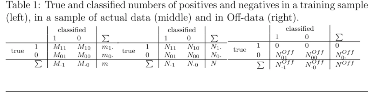
For a given threshold c, we denote the numbers of observations in the training data after the classification as M_ij, i, j ∈ {1,0}, where the first index indicates the true class and the second index the class as which the event was classified by (1). We can display these numbers in a 2×2 table. With N_ij, i, j ∈ {1,0} defined analogously we get a similar 2×2 table for the actual data, see Table 1.

Table 1: True and classified numbers of positives and negatives in a training sample (left), in a sample of actual data (middle) and in Off-data (right).

classified

1 0 P

true 1 M11 M10 m1·

0 M01 M00 m0·

P M·1 M·0 m

classified

1 0 P

true 1 N11 N10 N1·

0 N01 N00 N0·

P N·1 N·0 N

classified

1 0 P

true 1 0 0 0

0 N₀₁^{Of f} N₀₀^{Of f} N_0·^{Of f} P N_·1^{Of f} N_·0^{Of f} N^{Of f}

(33)

It is obvious that we do not know the numbers in the first two rows of the table of the actual data as we do not know the true numbers of positives and negatives N1· and N0·.

As we can see above, N1· is considered to be a random variable and our goal is to estimate, or perhaps better predict, the unknown realization of N1·. The same applies for the numberN0·. That is why we consider all the following distributions to be conditional on these values.

As explained above, we are only able to draw samples from conditional distributions. The difference between sampling from the joint distribution and sampling from the conditional distributions is that the marginal probability P(Y = 1) can be estimated from samples from the joint distribution, but not from samples from the conditional distributions. This is because the samples from the conditional distributions are obtained from Monte Carlo simulations, where the sample sizes have to be set manually before the simulation.

To estimate the number of signal eventsN1·we have additional information in the form of Off data available. In our astrophysical setting we collect Off data by observing a source-free position in the sky so that only background data is observed.

This can be seen on the right hand side of Table 1. Technically speaking Off data represents another way to sample from the conditional distribution P(X|Y = 0).

The sample size N_0·^{Of f} in this data is assumed to be a random variable with the same distribution as the unobservableN0·. This is a reasonable assumption in our asrophysical setting, as background can be considered homogeneous, so that for equal observation time and collection area, the background should be the same,

(34)

short of random effects. N_0·^{Of f} can therefore be used to assess the amount of background in our data, that is N0·, and is used in estimators derived from a classification (see Chapter 3.2). Through classification of the N_0·^{Of f} Off-Events we get the number of correctly and falsely classified observations in this data, N₀₀^{Of f} and N₀₁^{Of f}, see Table 1. In our astronomical setting we get Off data by observing a source-free position in the sky, from which we know that no signal events are emitted. For more information about Off data see Chapter 3.4.

To summarize, we have three data sets:

Training data, containing a manually fixed amount of positives, m1·, and negatives, m_0·.

Actual data, of which we want to estimate the number of positivesN1·.

Off data, containing only negatives, where the number of negatives N_0·^{Of f} is random and has the same distribution as the number of negatives in the actual data.

Our main goal is to estimate the number of positives in the actual data,N1·. This is not an easy task as P(Y = 1) is known to be very small, of size around 1/100 or 1/1000. Because of this fact and because of the other characteristics of our application mentioned above, standard estimators of N_1· or P(Y = 1) will fail to estimate these values accurately.

We make some additional assumptions: We assume that theN_i1, theN₀₁^{Of f} and the M_i1, i ∈ {1,0} are independent and (conditionally) follow binomial distributions.

These assumptions also follow directly from an assumed multinomial distribution

(35)

for the entries of Table 1:

N₀₁|_N_0·_=n_0· ∼Bin (n0·, p₀₁), (2)

N₁₁|_N_1·_=n_1· ∼Bin (n_1·, p₁₁), (3)

N₀₁^{Of f}|_N^{Of f}

0· =n^{Of f}_0· ∼Bin

n^{Of f}_0· , p₀₁

, (4)

M₀₁∼Bin (m_0·, p₀₁), (5)

and

M₁₁∼Bin (m1·, p₁₁), (6)

with some probabilities p₀₁ and p₁₁. As estimators for these two probabilities we use the True Positive Rate (T P R), which is also known as Recall or (signal) Efficiency, and the False Positive Rate (F P R)

T P R= M₁₁

m_1· (7)

and

F P R= M₀₁ m0·

. (8)

Obviously, both rates can only take values in the interval [0,1] and they depend on the discrimination threshold c, as M₁₁ and M₀₁ depend on it. When choosing

(36)

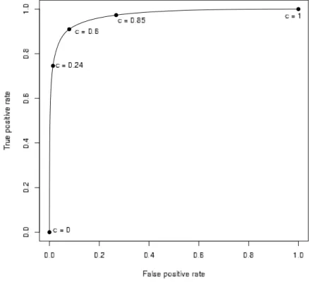
Figure 9: ROC curve for the MAGIC data. The higher in the top left corner the curve lies, the better is the classification. This curve shows that the classification in the MAGIC analysis chain is quite good. The problem is how to finally choose the threshold.

an appropriate c, a high value of T P R and a low value of F P R are desired.

These two requirements, however, are contradictory, because a high value of the threshold leads to high values ofT P RandF P Rand vice versa. Figure 9 depicts a Receiver Operating Characteristic (ROC) curve (see Fawcett, 2006), which shows the T P R and F P R when altering the discrimination threshold. As we will see in the following Chapter, these two values are important in the estimation of the number of positives.

(37)

3.2 Estimation of the true number of positives

As stated above the estimation of the true number of positives N_1· is the main aim of our analysis. Depending on the individual problem such an estimator can look quite differently. For the given application of VHE gamma-ray astronomy, it is known that an irreducible portion of the recorded negatives will be misclassified (Sobczynska, 2007; Maier and Knapp, 2007). Thus, the number of positives is estimated via a difference estimator, as the number N₀₁ of misclassified negatives in actual data can be approximated by the numberN₀₁^{Of f} of misclassified negatives in real Off data. According to Li and Ma (1983) the estimator

N˜_1·^LM=N −N_0·^{Of f} (9)

is the Maximum Likelihood estimator in this situation if a Poisson distribution is assumed forN1·,N0·and N_0·^{Of f} and if we consider that the observation times ofN and N0· are the same and no classification is done. This estimator is uncondition- ally unbiased, E

N˜_1·^LM −N1·

= 0, but a major problem of it is that its standard error is usually very high in case of a large class imbalance. The mean square error of this estimator is

MSE N˜_1·^LM

= E

N˜_1·^LM−N1·

2

= Var (N0·) + Var

N_0·^{Of f}

.

For example, if we assume independent Poisson distributions N_1·∼P ois(λ₁),

N0·∼P ois(λ₀),

(38)

and

N_0·^{Of f} ∼P ois(λ₀)

a signal to background ratio of 1:100 implies that the root mean square error of estimator (9) then is√

100λ₁+ 100λ₁ =√

200λ₁. In case ofλ₁ = 1000 the number of signal events would be estimated with a standard error of about 450, which is rather high. Additionally, the imbalance in our application is usually much worse than 1:100.

3.2.1 Estimation with known classification probabilities

The above estimation does not consider a classification before estimating the number of signal events. The idea of a classification in this situation is to suppress a large amount of the background events to receive a classified dataset with a more desirable signal to background ratio. If p₁₁ was known, a corresponding estimator, which takes classification and the above mentioned binomial assumptions into account, would be

N˜_1· = 1 p₁₁

N_·1−N₀₁^{Of f}

. (10)

Analogously to the estimator in equation (9), this quantity takes the difference between N·1 and N₀₁^{Of f} as an estimate for N₁₁ and multiplies this with _p¹

11 to compensate for the classification error in the signal events. It translates into the estimator in equation (9), when p₁₁ =p₀₁ = 1. Per construction this quantity can give negative results thoughN1·is positive. Since we cannot achieve zero variance of the estimator, we cannot achieve an unbiased estimation when restricting its range to positive values. Because of the assumption thatN₀₁ andN₀₁^{Of f} follow the

(39)

same distribution we have E( ˜N1·−N1·) = 0, justifying usage of ˜N1·. Of course, when the results are to be interpreted in the application context, one might want to replace negative estimates by 0, but the corresponding estimator would be biased at least in case of zero or small values of N1·.

Obviously, the estimators in (9) and (10) cannot be used in problems where one does not have access to an Off data set. In this case, an alternative is for example the estimator N·1m1·

M·1. The following calculations have to be adapted to this estimator. In our application, however, this estimator cannot be used, as m_1. has to be set manually for the Monte Carlo simulations, so that using this estimator does not make sense.

Since we want to estimate the number of positives as exactly as possible we want to assess the quality of the estimator ˜N1·. A standard measure of the quality of an estimator is the mean square error (MSE). As in applications we usually have fixed samples in which we want to estimate N1·, we calculate the MSE conditionally on N1·,N0· andN_0·^{Of f}. The problem of high inaccuracy of the estimator ˜N_1·^LM remains in this situation, as its conditional bias is very high, although its variance is 0.

The MSE simplifies to the variance for unbiased estimators, so it is of interest if the estimator in (10) is unbiased for every fixed number of gamma eventsN1·, that is whether

Bias

N˜1·|N1·, N0·, N_0·^{Of f}

= E

N˜1·|N1·, N0·, N_0·^{Of f}

−N1·

equals 0, where E

N˜_1·|N_1·, N_0·, N_0·^{Of f}

is the conditional expectation of the estimator ˜N1· given the values of N1·, N0· and N_0·^{Of f}.

(40)

Under the binomial assumptions made in the previous Chapter (equations (2) - (6)) we can easily calculate the conditional expectation of ˜N1·:

E

N˜1·|N1·, N0·, N_0·^{Of f}

= E 1

p₁₁

N·1−N₀₁^{Of f}

|N1·, N0·, N_0·^{Of f}

= 1 p₁₁E

N₁₁+N₀₁−N₀₁^{Of f}|N_1·, N_0·, N_0·^{Of f}

= 1 p₁₁

N1·p₁₁+N0·p₀₁−N_0·^{Of f}p₀₁

=N_1·+ p₀₁ p11

N_0·−N_0·^{Of f}

The conditional bias of ˜N1· from equation (10) thus is Bias

N˜1·|N1·, N0·, N_0·^{Of f}

= p₀₁ p₁₁

N0·−N_0·^{Of f}

. (11)

This bias matches with what one would expect intuitively as it is small for p01

small and for p₁₁ high and it reaches zero if no background is falsely classified or if the number of background events in the Off data is the same as in the actual data.

A standard measure for the quality of an estimator is the (conditional) MSE given by

MSE

N˜_1·|N_1·, N_0·, N_0·^{Of f}

= E

N˜_1·−N_1·2

|N_1·, N_0·, N_0·^{Of f}

= Bias

N˜1·|N1·, N0·, N_0·^{Of f}2

+ Var

N˜1·|N1·, N0·, N_0·^{Of f} . (12) This variance term can easily be calculated by again using the assumption that

(41)

N₁₁,N₀₁ and N₀₁^{Of f} are independent and follow binomial distributions:

Var

N˜1·|N1·, N0·, N_0·^{Of f}

= Var 1

p₁₁

N·1−N₀₁^{Of f}

|N1·, N0·, N_0·^{Of f}

= 1 p²₁₁Var

N₁₁+N₀₁−N₀₁^{Of f}|N1·, N0·, N_0·^{Of f}

= 1 p²₁₁

N1·p11(1−p11) +

N0·+N_0·^{Of f}

p01(1−p01)

=N1·

1 p₁₁ −1

+p01−p²₀₁ p²₁₁

N0·+N_0·^{Of f}

(13)

Using equations (13) and (11) the MSE in (12) becomes MSE

N˜1·|N1·, N0·, N_0·^{Of f}

= p²₀₁ p²₁₁

N0·−N_0·^{Of f}2

+N1·

1 p₁₁ −1

+ p₀₁−p²₀₁ p²₁₁

N0·+N_0·^{Of f} .

(14)

3.2.2 Estimation with Unknown probabilities

The above equation (14) depends on the values ofp11 andp01. As we do not know these values we have to estimate them. Consistent estimators for these values are T P R and F P R (equations (7) and (8)). Using T P R as an estimator for p11 in equation (10) we get the realistic estimator

Nb_1·= m_1·

M₁₁

N_·1−N₀₁^{Of f}

= 1

T P R

N_·1−N₀₁^{Of f}

. (15)

As T P R and F P R are consistent estimators of p₁₁ and p₀₁, and the sample sizes m1· and m0· are usually large (> 10⁵), using the estimators instead of the true

(42)

probabilities should only lead to a small difference. By estimating p₁₁ with T P R and p₀₁ with F P R in equation (14) we get the estimate

MSE[

N˜_1·|N_1·, N_0·, N_0·^{Of f}

= F P R² T P R²

N_0·−N_0·^{Of f}2

+N1·

1 T P R −1

+F P R−F P R² T P R²

N0·+N_0·^{Of f} . (16)

Note that ˜N_1·is not a feasible estimator sincep₁₁ is unknown. Instead we propose Nb1·, but under our binomial assumptions neither the expectation nor the MSE of Nb_1· exist, since the term E

1 M11

is involved, which is infinite if P(M₁₁ = 0) >

0. The binomial distribution, however, is only an approximation to reality as in practice we can simulate data untilM₁₁>0. We find it hard to provide a realistic model for this process and use MSE

N˜1·|N1·, N0·, N_0·^{Of f}

as a measure of quality also for the estimator Nb_1· deduced from ˜N_1·. In our experience this gives good results, see Chapter 3.5.

As we see in the following Chapter, equations (15) and (16) can be used in an iter- ative manner to find an optimal discrimination threshold. Therein equation (16) is treated like the total misclassification costs in the thresholding method as value to be minimized over the threshold.

3.3 Minimizing the MSE to choose the threshold

As stated above, the valuesT P Rand F P Rdirectly depend on the discrimination threshold. If the number of positivesN1· was known we could minimize the MSE in equation (16) over all possible thresholds and thus find the one with which the

(43)

number of positives can be estimated best.

For simulations with a known ratio of positives and negatives, this is shown in Figure 10. It illustrates the MSE, calculated with equation (16) and depending on the threshold, for a fixed number of 5000 positives and different numbers of negatives. The solid curve, for a ratio of 1:50, that is 250000 negatives, is rather flat in comparison to the other curves, depicting ratios up to 1:1000. When looking at higher numbers of negatives one can see two major distinctive features. The first one is that the MSE is generally higher. This seems intuitive as it gets more difficult to separate signal and background when the background increases. The second feature is that the optimal value of the threshold approaches zero when the number of negatives is increased. An optimal threshold obviously depends on the class imbalance in the data, that is the ratio between positives and negatives, which is unknown in practice.

In the given astronomical application, this ratio can in general be different for different astrophysical sources the telescope is taking data from and even for different observation times of the same source. Thus using always the same threshold is not recommended. Instead it is desirable to adapt the threshold to the data and to the class imbalance in the data.

The problem here is that, as one knows the sum of positives and negatives N, knowing their ratio is equivalent to knowing the number of positives N1·, the value one wants to estimate. One needs to know N1· to optimize the threshold to find the best estimate of N1·.

An intuitive idea to overcome this problem is to use a rough and easy to compute estimate of N1· to optimize the threshold and then get a better estimate from a new classification. An easy to compute estimate can be obtained by setting the threshold to a fixed default value. According to Figure 10, c= 0.1 seems to be a reasonable initial choice. Using this value for the threshold we estimate N1·, then

(44)

calculate the optimal threshold for this estimate and estimate N1· again for this new threshold. This procedure can be iterated until some convergence criterion is met. This approach leads us to the following algorithm:

1. Set an initial value c for the threshold.

2. Estimate N1· using this threshold and equation (15).

3. Compute a new threshold through minimizing equation (16) over all thresholds using the estimates ˆN1· for N1· and N −Nˆ1· for N0·.

4. If a stopping criterion is fulfilled, compute a final estimate of N1· and stop.

Otherwise go back to step 2.

At this point we need a treatment for negative values of Nb1·, because negative estimates could lead to a negative estimate of the MSE. We then set negative values of (16) to 0. This happens very rarely, as the third term is positive and usually dominant. Please also note that minimization of the MSE takes place only over T P R and F P R, so the estimation of N_1. does not diverge to −∞, because the factors in the other two terms decrease faster in T P R than the second. As a stopping criterion, we require that the change in the threshold from one iteration to the next is below 10⁻⁶.

In the following we refer to this algorithm as the MSEmin method. This method takes both into consideration: The class imbalance problem and the minimization of the MSE, that is, the overall misclassification cost. In the next Chapter we investigate the performance of this algorithm on simulated data and compare it to other possible approaches.

(45)

Figure 10: The MSE plotted against the threshold cfor a fixed number of gamma events and different numbers of hadron-events according to several gamma-hadron- ratios

3.4 Application to astronomical data

In this Chapter we apply the MSEmin method to data from VHE gamma-ray astronomy collected with the MAGIC telescopes.

The MAGIC telescopes on the Canary island of La Palma are a stereoscopic imaging atmospheric Cherenkov telescope system. Its purpose is to detect highly energetic gamma-rays from astrophysical sources. This is done in an indirect way, em- ploying the Earth’s atmosphere as calorimeter: gamma-rays impinging the atmosphere induce cascades of highly energetic charged particles, emitting Cherenkov light (Cherenkov, 1934). For reviews of this research field see Hinton and Hofmann

(46)

(2009), Hinton (2009), and Chadwick et al (2008). One major difficulty is that not only gamma-rays induce such particle showers, but also many other particles summarized as hadrons, which are, for the strongest gamma-ray sources, 100 to 1000 times more common than the gamma-rays of interest (Weekes, 2003; Hinton, 2009). So the gammas, which are the positives in this application, have to be separated from the vast majority of hadrons, which represent the negatives. The separation was enhanced with a significant boost in sensitivity in 2009, when the second telescope was built and the telescope system began observation in stereoscopic mode (Aleksic et al, 2012).

The measurements are conducted in such a way that both the astrophysical sources of VHE gamma-rays and similar sky positions without (known) gamma-ray sources (Off data) are observed, which leads to N events in the data sample, and N^{Of f} events in the Off data sample. For a time-efficient use of the telescopes these observations can even be conducted at once utilizing the false source method (Fomin et al, 1994).

In the MAGIC analysis chain (outlined in Chapter 2.4 or e.g. Firpo Curcoll et al, 2011) the classification is usually done by a random forest (Breiman, 2001;

Albert et al, 2008). For the training of the random forest, Monte Carlo generated gamma-ray events are used as positive examples. The variables used for separation are based on the moment analysis parameters introduced by Hillas (1985), complemented by stereoscopic variables based on Kohnle et al (1996) and variables describing the time evolution of the shower images (Aliu et al, 2009). To obtain realistic distributions of these variables, the whole physical detection process is simulated, from the simulation of the particle showers and the emission of Cherenkov light (Heck and Knapp, 2010) up to the light detection and electronic digitalization process (Carmona et al, 2008; Majumdar et al, 2005). As the involved processes in hadronic shower development are much more complex and the

(47)

telescopes’ efficiency for recording hadron events is about a factor of 10 lower com- pared to gamma induced particle showers, the computation time for a sufficient sample of Monte Carlo simulated hadron events would require many CPU-hours of computation time for a similarly plentiful Monte Carlo sample of hadron events.

Furthermore, the underlying particle physics processes are unaccessible for current precision measurements, so that predictions of different theoretical models differ by 20%–40% (Maier and Knapp, 2007). For these reasons, the negative examples for the training of the random forest are not Monte Carlo generated but taken from measured Off data.

The output of a random forest for each event is the fraction of trees which voted for this observation to be a hadron. A discrimination thresholdchas to be applied in this fraction to finally classify each observation. From applying the trained random forest model f with a fixed discrimination threshold con a test sample of n events, being comprised by m1· Monte Carlo simulated gamma events and m0·

Off data hadron events, the M_ij and thusT P R and F P R can be inferred.

3.4.1 Energy-dependency

As for calculating energy spectra from the number of gamma events, the value of interest is not simply the total number of all gamma events by itself, but the number depending on the energy of the gamma-rays. Therefore we do not compute a single threshold for the whole data set. Instead the data is binned into several classes according to their energy and then the threshold is computed for every bin separately. This can lead to rather different values of the threshold in each energy bin. In reality, the energy of the gamma-rays is neither known nor directly measurable and thus has to be estimated, taking both the limited acceptance and limited energy resolution of the detector into account. This is done by applying

(48)

an unfolding procedure (see Milke et al, 2011, 2012) and possibly also a random forest regression beforehand (Albert et al, 2007). Typically, this is conducted on a logarithmic-equidistant binning in energy, reflecting the detectors energy resolution and the power-law-like decline of event numbers depending on their energy. For this study, we neglect the unfolding procedure to not further complicate the issue and use the term energy for a random forest regression estimate of the true energy for simplicity.

3.4.2 Currently used Recall-methods

The currently used method to find the discrimination threshold, which is called hadronness cut in this application, is a rather simple one. Assuming that the Off data, introduced in Chapter 3.1, represent the real hadron-data exactly, that is N_0· = N_0·^{Of f}, the estimate of N_1· in (15) becomes ˆN_1· = _{T P R}^N¹¹. This estimate is unbiased under the assumption of a binomial distribution in combination with N_0·=N_0·^{Of f}, see (11), and its variance is, see equation (13),

Var

N₁₁ T P R|N1·

= 1

T P R −1

N1·.

Minimizing this variance over all thresholds is equivalent to maximizing T P R. So under the assumption that the Off data perfectly represents the real hadron-data, the best discrimination threshold is the one which maximizes TPR. This results in a threshold where hadronness is equal to 0, classifying all events as gamma and thus receiving T P R= 1.

However, the assumptionN0·=N_0·^{Of f} is very strong, as only their underlying distributions are the same. Therefore, the approach which is used in practice is to set the threshold manually so that the TPR is “high, but not too high”. Often