Cost-Optimal Line Planning ∗
Markus Friedrich
1, Maximilian Hartl
2, Alexander Schiewe
3, and Anita Schöbel
41 Lehrstuhl für Verkehrsplanung und Verkehrsleittechnik, Universität Stuttgart, Stuttgart, Germany
markus.friedrich@isv.uni-stuttgart.de
2 Lehrstuhl für Verkehrsplanung und Verkehrsleittechnik, Universität Stuttgart, Stuttgart, Germany
maximilian.hartl@isv.uni-stuttgart.de
3 Institut für Numerische und Angewandte Mathematik, Universität Göttingen, Göttingen, Germany
a.schiewe@math.uni-goettingen.de
4 Institut für Numerische und Angewandte Mathematik, Universität Göttingen, Göttingen, Germany
schoebel@math.uni-goettingen.de
Abstract
Finding a line plan with corresponding frequencies is an important stage of planning a public transport system. A line plan should permit all passengers to travel with an appropriate quality at appropriate costs for the public transport operator. Traditional line planning procedures proceed sequentially: In a first step a traffic assignment allocates passengers to routes in the network, often by means of a shortest path assignment. The resulting traffic loads are used in a second step to determine a cost-optimal line concept. It is well known that travel time of the resulting line concept depends on the traffic assignment. In this paper we investigate the impact of the assignment on the operating costs of the line concept.
We show that the traffic assignment has significant influence on the costs even if all passengers are routed on shortest paths. We formulate an integrated model and analyze the error we can make by using the traditional approach and solve it sequentially. We give bounds on the error in special cases. We furthermore investigate and enhance three heuristics for finding an initial passengers’ assignment and compare the resulting line concepts in terms of operating costs and passengers’ travel time. It turns out that the costs of a line concept can be reduced significantly if passengers are not necessarily routed on shortest paths and that it is beneficial for the travel time and the costs to include knowledge on the line pool already in the assignment step.
1998 ACM Subject Classification G.1.6 Optimization, G.2.2 Graph Theory, G.2.3 Applications Keywords and phrases Line Planning, Integrated Public Transport Planning, Integer Program- ming, Passengers’ Routes
Digital Object Identifier 10.4230/OASIcs.ATMOS.2017.5
1 Introduction
Line planning is a fundamental step when designing a public transport supply, and many papers address this topic. An overview is given in [18]. The goals of line planning can roughly
∗ This work was partially supported by DFG under SCHO 1140/8-1.
© Markus Friedrich, Maximilian Hartl, Alexander Schiewe, and Anita Schöbel;
licensed under Creative Commons License CC-BY
be distinguished into passenger-oriented and cost-oriented goals. In this paper we investigate cost-oriented models, but we evaluate the resulting solutions not only with respect to their costs but also with respect to the approximated travel times of the passengers.
In most line planning models, a line pool containing potential lines is given. Thecost model chooses lines from the given pool with the goal of minimizing the costs of the line concept. It has been introduced in [5, 26, 25, 6, 12] and later on research provided extensions and algorithms.
Traditional approaches are two-stage: In a first step, the passengers are routed along shortest paths in the public transport network, still without having lines. This shortest path traffic assignment determines a specifictraffic load describing the expected number of travelers for each edge of the network. The traffic loads and a given vehicle capacity are then used to compute the minimal frequencies needed to ensure that all passengers can be transported. These minimal frequencies serve as constraints in the line planning procedure.
We call these constraintslower edge frequency constraints. Lower edge frequency constraints have first been introduced in [24]. They are used in the cost models mentioned above, but also in other models, e.g., in the direct travelers approach ([7, 4, 3]), or in game-oriented models ([15, 14, 20, 21]).
If passengers are routed along shortest paths, the lower edge frequency constraints ensure that in the resulting line concept all passengers can be transported along shortest paths.
Although the travel time for the passengers includes a penalty for every transfer, routing them along shortest paths in the public transport network (PTN) guarantees a sufficiently short travel time. However, routing passengers along shortest paths may require many lines and hence may lead to high costs for the resulting line plan. An option is to bundle the passengers on common edges. To this end, [13] proposes an iterative approach for the passengers’ assignment in which edges with a higher traffic load are preferred against edges with a lower traffic load in each assignment step. Other papers suggest heuristics which construct the line concept and the passengers’ assignment alternately: after inserting a new line, a traffic assignment determines the impacts on the traffic loads ([23, 22, 17]).
Our contribution: We present a model in which passengers’ assignment is integrated into cost-optimal line planning. We show that the integrated problem is NP-hard.
We analyze the error of the sequential approach compared to the integrated approach: If passengers’ are assigned along shortest paths, and if a complete line pool is allowed, we show that the relative error made by the assignment is bounded by the number of OD-pairs. We also show that the passengers’ assignment has no influence in the relaxation of the problem.
If passengers can be routed on any path, the error may be arbitrarily large.
We experimentally compare three procedures for passengers’ assignment: routing along shortest paths, the algorithm of [13] and a reward heuristic. We show that they can be enhanced if the line pool is already respected during the routing phase.
2 Sequential approach for cost-oriented line planning
We first introduce some notation. The public transport network PTN=(V, E) is an undirected graph with a set of stops (or stations)V and direct connectionsE between them. Aline is a path through the PTN, traversing each edge at most once. Aline concept is a set of lines Ltogether with their frequencies fl for alll ∈ L. For the line planning problem, a set of potential lines, the so-calledline pool L0is given. Without loss of generality we may assume that every edge is contained in at least one line from the line pool (otherwise reduce the set
Algorithm 1:Sequential approach for cost-oriented line planning.
Input: PTN= (V, E),Wuv for allu, v ∈V, line poolL0with costscl for alll∈ L0
1 Compute traffic loads we for every edgee∈E using a passengers’ assignment algorithm (Algorithm 2)
2 For every edge e∈E compute the lower edge frequencyfemin:=dCapwe e
3 Solve the line planning problem LineP(fmin) and receive (L, fl)
Algorithm 2:Passengers’ assignment algorithm.
Input: PTN= (V, E),Wuv for allu, v ∈V forevery u, v∈V withWuv>0 do
Compute a set of paths Puv1 , . . . , PuvNuv from uto vin the PTN Estimate weights for the pathsα1uv, . . . , αNuvuv ≥0 withPNuv
i=1 αi= 1 end
forevery e∈E do Setwe:=P
u,v∈V
P
i=1...Nuv: e∈Puvi
αiuvWuv end
of edgesE). If the line pool contains all possible paths as potential lines we call it acomplete pool. For every line l∈ L0 in the pool its costs are
costl=ckm
X
e∈l
de+cfix, (1)
i.e., proportional to its length plus some fixed costs, where de denotes the length of an edge.
Without loss of generality we assume thatckm= 1.
The demand is usually given in form of an OD-matrix W ∈IR|V|×|V|, whereWuv is the number of passengers who wish to travel between the stopsu, v ∈V. We denote the number of passengers as|W|and the number of different OD pairs as|OD|.
The traditional approaches for cost-oriented line planning work sequentially. In a first step, for each pair of stations (u, v) with Wuv >0 the passenger-demand is assigned to possible paths in the PTN. Using these paths, for every edge e∈E the traffic loads are computed. Given the capacity Cap of a vehicle, one can determinefemin:=dCapwe e, i.e., how many vehicle trips are needed along edgeeto satisfy the given demand. These valuesfemin are calledlower edge frequencies. They are finally used as input for determining the lines and their frequencies, Algorithm 1.
The problem LineP(fmin) is the basiccost model for line planning:
min (
X
l∈L0
fl·costl: X
l∈L0:e∈l
fl≥femin for alle∈E, fl∈IN for alll∈ L0 )
. (2)
Cost models (and extensions of them) have been extensively studied as noted in the intro- duction.
Step 1 in Algorithm 1 is called passengers’ assignment. The basic procedure is described in Algorithm 2.
There are many different possibilities how to compute a set of paths and corresponding weightsαiuv; we discuss some in Section 5. In cost-oriented models, often shortest paths through the PTN are used. I.e., Nuv = 1 for all OD-pairs {u, v} and Puv1 = Puv is an
Algorithm 3: Sequential approach for cost-oriented line planning.
Input: PTN= (V, E),Wuv for allu, v∈V, line poolL0 with costscl for alll∈ L0
1 Compute traffic loadswefor every edge e∈E using a passengers’ assignment algorithm (Algorithm 2)
2 Solve the line planning problem LineP(w) and receive (L, fl)
(arbitrarily chosen) shortest path fromutov in the PTN. We call the resulting traffic loads shortest-path based. Furthermore, letSPuv :=P
e∈Puvde denote the length of a shortest path betweenuandv.
In order to analyze the impacts of the traffic loadswe on the costs, note that for integer values offl we have for everye∈E:
X
l∈L0:e∈l
fl≥ we
Cap
⇐⇒Cap X
l∈L0:e∈l
fl≥we,
hence we can rewrite (2) and receive the equivalent model LineP(w) which directly depends on the traffic loads:
LineP(w) mingcost(w) := X
l∈L0
flcostl
s.t. Cap X
l∈L0:e∈l
fl ≥ we for alle∈E (3)
fl ∈ IN for alll∈ L0
We can hence formulate Algorithm 1 a bit shorter as Algorithm 3.
Note that the paths determined in Algorithm 3 will most likely not be the paths the passengers really take after (3) is solved and the line concept is known. This is known and has been investigated in case that the travel time of the passengers is the objective function: Travel time models such as [19] intend to find passengers’ paths and a line concept simultaneously. The same dependency holds if the cost of the line concept is the objective function, but a model determining the line plan and the passengers’ routes under a cost- oriented function simultaneously has to the best of our knowledge not been analyzed in the literature so far.
3 Integrating passengers’ assignment into cost-oriented line planning
In this section we formulate a model in which Steps 1 and 2 of Algorithm 3 can be optimized simultaneously. Our first example shows that it might be rather bad for the passengers if we optimize the costs of the line concept and have no restriction on the lengths of the paths in the passengers’ assignment.
IExample 1. Consider Figure 1a with edge lengthsdAD=dBC = 1,dAB=dDC =M, a line pool of two linesL0:={l1=ABCD, l2=AD} and two OD-pairsWAD= Cap−1 and WBC= 1.
For a cost-minimal assignment we choosePAD= (ABCD),PBC = (BC) and receive an optimal solutionfl1 = 1, fl2= 0 with costs ofgcost=cfix+ 2M + 1. The sum of travel times for the passengers in this solution isgtime= (Cap−1)∗(2M+ 1) + 1.
A
B C
D M
1
M
1
Line l1
Line l2
(a)Infrastructure network for Example 1.
A B
C
D
E Linel1
Linel2
(b)Infrastructure network for Example 3.
Figure 1Example infrastructure networks.
For the assignment PAD = (AD), PBC = (BC) we receive as optimal solution fl1 = 1, fl2 = 1 with only slightly higher costs ofgcost= 2cfix+ 2M+ 2. but much smaller sum of travel times for the passengersgtime= (Cap−1)∗1 + 1 = Cap.
From this example we learn that we have to look at both objective functions: costs and traveling times for the passengers, in particular when we allow non-shortest paths in Algorithm 2. When integrating the assignment procedure in the line planning model we hence require for every OD-pair that its average path length does not increase by more than β percent compared to the length of its shortest path SPuv. The integrated problem can be modeled as integer program (LineA)
(LineA) mingcost := X
l∈L0
fl
X
e∈E
de+cfix
!
s.t. Cap X
l∈L0:e∈l
fl ≥ X
u,v∈V
xuve for alle∈E Θxuv = buv for allu, v∈V X
e∈E
dexuve ≤ βSPuvWuv
fl ∈ IN for alll∈ L0 xuve ∈ IN for alll∈ L0 where
xuve is the number of passengers of OD-pair (u, v) traveling along edgee Θ is node-arc incidence matrix of PTN, i.e., Θ∈R|V|×|E|and
Θ(v, e) =
1 ,ife= (v, u) for someu∈V,
−1 ,ife= (u, v) for someu∈V, 0 , otherwise
buv∈R|V| which containsWuv in itsuth component and−Wuv in its vth component.
Note thatβ = 1 represents the case of shortest paths to be discussed in Section 4. Forβ large enough an optimal solution to (LineA) minimizes the costs of the line concept.
Formulations including passengers’ routing have been proven to be difficult to solve (see [19, 2]). Also (LineA) is NP-hard.
ITheorem 2. (LineA) is NP-hard, even forβ = 1(i.e. if all passengers are routed along shortest paths).
Proof. See [9]. J
The sequential approach can be considered as heuristic solution to (LineA). Different ways of passengers’ assignment in Step 1 of Algorithm 3 are discussed in Section 5.
4 Gap analysis for shortest-path based traffic loads
In this section we analyze the error we make if we restrict ourselves to shortest-path based assignments in the sequential approach (Algorithm 3)andin the integrated model (LineA).
More precisely, we use only one shortest pathPuv for routing OD-pair (u, v) in Algorithm 2 and we setβ= 1 in (LineA). The traffic loads in Step 2 of Algorithm 2 are then computed as
we:= X
u,v∈V:e∈Puv
Wuv. (4)
Assigning passengers to shortest paths in the PTN is a passenger-friendly approach since we can expect that traveling on a shorter path in the PTN is less time consuming in the final line network than traveling on a longer path (even if there might be transfers). It also minimizes the vehicle kilometers required for passenger transport. Hence, shortest-path based traffic loads can also be regarded as cost-friendly. Nevertheless, if we do not have a complete line pool or we have fixed costs for lines, it is still important to which shortest path we assign the passengers as the following two examples demonstrate.
IExample 3 (Fixed costs zero). Consider the small network with stations A,B,C,D, and E depicted in Figure 1b. Assume that all edge lengths are one. There is one passenger from B to E.
Let us assume a line pool with two linesL0={l1=ABCE, l2=BDE}. Since the lines have different lengths their costs differ: costl1 = 3 andcostl2 = 2 (forcfix= 0).
For the passenger from B to E, both possible paths (B-C-E) and (B-D-E) have the same length, hence there exist two solutions for a shortest-path based assignments:
If the passenger uses the path B-C-E, we have to establish linel1 (fl1 := 1, fl2 := 0) and receive costs of 3.
If the passenger uses B-D-E, we establish linel2 (fl1 := 0, fl2 := 1) with costs of 2.
Since in this examplel1 could be arbitrarily long, this may lead to an arbitrarily bad solution.
This example is based on the specific structure of the line pool. But even for the complete pool the path choice of the passengers matters as the next example demonstrates.
IExample 4 (Complete Pool). Consider the network depicted in Figure 1b. Assume, that the edgesBC,CE,BD andDE have the same length 1 and the edgeAB has length. We consider a complete pool and two passengers, one fromAtoE and another one fromB toE.
The vehicle capacity should be at least 2. If both passengers travel viaC, the cost-optimal line concept is to established the dashed linel1 with costscfix+ 2 +. For one passenger traveling viaCand the other one via D, two lines are needed and we get costs of 2cfix+ 4 +. For→0 the factor between the two solutions hence goes to 2ccfix+4+
fix+2+ →2 which equals the number of OD pairs in the example.
The next lemma shows that this is, in fact, the worst case that may happen.
Algorithm 4:Passengers’ Assignment: Shortest Paths.
Input: PTN= (V, E),Wuv for allu, v ∈V forevery u, v∈V withWuv>0 do
Compute a shortest pathPuv fromutov in the PTN, w.r.t edge lengthsd end
forevery e∈E do Setwe:=P
u,v∈V e∈Puv
Wuv
end
ILemma 5. Consider two shortest-path based assignments w and w0 for a line planning problem with a complete pool L0 and without fixed costs cfix = 0. Let fl, l ∈ L, be the cost optimal line concept for LineP(w) and fl0, l∈ L0, be the cost optimal line concept for LineP(w0). Then gcost(w)≤ |OD|gcost(w0).
Proof. See [9]. J
If we drop the assumption of choosing a common path for every OD-pair, the factor increases to the number |W| of passengers. However, if we solve the relaxation of LineP(w) the passengers’ assignment has no effect:
ITheorem 6. Consider a line planning problem with complete pool and without fixed costs (i.e.cfix= 0). Then the objective value of the LP-relaxation of LineP(w) is independent of the choice of the traffic assignment if it is shortest-path based. More precisely:
Let wand w0 be two shortest-path based traffic assignments withg˜cost(w),˜gcost(w0)the optimal values of the LP-relaxations of LineP(w) and LineP(w0). Then ˜gcost(w) = ˜gcost(w0).
Proof. See [9]. J
5 Passengers’ assignment algorithms
We consider three passengers’ assignment algorithms. Each of these is a specification of Step 1 in Algorithm 2. Each algorithm will be introduced in one of the following subsections.
They differ in the objective function used in the routing step, i.e., whether we need to iterate our process or not.
5.1 Routing on shortest paths
Algorithm 4 computes one shortest paths for every OD pair, i.e., all passengers of the same OD pair use the same shortest path.
5.2 Reduction algorithm of [13]
Algorithm 5 uses the idea of [13]. It is a cost-oriented iterative approach. The idea is to concentrate passengers on only a selection of all possible edges. To achieve this, edges are made more attractive (short) in the routing step if they are already used by passengers.
The length of an edge in iteration i is dependent on the load on this edge in iteration i−1, higher load results in lower costs in the next iteration step. This is iterated until no further changes in the passenger loads occur or a maximal iteration countermax_it is reached. When this is achieved, the network is reduced, i.e., every edge that is not used by any passenger is deleted. In the resulting smaller network, the passengers are routed with respect to the original edge lenghts.
Algorithm 5: Passengers’ Assignment: Reduction.
Input: PTN= (V, E),Wuv for allu, v∈V i := 0
w0e:= 0∀e∈E repeat
foreveryu, v ∈V with Wuv>0do
Compute a shortest pathPuvi from uto vin the PTN, w.r.t.
costi(e) =de+γ· de
max{wi−1e ,1}
end
foreverye∈E do Setwei :=P
u,v∈V e∈Puvi
Wuv
end i = i + 1 untilP
e∈E(wi−1e −wie)2< or i>max_it;
Compute a shortest pathPuv from uto vin the PTN, w.r.t.
cost(e) =
(de, wie>0
∞, otherwise Setwe:=P
u,v∈V e∈Puv
Wuv
5.3 Using a grouping reward
Algorithm 6 uses a reward term if the passengers can be transported without the need of a new vehicle. Again, we want to achieve higher costs for less used edges. We reward edges, that are already used by other passengers. In order to fill up an already existing vehicle instead of adding a new vehicle to the line plan we reward an edge more, if there is less space until the next multiple of Cap. To achieve a good performance, we update the edge weights after the routing of each OD pair and not only after a whole iteration over all passengers.
5.4 Routing in the CGN
For line planning, usually a line pool is given. In particular, if the line pool is small, it has a significant impact on possible routes for the passengers, since some routes require (many) transfers and are hence not likely to be chosen. Moreover, assigning passengers not only to edges but tolineshas a better grouping effect. We therefore propose to enhance the three heuristics by routing the passengers not in the PTN but in the co-called Change&Go-Network (CGN), first introduced in [19]. Given a PTN and a line poolL0, CGN=( ˜V ,E) is a graph˜ in which every node is a pair (v, l) of a station v ∈ V and a line l ∈ L0 such that v is contained inl. An edge in the CGN can either be a driving edge ˜e= ((u, l),(v, l)) between two consecutive stations (u, v)∈E of the same linel or a transfer edge ˜e= ((u, l1),(u, l2)) between two different linesl1, l2 passing through the same stationu. In the former case we say that ˜e∈E˜ corresponds toe∈E. We now show how to adjust the algorithms of the previous section to route the passengers in the CGN in order to obtain a traffic assignment in the PTN. For this we rewrite Algorithm 4 and receive Algorithm 7.
We proceed the same way to rewrite the routing step in the repeat-loop of Algorithm 5,
Algorithm 6:Passengers’ Assignment: Reward.
Input: PTN= (V, E),Wuv for allu, v ∈V i := 0
repeat i = i + 1
wei :=wei−1∀e∈E
forevery u, v∈V withWuv>0 do
Compute a shortest pathPuvi fromutov in the PTN, w.r.t.
costi(e) = max{de· 1−γ·(wi−1e mod Cap)/(Cap) ,0}
foreverye∈Puvi−1 do Setwie:=wei−Wuv end
forevery e∈Puvi do Setwie:=wei+Wuv end
end untilP
e∈E(wei−1−wie)2< or i>max_it;
Algorithm 7:CGN routing for Algorithm 4.
forevery u, v∈V withWuv>0 do
Compute a shortest path ˜Puv fromutov in the CGN, w.r.t.
cost(˜e) =
(de if ˜eis a driving edge which corresponds toe
pen if ˜eis a transfer edge, where pen is a transfer penalty end
forevery e∈E do Setwe:=P
˜e∈E:˜
˜
ecorr. toe
Pu,v∈V:
˜e∈P˜uv
Wuv end
where we use
cost(˜e) =
(costi(e) if ˜eis a driving edge which corresponds toe
pen if ˜eis a transfer edge, where pen is a transfer penalty
as costs in the CGN. We still compare the weights wie and wi−1e in the PTN for ending the repeat loop, also the reduction step, i.e., the routing after the iteration in Algorithm 5 remains untouched. For the detailed version see Algorithm 8 in Appendix A.
Finally, we consider Algorithm 6. Here routing in the CGN is in particular promising since a line-specific load is more suitable to improve the occupancy rates of the vehicles. In the routing version of 6 we construct the CGN already in the very first step in the same way as in Algorithm 7. We then perform the whole algorithm in the CGN, but compute the traffic loadswiein the PTN at the end of every iteration in order to compare the weightswie andwi−1e in the PTN for deciding if we end or repeat the loop. For the detailed version see Algorithm 9 in Appendix A.
30 31 32 33 34 35 36 37 38 travel time
1000 1100 1200 1300 1400 1500
costsoptimallineconcept
sp_cgn
rew_cgn red_cgn
sp_ptn
rew_ptn red_ptn
(a)Solution results for a line pool with 33 lines.
28 29 30 31 32 33 34 35 36 travel time
660 680 700 720 740 760 780 800
costsoptimallineconcept
sp_cgn rew_cgn
red_cgn sp_ptn
rew_ptn
red_ptn
(b)Solution results for a line pool with 275 lines.
Figure 2Solution results for a small and a big line pool.
6 Experiments
For the experiments, we applied the models introduced in Section 5 on the data-set from [8], a small but real world inspired instance. It consists of 25 stops, 40 edges and 2546 passengers, grouped in 567 OD pairs. We started with five different line pools of different sizes, ranging from 33 to 275 lines, using [10] and lines based on k-shortest path algorithms. We use a maximum of 15 iterations for every iterating algorithm. For an overview on runtime, see [9].
6.1 Evaluation of costs and perceived travel time of the line plan
We first evaluate a line plan by approximating its cost and its travel times. Both evaluation parameters can only be estimated after the line planning phase since the real costs would require a vehicle- and a crew schedule while the real travel times need a timetable. We use the common approximations:
gcost=P
l∈L0fl·costl, i.e., the objective function of (LineP(w)) and (LineA) that we used before, and
gtime=P
u,v∈V SPuv+ pen·#transfers, describing the sum of travel times of all OD-pairs where we assume that the driving times are proportional to the lengths of the paths and we add a penalty for every transfer.
Comparison of the three assignment procedures
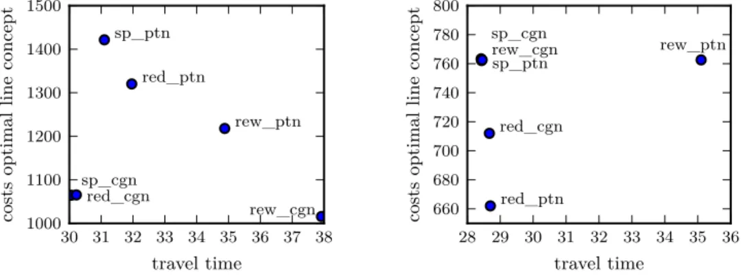
We first compare the three assignment procedures. Figure 2a and 2b show the impact of the assignment procedure for a small line pool (33 lines) and for a large line pool (275 lines).
For both line pools we computed the traffic assignment forShortest Paths,Reduction, and Reward, both in the PTN and in the CGN. This gives us six different solutions, for each of them we evaluated their costsgcostand their travel timesgtime.
Figure 2a shows the typical behaviour for a small line pool: We see thatShortest Path leads to the best results in travel time, i.e., the most passenger friendly solution. Routing in the CGN is better for the passengers than routing in the PTN, the PTN solutions are dominated. Reward, on the other hand, gives the solutions with lowest costs. Also here, the costs are better when we route in the CGN instead of the PTN. Note that the travel time of theRewardsolution in the CGN is almost as good as theShortest Pathsolution.
33 74 125 186 275 line pool size
28.0 28.5 29.0 29.5 30.0 30.5 31.0 31.5 32.0
traveltime
CGN PTN
33 74 125 186 275
line pool size 800
900 1000 1100 1200 1300 1400 1500
costsoptimallineconcept
CGN PTN
Figure 3Travel time and cost ofShortest Pathsolutions for increasing line pool size.
33 74 125 186 275
line pool size 700
800 900 1000 1100 1200 1300 1400
costsoptimallineconcept
CGN PTN
(a)Cost ofReduction.
33 74 125 186 275
line pool size 800
900 1000 1100 1200 1300
costsoptimallineconcept
CGN PTN
(b)Cost ofReward.
Figure 4Cost ofRewardandReductionsolutions for increasing line pool size.
Figure 2b shows the behaviour for a larger line pool. Still, the solution with lowest travel time is received byShortest Path, and it is still better in the CGN than in the PTN but the difference is less significant compared to the small line pool. The lowest cost for larger line pools are received byReduction. Note that bothReductionsolutions have lower cost than the Rewardsolution. This effect increases with increasing line pool.
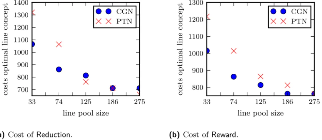
Dependence on the size of the line pool
We have already seen that for larger line pools, cost optimal solutions are obtained by Reduction and for smaller line pools by Reward. Figures 3 and 4 now study further the dependence of the line pool.
In all our experiments, the best travel time was achieved by Shortest Paths. In Figure 3 we see that the travel time is lower if we route in the CGN compared to routing in the PTN for all instances we computed. The difference gets smaller with an increasing size of the line pool; for the complete line pool routing in the CGN and in the PTN would coincide.
For RewardandReductionwe see two effects: First we see a decrease in the costs when we have more lines in the line pool. This is to be expected, since the line concept algorithm used profits from a bigger line pool. Furthermore, we see the forReductionthere are cases, where the cost optimal solution can be found with the PTN routing.
30.0 30.5 31.0 31.5 32.0 travel time
1000 1050 1100 1150 1200 1250
costsoptimallineconcept
end
(a)Iterations forReduction,γ= 75, 186 lines. (b)Solution evaluated by VISUM.
Figure 5
Tracking the iterative solutions in Reduction and Reward
ReductionandRewardare iterative algorithms. They require an assignment in each iteration.
For each of these assignments we can compute a line concept and evaluate it. Such an evaluation is shown in Figure 5a where we depict the line concepts computed for the passengers’
assignments in each iteration forReduction. ForReward, see [9]. ForReductionwe see that the rerouting in the reduced network in the end is crucial. In most of our experiments the resulting routing dominates all assignments in intermediate steps with respect to costs and travel time of the resulting line concepts. ForRewardwe observe no convergence. It may even happen that some of the intermediate assignments lead to non-dominated line concepts.
6.2 Using the line plan as basis for timetabling and vehicle scheduling
In this section we exemplarily evaluate the line concept obtained byReductionwith routing in the PTN for a large line pool of 275 lines in more detail. The line plan is depicted in Figure 5b. For its evaluation we usedLinTim[1, 11] to compute a periodic timetable and a vehicle schedule. The resulting public transport supply was evaluated by VISUM ([16]).
More precisely, we computed
the cost for operating the schedule given by the number of vehicles, the distances driven and the time needed to operate the lines, and
the perceived travel time of the passengers (travel time plus a penalty of five minutes for every transfer) when they choose the best possible routes with respect to the line plan and the timetable.
The resulting costs are 1830 which leads to be best completely automatically generated solution obtained so far for this example (for other solutions, see [8]) and shows that the low costs in line planning lead to a low-cost solution when a timetable and vehicle schedule is added. As expected, the travel time for the passengers increased (by 18%).
7 Conclusion and Outlook
We showed the importance of the traffic assignment for the resulting line concepts, regarding the costs as well as the passengers’ travel time. We analyzed the effect of different assignments theoretically as well as examined three assignment algorithms numerically. As further steps
we plan to analyze the impact of the passengers’ assignment together with the generation of the line pool. We also plan to develop algorithms for solving (LineA) exactly with the goal of finding the cost-optimal assignment in the line planning stage, and finally a lower bound on the costs necessary to transport all passengers in the grid graph example. Furthermore, more optimization in the implementation is necessary to solve the discussed models on instances of a more realistic size.
References
1 S. Albert, J. Pätzold, A. Schiewe, P. Schiewe, and A. Schöbel. LinTim – Integrated Opti- mization in Public Transportation. Homepage. seehttp://lintim.math.uni-goettingen.
de/.
2 R. Borndörfer, M. Grötschel, and M. E. Pfetsch. A column generation approach to line planning in public transport. Transportation Science, 41:123–132, 2007.
3 M. R. Bussieck. Optimal lines in public transport. PhD thesis, Technische Universität Braunschweig, 1998.
4 M. R. Bussieck, P. Kreuzer, and U. T. Zimmermann. Optimal lines for railway systems.
European Journal of Operational Research, 96(1):54–63, 1996.
5 M. T. Claessens. De kost-lijnvoering. Master’s thesis, University of Amsterdam, 1994. (in Dutch).
6 M. T. Claessens, N. M. van Dijk, and P. J. Zwaneveld. Cost optimal allocation of rail passenger lines. European Journal on Operational Research, 110:474–489, 1998.
7 H. Dienst. Linienplanung im spurgeführten Personenverkehr mit Hilfe eines heuristischen Verfahrens. PhD thesis, Technische Universität Braunschweig, 1978. (in German).
8 M. Friedrich, M. Hartl, A. Schiewe, and A. Schöbel. Angebotsplanung im öffentlichen Verkehr – planerische und algorithmische Lösungen. InHeureka’17, 2017.
9 M. Friedrich, M. Hartl, A. Schiewe, and A. Schöbel. Integrating passengers’ assignment in cost-optimal line planning. Technical Report 2017-5, Preprint-Reihe, Institut für Nu- merische und Angewandte Mathematik, Georg-August Universität Göttingen, 2017. URL:
http://num.math.uni-goettingen.de/preprints/files/2017-5.pdf.
10 P. Gattermann, J. Harbering, and A. Schöbel. Line pool generation. Public Transport, 2016. accepted.
11 M. Goerigk, M. Schachtebeck, and A. Schöbel. Evaluating line concepts using travel times and robustness: Simulations with thelintimtoolbox. Public Transport, 5(3), 2013.
12 J. Goossens, C. P. M. van Hoesel, and L. G. Kroon. On solving multi-type railway line planning problems. European Journal of Operational Research, 168(2):403–424, 2006.
13 R. Hüttmann. Planungsmodell zur Entwicklung von Nahverkehrsnetzen liniengebundener Verkehrsmittel, volume 1. Veröffentlichungen des Instituts für Verkehrswirtschaft, Straßen-
wesen und Städtebau der Universität Hannover, 1979.
14 S. Kontogiannis and C. Zaroliagis. Robust line planning through elasticity of frequencies.
Technical report, ARRIVAL project, 2008.
15 S. Kontogiannis and C. Zaroliagis. Robust line planning under unknown incentives and elasticity of frequencies. In Matteo Fischetti and Peter Widmayer, editors,ATMOS 2008 – 8th Workshop on Algorithmic Approaches for Transportation Modeling, Optimization, and Systems, volume 9 of Open Access Series in Informatics (OASIcs), Dagstuhl, Germany, 2008. Schloss Dagstuhl – Leibniz-Zentrum für Informatik. doi:10.4230/OASIcs.ATMOS.
2008.1581.
16 PTV. Visum. http://vision-traffic.ptvgroup.com/de/produkte/ptv-visum/.
17 M. Sahling. Linienplanung im öffentlichen Personennahverkehr. Technical report, Univer- sität Karlsruhe, 1981.
18 A. Schöbel. Line planning in public transportation: models and methods. OR Spectrum, 34(3):491–510, 2012.
19 A. Schöbel and S. Scholl. Line planning with minimal travel time. In 5th Workshop on Algorithmic Methods and Models for Optimization of Railways, number 06901 in Dagstuhl Seminar Proceedings, 2006.
20 A. Schöbel and S. Schwarze. A Game-Theoretic Approach to Line Planning. InATMOS 2006 – 6th Workshop on Algorithmic Methods and Models for Optimization of Railways, September 14, 2006, ETH Zürich, Zurich, Switzerland, Selected Papers, volume 6 ofOpen Access Series in Informatics (OASIcs). Schloss Dagstuhl – Leibniz-Zentrum für Informatik, 2006. doi:10.4230/OASIcs.ATMOS.2006.688.
21 A. Schöbel and S. Schwarze. Finding delay-resistant line concepts using a game-theoretic approach. Netnomics, 14(3):95–117, 2013. doi:10.1007/s11066-013-9080-x.
22 C. Simonis. Optimierung von Omnibuslinien.Berichte stadt–region–land, Institut für Stadt- bauwesen, RWTH Aachen, 1981.
23 H. Sonntag. Linienplanung im öffentlichen Personennahverkehr, pages 430–439. Physica- Verlag HD, 1978.
24 H. Wegel. Fahrplangestaltung für taktbetriebene Nahverkehrsnetze. PhD thesis, TU Braun- schweig, 1974. (in German).
25 P. J. Zwaneveld. Railway Planning – Routing of trains and allocation of passenger lines.
PhD thesis, School of Management, Rotterdam, 1997.
26 P. J. Zwaneveld, M. T. Claessens, and N. M. van Dijk. A new method to determine the cost optimal allocation of passenger lines. In Defence or Attack: Proceedings of 2nd TRAIL Phd Congress 1996, Part 2, Delft/Rotterdam, 1996. TRAIL Research School.
A Algorithms
Algorithm 8:CGN routing version of Algorithm 5.
Input: PTN= (V, E),Wuv for allu, v ∈V Construct the CGN ( ˜V ,E) with˜
de˜=
(de, for drive edges ˜e, whereeis the corr. PTN edge pen, for transfer edges ˜e, where pen is a transfer penalty i := 0
we0:= 0∀e∈E repeat
i = i + 1
forevery u, v∈V withWuv>0 do
Compute a shortest path ˜Puvi fromutov in the CGN, w.r.t.
costi(˜e) =de˜+γ· de˜ max{wi−1e ,1},
where eis the PTN edge corresponding to ˜e.
end
forevery e∈E do Setwie:=P
e∈˜ E˜ ecorr. to ˜e
Pu,v∈V
˜e∈˜eiuv
Wuv
end untilP
e∈E(wei−1−wie)2< or i>max_it;
forevery u, v∈V withWuv>0 do
Compute a shortest pathPuv fromutov in the PTN, w.r.t.
cost(e) =
(de, wei >0
∞, otherwise end
forevery e∈E do Setwe:=P
u,v∈V e∈Puv
Wuv end
Algorithm 9: CGN routing version of Algorithm 6.
Input: PTN= (V, E),Wuv for allu, v∈V Construct the CGN ( ˜V ,E) with˜
d˜e=
(de, for drive edges ˜e, whereeis the corr. PTN edge pen, for transfer edges ˜e, where pen is a transfer penalty i := 0
w0˜e:= 0∀˜e∈E˜ repeat
i = i + 1
wi˜e:=wi−1˜e ∀˜e∈E˜
foreveryu, v ∈V with Wuv>0do
Compute a shortest path ˜Puvi from uto vin the CGN, w.r.t.
costi(˜e) = max{de˜·
1−γ· wei−1˜ mod Cap Cap
,0}
forevery ˜e∈P˜uvi−1 do Setwei˜:=wi˜e−Wuv end
foreverye˜∈P˜uvi do Setwei˜:=wi˜e+Wuv end
end
foreverye∈E do Setwe:=P
e∈˜ E:˜
˜
ecorr. toe
Pu,v∈V: e∈˜ P˜uv
Wuv
end untilP
e∈E(wi−1e −wie)2< or i>max_it;