The Chemical Basis of Morphogenesis

(1)

The Chemical Basis of Morphogenesis

A.M.Turing, 1952

The paper discussed is by Alan Turing. It was published in 1952 and presents an idea of how periodic patterns could be formed in nature.

Looking on periodic structures – like the stripes on tigers, the dots on leopards or the whirly leaves on woodruff – it is hard to imagine those patterns are formated by pure chance. On the other hand, thinking of the unbelievable multitude of possible realizations, the patterns can not all be exactly encoded in the genes.

The paper “The Chemical Basis of Morphogenesis” proposes a possible mechanism due to an interaction of two

“morphogenes” which react and diffuse through the tissue. Fulfilling some constrains regarding the diffusibilities and the behaviour of the reactions, this mechanism – calledTuring mechanism– can lead to a pattern of concentrations defining the structure we see.

I. TURING MECHANISM

The central roll is played by two “morphogenes”. This term describes their function as a “form producer”. Morphogenes are not by them self the material that formates the pattern.

They are for example enzymes and their concentrations influence the processes which are creating the pattern e.g. by stimulating or suppressing the production of pigments.

The idea thatdiffusionis a driving force for theformationof patterns might not be that intuitive. In most cases, diffusion destroys patterns of concentration over time.

A picturesque example for pattern formation due to diffusion is the following: Consider random fire outbreaks in a dry forest. The expanding wildfires would then be one morphogene slowly diffusing. A second morphogene in the form of fire fighters diffusesmuch faster(e.g via airplanes) to the seats of fire and extinguishes it. An areal image of the forest would show a green area with a pattern of black patches.

The keys in this example are that:

1. One morphogene is excitatory, the other one is inhibitory.

2. The inhibitory morphogene diffuses faster the excitatory.

A. The Setting

The system of interest is for example an embryo in the early stage of the embryogenesis. The follwing setting will be used:

There are two morphogenes whose concentrations are denoted c₁andc₂, they depend each on the two dimensional positionx and the timet:c_1,2=c_1,2(x,t). Those concentrations underlay in general the influence of the reactions f andg, respectively, and diffusion. The reactions depend on both concentrations each, so: f = f(c₁,c₂)andg=g(c₁,c₂). These functions can take positive and negative values, describing the creation and dismantling of morphogenes. The diffusion is described according to the usual diffusion function byD1∇²c1and analogue for the second morphogene. Altogether, the change over time is described as it follows:

˙

c1=f(c₁,c2) +D1∇²c1

˙

c₂=g(c₁,c₂) +D₂∇²c₂

what is known as aReaction-Diffusion System.

A slightly different and less intuitive notation will be used:

˙

u=γf(u,v) +∇²u

˙

v=γg(u,v) +d∇²v, (1) what is justified by making the calculations later more natural.

In Eq. (1),c₁is rescaled tou andc₂tov. γ =L²/D₁T rep- resents the scaling factor withLthe spatial,T the time scale.

The diffusibilities are normalized with respect toD1and so the second equation get assigned the factord=D₂/D₁.

B. Turing Mechanism

Obviously there is a multitude of solutions for this differen- tial equations Eq. (1). But to be aTuring mechanismthere are three conditions that must hold:

(I) There is a homogeneous and stationary positive solution (u₀,v0)for f(u₀,v0) =g(u₀,v0) =0.

(II) The System is stable ifnodiffusion occurs.

(III) The System is unstable under diffusion.

These constraints limit the space of solutions to those describing systems where diffusion driven pattern formation is possible.

II. TURING ANALYSIS

The three conditions implicate constraints for both the reactions and the diffusion, which will be shown here. The process of checking for the above claims to hold is calledTuring analysis.

a. First Condition To check if a homogeneous and stationary positive solution exists, determine the solution for f(u₀,v₀) =g(u₀,v₀) =0. The existence of such a solution means that there is a pair ofc₁,c₂ for which both reactions neither produce, nor destroy either of the morphogenes. Since negative concentration make no sense, the solution must be positive.

(2)

2 b. Second Condition The second condition requires,

that the system has to be stable if the diffusion is suppressed The Reaction-Diffusion system Eq. (1) therefore misses the diffusion term, and reads:

˙

u=γf(u,v)

˙

v=γg(u,v).

This should be stable under a small perturbation around the stable state(u₀,v₀), which is the solution from the first condition.

The perturbed stable states are written as w=

u−u0

v−v0

.

As the system can be considered as linear,wbehaves likew∝ e^λt.

With the shorthand f_u=∂f/∂uthe Jacobian matrix reads:

A= f_u f_v

g_u g_v

.

It follows, that at the stable state(u₀,v₀)the linear behaviour yields:

˙ w=γAw.

Since the System has to be stable under this perturbation for the condition to hold, the eigenvalues λ1,2 solving det(γA− λ1) =0 have to be negative.

The eigenvalues are given by:

λ1,2=1 2γ

(f_u+g_v)± q

(f_u+g_v)²−4(f_ug_v−f_vg_u)

. (2)

For the real part of λ1,2 to be negative, the term in front of the square root must be negative and the last one in the square root positive. So the requirement of the state to be stable with no diffusion present implies conditions on the derivatives of the functions describing the reactions:

fu+gv<0 (3) f_ug_v−f_vg_u>0. (4) Thus this condition gives constraints to how the behaviour of the reactions change with respect to a change in the concentrations.

c. Third Condition The last condition demands, that the system becomes unstable, as the diffusion is again considered.

For this the diffusion term from Eq. (1) has to be taken into account. In the now used notation and with the diffusion, lin- earized dynamics reads:

˙

w=γAw+D∇²w, (5)

with the matrixDcontaining the information about the diffusibilities:

D= 1 0

0 ^D_D²

1

.

As discussed before, the concentrations depend on both, space and time, hencew=w(x,t). A separation ansatz is used to disentangle the two dependencies:

w(x,t) =

∑

k

c_ke^λ^k^tW_k(x). (6) The respective state of the two concentrations at the location xand the timetis expressed as a series of modes. Each mode kseparates in a spacial eigenfunctionW(x)and the “time de- velopment”e^λ^k^tof the starting statec_k.

Still considering linear behaviour ofw(x,t)under a small perturbation, Eq. (5) yields for a modek

λ(k)W_k=γAW_k+D∇²W_k. (7) This expression describes thek’th mode (withkis the wave number k∝1/λ), note that the notation is not perfectly

“clean” in a mathematical sense, sincekis used ambiguous as a index and a parameter. This is justified by its physical meaning.

In order to get rid of the second derivative in the diffusion term, the solution of the spacial eigenvalue problem is used:

∇²W(x) +k²W(x) =0.

This allows to replace∇²by−k²in Eq. (7):

λ(k)W_k=γAW_k+D∇²W_k

=γAW_k−Dk²W_k.

Since the system should be unstable now, the resulting real parts of the eigenvalues λ1,2 from det(λ1−γA+Dk²) =0 must be positive. The eigenvalue equation reads:

0=λ²+λ

k²(1+d)−γ(f_u+g_v)

+h(k²).

With the last term short for

h(k²) =dk⁴−γ(d f_u+g_v)k²+γ|A|.

The system is unstable whenRe(λ(k))>0, that means that either:

• [k²(1+d)−γ(f_u+g_v)]<0

• h(k²)<0

The first expression can not be true, since the diffusion must be positive and therefored>0, and f_u+g_v<0 is a result from Eq. (3).

Thus, for the system to be unstable it must hold that h(k²) =dk⁴−γ(d f_u+gv)k²+γ|A|<0. (8) Because all other values contribute positive, forh(k²)<0 it must hold that(d f_u+g_v)>0.

So, at the same time it has to hold, that(d f_u+g_v)>0 and (f_u+g_v)<0 (known from Eq. (3)). That leads to some im- plications:

(3)

3

• f_uandg_vhave different signs. The morphogeneutypi- cally acts autocatalytic, therefore f_u>0,g_v>0.

• The sum changes the sign asd is applied to f_u. That means, thatD₂/D₁>1. So the inhibitory morphogene diffuses faster than the excitatory, which was used in the illustration above.

While being a necessary criterion,(d f_u+gv)>0 by itself is not sufficient. For the third condition to hold true in total, Eq.

(8) must be fulfilled. For thish(k²)(andk², respectively) is evaluated at the minimum:

hmin=γ²

|A| −(d f_u+g_v)² 4d

, k²_min=γ(d f_u+g_v)

2d (9)

it holds, thath(k²)<0 for:

(d f_u+g_v)²

4d >|A|. (10)

III. PATTERN FORMATION

If all the constraints to the space of possible solutions are fulfilled, it is possible for a pattern to be formed. That means there is a critical valued_c for which smaller values do not fulfill the third condition:

|A|=(d_cf_u+g_v)² 4d_c .

The meaning of this can be made clear by once again using the image from above. For a wildfire resulting in a pattern of burned forest the difference in the diffusibilities is a key. If the firefighters are too fast, the fire would not have the necessary time to burn a patch down. If they are too slow, all the forest would have burned down, and again no pattern would appear in the end.

In this model, with Eq. (9), the existence of ad_cimplies, that there is ak_cfor that:

k²_c=γd_cf_u+g_v 2d_c =γ

s

|A|

dc

.

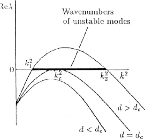
Depending on the value ford, there is a singlek(in this case:

k=k_c), a range ofkvalues or nok, for that patterns are possible:

• Ford>d_c: roots atk₁,k₂, instable fork∈[k₁,k₂]

• Ford=d_c: root atk_c, instable fork_c

• k∈/[k₁,k₂]: nokvalue to fulfil the third condition, therefore no pattern.

As shown in Fig. 1, any case there are some small and largek, for that no patterns are possible.

FIG. 1. Visualization of the range ofkfor which patterns can occur.

source: J.D. Murray, Mathematical Biology II: Spatial Models and Biomedical Applications

An example for no pattern for largekwould be a carpet for that black and white yarn alternate in so narrow distances, that it appears grey. Analogue, if the frequency is too low (small k) there would not be any change of color at all.

All in all, the three conditions lead to constraints to the forms of f(u,v)andg(u,v):

The need for stability while suppressing the diffusion gives:

f_u+g_v<0 f_ug_v−f_vg_u>0.

While the instability under spatial perturbation yields:

d f_u+g_v>0 (d f_u+g_v)²>4d|A|.

A. Visualisation

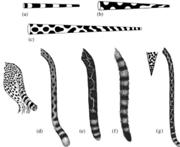
The impact of the spacial aspect on the pattern formation can be shown by simulating different sizes by changing the scale parameterγin Eq. (1):

FIG. 2. Simulation of different fur sizes.

As seen in Fig. 2 this mechanism does not lead to pattern formation for both cases of very small (e.g. a mouse) or very

(4)

4 large (elephant for example) fur sizes. This prediction is ful-

filled by the majority of animals with the respective size. It has to be noted tho, that the here discussed mechanism of pattern formation is not the only one in nature (but the only diffusion driven). The reason why there are no pattern for too small fur sizes is straight forward. The spacial constraint re- stricts the possible wave modes to a region close tok=0 and so suppresses pattern formation. As the size gets bigger pattern begin to appear. First with low frequency as seen in goats and sheeps for example, than more complex like on chetha, leopards and so on. The upper end of the scale appears again unicolored. The reason here is, that the frequency is to high and the dominant wave modes tend tok→∞.

There are some comparisons between the simulation and real patterns. For example in Fig. 3 for different species of giraffe:

FIG. 3. Comparison between simulated (right) and real (left and mid- dle) patterns of different giraffe species.

An interesting effect can be seen at Fig. 4. Thinking of the fur as a two dimensional surface, the dots on chethas represent the overlap of weaves in different dimensions. The tail can then be seen as effective reduction to one dimension. If thex axis is defined along the tail, the expansion inyunderlays the same condition and effect as for small fur sizes in general, but the suppression of pattern only effects one dimension, so the dots transform to stripes.

This is the reason, why spotted animals can have striped tails but not vice versa. The latter would imply, that in the tail waves from the ydirection appear that are not there in the main area of the fur.

FIG. 4. Comparison between simulated (above) and real (below) tails of different chetha species.

IV. SUMMARY

In the early stages of the embryogenesis, the embryo can be considered as homogeneous tissue. In this phase the reaction and diffusion does not depend on the spatial parameter. The mechanism of pattern formation proposed by Alan Turing describes a set of conditions, under which pattern can be formed in this stage. The whole process bases of the assumption of linear behaviour under small perturbations in the spacial distribution of the concentrations, like they are usual due to ther- mal influences for example. In the limit of large times, this assumption will lose its legitimacy eventually. At this point in the embryogenesis the process will ultimately halt. The cur- rent distribution of concentration will be “frozen” so to say.

Since the concentrations are those of morphogenes there will be a visual pattern following the pattern of concentrations.

This process gives an elegant possibility of how the unbelievable diversity of different expressions can be coded. The specific morphogenes in action with their specific diffusibilities and reactions determine the length scale The concrete expression however is exposed to random effects.

V. LITERATUR

1A. M. TURING, “The Chemical Basis of Morphogenesis”. University of Manchester, August 1952

2J.D. MURRAY, “Mathematical Biology II: Spatial Models and Biomedical Applications”. Springer, 2011

3J.TIMMER,“Dynamische Modelle in der Biology; Von der Mathematischen Biologie zur Systembiologie”Script, University Freiburg, 2016