September 2020
Computational Finance
Modeling, numerics, applications
Lecture Notes
Univ.-Prof. Dr. Ansgar J¨ ungel
Institut f¨ ur Analysis und Scientific Computing
This manuscript is mainly based on the following book: Finanzderivate mit MATLABof M. G ¨un- ther and A. J ¨ungel. Further main sources are the books of R. Seydel,Tools for Computational Fi- nance, P. Kloeden and E. Platen,Numerical Solution of Stochastic Differential Equations, and G. Lord, C. Powell, and T. Shardlow,An Introduction to Computational Stochastic PDEs.
Contents
1 Introduction 4
2 Basics 10
2.1 Financial options . . . 10
2.2 Stochastic analysis . . . 14
3 The Black-Scholes model 25 3.1 Black-Scholes formulas . . . 25
3.2 Risk-neutral valuation . . . 33
3.3 Implied volatility . . . 36
3.4 Options on dividend paying assets . . . 38
3.5 Multi-asset options . . . 42
3.6 Stochastic interest rate and volatility . . . 44
3.7 Application: Pricing Asian options . . . 47
3.8 Beyond Black-Scholes . . . 49
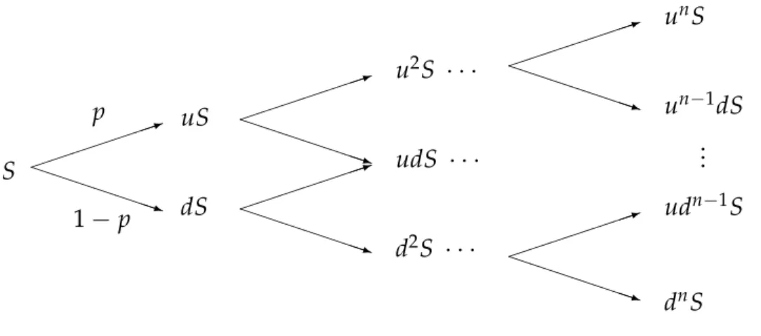
4 Binomial models 58 4.1 The Cox-Ross-Rubinstein model . . . 58
4.2 Relation with the Black-Scholes formula . . . 61
4.3 Binomial method . . . 63
5 Monte-Carlo method 67 5.1 Pseudo random numbers . . . 68
5.2 Euler-Maruyama method . . . 72
5.3 Milstein method . . . 78
5.4 It ˆo-Taylor and Runge-Kutta schemes . . . 81
5.5 Systems of stochastic differential equations . . . 86
5.6 Quasi Monte-Carlo method and variance reduction . . . 88
5.7 Multilevel Monte-Carlo method . . . 94
5.8 Application: Pricing Asian options in the Heston model . . . 95
6 Finite-difference methods 98 6.1 Theθ-method . . . 98
6.2 Application: Pricing arithmetic-average floating-strike calls . . . 106
6.3 Relation with the binomial method . . . 108
6.4 Pricing American options . . . 110
6.5 Application: Pricing swing options in electricity markets . . . 118
References 122
CONTENTS 3
English German
compound interest Zinseszins
expiry date/maturity Verfallstag/F¨alligkeit
fixed-term deposit Festgeld
holder K¨aufer einer Option
interest Zins
interest rate Zinssatz
loan Kredit
payoff Auszahlung
premium Optionspreis
savings account Sparguthaben
share Anteil
stock Aktie
strike/exercise price Aus ¨ubungspreis
time to expiration Laufzeit
underlying (asset) Basiswert
volatility Preisschwankung/Volatilit¨at
writer Verk¨aufer einer Option
Table 1:English-German translations of financial terms used in the lecture notes.
1 Introduction
A financial derivative is an agreement between two parties based on an underlying asset (or just underlying). It is designed to hedge financial transactions, but they can be also used to speculate on the prices of the underlying. Already in ancient Greece, shipping contracts for trading were used, similar to forward contracts (see below). The buyer receives some money upfront, which finances the trading voyage. After return (if successful), the buyer pays back the loan and the required interest. Similar commodity forward contracts were used in the Roman era, in Italy from the 10th century on, and in Japan in the 18th century.
In the 17th century, financial options were issued to hedge the rapidly increasing prices of tulip bulbs, which were very fashionable at that time. In these options, the obligation to purchase tulip bulbs at a fixed price was converted to an opportunity to do so. The tulip market was accompanied by wild speculative transactions, leading eventually in February 1637 to a collapse of the tulip bulb contract prices.
Later, further precursors of today’s financial derivatives have been issued and traded, but a regulated market was still missing. In 1848, the Chicago Board of Trade opened, providing a central location as a storage and market place for grain. Some years later, in 1865, the contracts were standardized. The Chicago Board Option Exchange, founded in 1973 as an extension of the Chicago Board of Trade, then became the first exchange to offer standardized options trading.
Derivatives gained widespread use in the 1970s, fostered by the computer technol- ogy allowing the complex models and computations to be solved in an efficient way.
In the same decade, in 1973, Fischer Black and Myron Scholes published their seminal paper “The pricing of options and corporate liabilities”. Robert Merton expanded the mathematical understanding of the option pricing model. (Interestingly, Louis Bache- lier already formulated in 1900 a theory of option pricing in his PhD thesis, far before Black, Scholes, and Merton. However, Bachelier did not include a theory of hedging and replication by dynamic strategies; see the discussion in [32].) The Black-Scholes formula led to a boom in option trading. Merton and Scholes received the Nobel Memorial Prize in Economic Sciences in 1997 for their new methodology to value derivatives (Black died in 1995 and could not receive the award). Nowadays, in spite of the financial crisis from 2007, the derivative market is huge – its size is estimated to be more than ten times larger than the total world gross domestic market. Therefore, the understanding and control of financial instruments is of paramount importance for companies and also for the society.
These lecture notes are devoted to the modeling and numerical simulation of financial derivatives. In particular, we derive the Black-Scholes equation and the Black-Scholes formula, discuss its limitations and extensions, and present some numerical techniques to solve the corresponding financial models. The topic forces us to use several mathe-
5
matical techniques:
◮ mathematical modeling,
◮ stochastic analysis,
◮ theory of partial differential equations,
◮ numerical analysis.
The lecture notes are organized in such a way that no special knowledge is assumed to follow the arguments – besides of calculus, ordinary differential equations, and a basic understanding of probability theory.
What is a financial derivative? It is a contract whose value at the expiry date is de- termined by the value of the underlying asset at or up to expiration. The underlying asset can be, for instance, a stock, commodity, index, or currency. Generally, we can distinguish four classes of financial derivatives:
◮ Forward contracts.A forward contract is an agreement between two counterparties to sell or purchase an asset for a price agreed upon today with delivery and pay- ment at a fixed future date. Forwards can be used to hedge risks like currency rate risk.
◮ Future contract. Future contracts are very similar to forward contracts. They are standardized contracts between two counterparties to sell or purchase an asset for a price agreed upon today with delivery and payment at a fixed future date. In contrast to forwards, they are exchange-traded and both parties are required to put up an initial amount of cash to mitigate the risk of default of either party.
◮ Option contracts. Option contracts give the owner the right, but not the obligation, to sell or purchase an asset for the exercise price until or at the expiry date. In contrast to forward or future contracts, the owner has no obligation to carry out the right of selling or buying the underlying asset. This allows the owner to hedge or mitigate risk due to changes in the asset price.
◮ Swaps. A swap is a contract determining the cash flow exchange of the counter- parties. For instance, one party may exchange an uncertain cash flow to a certain one or to swap a fixed interest rate to a floating one. Swaps are used to hedge risks like the interest rate or currency risk, but they may be also used to speculate on changes of the underlying price. Common swaps are interest rate swaps, currency swaps, credit swaps, commodity swaps, and equity swaps.
We see that financial derivatives are defined through the following values:
◮ the quantity and class of the underlying asset,
◮ the expiry date,
◮ the excercise or strike price,
◮ the type of contract (the right or obligation to buy or sell the asset).
In the lecture notes, we focus on financial options. The most common ones arevanilla
options, and we distinguish betweenEuropean andAmerican options. The former option class can be exercised only at the expiry date, the latter one can be exercised until or at expiration. Each of these two option classes can be exercised as acall optionorput option.
The holder of a call option has the right to buy a fixed amount of the underlying for a fixed price from the option seller (called the writer), while a put option gives the holder the right to sell a fixed amount of the underlying for a fixed price to the writer; see Table 2. A more formal definition of European options is as follows.
Call Put
European Exercise at expiry only Exercise at expiry only Right to buy the underlying Right to sell the underlying American Exercise until or at expiry Exercise until or at expiry
Right to buy the underlying Right to sell the underlying Table 2: Overview of vanilla options.
Definition 1.1 (European option). AEuropean call (put) optionis a contract with the following conditions: The holder of the option has the right but not the obligation to buy the underlying from the writer (to sell the underlying to the writer) at the expiry date T for the fixed strike or exercise price K.
The option gives a right, so it has a value. We denote the value of an call option at time tbyCt = C(t), the value of a put option byPt = P(t).1 Let St be the value of the underlying at timet. At expiration, we may distinguish two cases for a call option:
◮ ST > K: We exercise the option, purchase the underlying at price K, and sell it immediately on the spot for the priceST. We realize the profitST−K >0.
◮ ST <K: The right to exercise the option is not interesting since we can buy the un- derlying on the market for a cheaper price than guaranteed by the option contract.
The option expires.
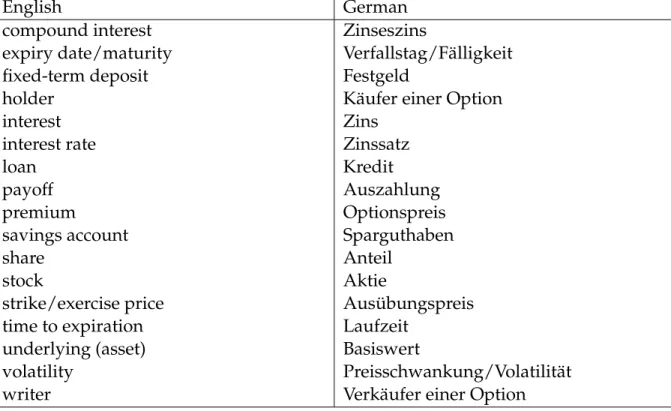
This shows that the valueCT of the call option at expiration (the so-calledpayoff) is CT =max{0,ST−K}= (ST −K)+.
We can use similar arguments to determine the payoff of a put option. IfST >K, the put option has no value since we can sell the underlying for a higher price on the market, while for ST < K, we buy the underlying on the spot for the price ST, exercise the
1It is common in the theory of stochastic processes to use an index for the time variable. The notation C(ω)or P(ω)is used for the stochastic variablesω. In the theory of partial differential equations, an index usually means partial differentiation with respect to that variable. We try to avoid any confusion, which may arise because of these two conventions.
7
option, and sell the underlying for the priceK. We realize the profitK−ST >0. Thus, the payoff PT of the put option equals
PT = (K−ST)+.
The holder of a call option bets on rising prices, while the writer speculates on falling prices. The opposite holds for put options. The payoff of European options can be illustrated by thepayoff diagramsin Figure 1.1.
✻
✲
CT
K S 0
PT ✻
K S K
0
❅❅
❅❅
❅❅ ✲
Figure 1.1:Payoff diagrams of a European call option (left) and put option (right).
Remark. (1) Our arguments only hold when we neglect transaction costs, bid-ask spreads, etc. We specify these assumptions in section 3.1 and discuss models including transaction costs in section 3.8.
(2) When an option is exercised, usually the underlying will not be delivered physically but just the profit will be paid out (this is calledcash settlement). As we already mentioned, options may be used tospeculateon falling or rising prices or tohedgethe underlying asset against price fluctuations and to mitigate risk.
We denote the value of a (call or put) option by V(S,t). This means that V is a function of time tandall possible realizationsof the value of the underlying S, modeled by a function St(ω) := S(ω,t), where the stochastic variable ω varies in the set of all possible events. At time t, exactly one value of the underlying St is realized, and the value of the option is V(St,t), but the function V is defined for all values S. The key question is: Which is the “fair” price V(S, 0) at time t = 0, when the writer sells the option?
We will show below that, under some assumptions on the financial market, the fair priceV(S,t)satisfies the following partial differential equation, the Black-Scholes equa- tion:
∂V
∂t +1
2σ2S2∂2V
∂S2 +rS∂V
∂S −rV =0, S∈ (0,∞), t ∈ (0,T).
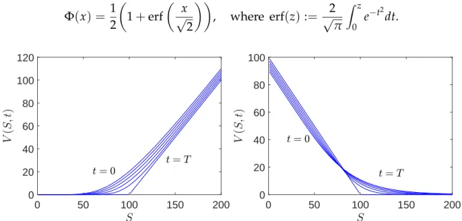
Here, the parameterr ≥0 is the riskfree interest rate andσ >0 the volatility, a measure for the fluctuations of the underlying. At timet =T, the value of the option is known:
V(S,T) =
(S−K)+ : call (K−S)+ : put.
Boundary conditions at S = 0 and S → ∞ will be specified in section 3.1. Thus, the differential equation has to be solved backwards in time, and we are looking for the solution V(S,t) at t = 0. Interestingly, the equation can be transformed to the heat equation and solved explicitly, leading to the Black-Scholes formula. The Black-Scholes theory will be detailed in section 3.
In contrast to European options, American options can be exercised at or before the expiration date. The formal definition is as follows.
Definition 1.2 (American option). AnAmerican call (put) optionis a contract with the following conditions: The holder of the option has the right but not the obligation to purchase the underlying from the writer (to sell the underlying to the writer) at any time before and including the expiry date.
The value of an American call or put option at time t= Tis the same as for the cor- responding European option. Since American options can be also exercised before the expiration date, its value is at least as large as the value of the corresponding European option. Besides the value of the American option at timet = 0, we also need to deter- mine the optimal exercise date. This leads to a free-boundary problem. We will study American options in section 6.
Exotic options are all options which are not of vanilla style (European or American options). We mention some of them:
◮ TheBermudan optioncan only exercised on specified dates on or before expiration.
The American option is a special case of a Bermudean option.
◮ The payoff of an Asian option is determined by the average of the price of the underlying over some time period.
◮ Thebarrier optionrequires that the price of the underlying must or must not pass a certain level or barrier before it can be exercised.
◮ The binary option pays a certain amount if the price of the underlying satisfies some defined condition on expiration. Otherwise, it expires. Therefore, is is an all-or-nothing option.
◮ The payoff oflookback optionsdepends on the minimum or maximum of the price of the underlying.
◮ Multi-asset optionsdepend on several underlyings, and correspondingly, the payoff depends on the price of these underlyings at expiration.
While the value of European options can be determined explicity under some con- ditions on the market, this does not hold true in more general situations or for certain exotic options. This makes it necessary to develop numerical methods to determine approximate values for the option price. In these lecture notes, we will discuss three numerical techniques:
◮ Binomial methods (section 4),
9
◮ Monte-Carlo methods (section 5),
◮ finite-difference methods (section 6).
In section 2, we investigate basic properties of vanilla options and basic elements of stochastic analysis, needed for the derivation and formulation of the Black-Scholes equations presented in section 3.
2 Basics
2.1 Financial options
The price of a European option can be determined explicitly under some simplifying assumptions on the financial market. The most important condition is the absence of arbitrage. Arbitrage is the riskfree profit by exploiting a price difference between two markets or two financial products. To illustrate this notion, let us consider a simple example taken from [16, Beispiel 1.3].
Example 2.1 (Arbitrage). We consider a financial market that allows for only three investment possibilities: a bond, a stock, and a European call option. The bond is a debt security which requires the writer to pay interest (called the coupon) to the holder and to pay the principal at a fixed later date, similar to a fixed-term deposit.
We neglect default risk and assume that the bond is riskfree. The values of the bond, stock, and option at time t are denoted by Bt, St, and Ct, respectively. We assume that at time t = 0, B0 = 100, S0 = 100, and C0 = 10. The call option has the strike priceK =100 and the expiration date T. We assume that trading is only possible at t = 0 andt = Tand that there exist only two states of the financial market, “high”
and “low” with
“high”: BT =110, ST =120,
“low”: BT =110, ST =80.
We construct the following portfolio: We buy 2/5 shares of the bond and one call option and sell 1/2 share of the stock. The portfolio at time t = 0 becomes π0 =
2
5·100+10−12·100=0, i.e., initially it has no value. At timet =T, we have
“high”: πT = 2
5·110+ (120−100)+−1
2·120=4,
“low”: πT = 2
5·110+ (80−100)+−1
2·80=4.
Thus, the portfolio has always the value 4 at time t = T. Then the portfolio must have a positive value also at timet =0, and the holder could sell it at time t =0 to realize an instantaneous riskfree profit. This is called arbitrage.
Why do we have arbitrage? The reason is that the price for the call option is too low. If any investment has the same chances of profit, there are numbers c1,c2 ∈ R such that
c1·Bt+c2·St =Ct fort=0,T.
2.1 Financial options 11 Clearly, the fair price att=0 isC0=c1·B0+c2·S0. At timet=T, we have
“high”: c1·110+c2·120= (120−100)+ =20,
“low”: c1·110+c2·80= (80−100)+ =0.
This is a linear system with solutionc1=−4/11 andc2 =1/2. We infer that C0 =− 4
11·100+1
2 ·100 = 300
22 ≈13.64.
As we have replicated the call option by means of the bond and stock, this approach is called areplication strategy.
The assumption of the absence of an instantaneous and riskfree profit (arbitrage) is fundamental in the theory of financial markets. A savings account is generally riskfree but the interest is paid only after some time; options may allow for an instantaneous profit but the investment if not riskfree. Real markets are not free of arbitrage. We assume that the financial market is efficient (liquid, accessible, and transparent) which rules out arbitrage opportunities. Interestingly, we can determine some bounds on the option prices just from the assumption of absence of arbitrage.
To derive these bounds, we consider a financial market with the following assump- tions:
◮ there is no arbitrage,
◮ there are no dividend payments on the underlying,
◮ the riskfree interest rate is the same for investments and loans,
◮ the market is liquid and accessible (i.e., trading is possible at any time).
The riskfree interest rate is denoted byr ≥0, and we suppose continuous interest pay- ments. This means that the return of an investment K0 > 0 after time t = T equals K =K0erT. This formula can be derived from discrete returns att =△t, . . . ,n△t, where n△t=T. Including compound interest, the return equals afternpayments:
Kn =K0(1+r△t)n =K0(1+rT/n)n →K0erT asn→ ∞.
If we invest today the amountKe−rT (or buy a bond with valueKe−rT), we receive the valueKafter time T. The factore−rT is called thediscount factor.
We claim the following relationship between bond, option, and stock value.
Proposition 2.2 (Put-call parity). Under the stated assumptions on the financial market, it holds that
St +Pt−Ct =Ke−r(T−t) for all0≤t≤T, where Pt :=P(St,t)and Ct :=C(St,t).
Proof. Consider the following portfolio: Purchase a stockSand a European put option
Pwith strikeKand expiryTand sell a European call option with strikeKand expiryT.
The portfolio has the valueπ =S+P−C. At timet=T, its value is πT =ST + (K−ST)+−(ST−K)+ =K.
We claim that the value equals πt = Ke−r(T−t) for any t < T. This corresponds to a bond with valueKe−r(T−t) at timet.
Suppose thatπt < Ke−r(T−t) at some timet. Then we buy the portfolio, borrow the amountKe−r(T−t)and put asideKe−r(T−t)−πt >0. At timet=T, the portfolio has the valueKwhich we use to pay back the loan. This means that we have realized at timet the instantaneous riskfree profitKe−r(T−t)−πt >0; contradiction.
Suppose that πt > Ke−r(T−t) at some time t. Now, we sell the portfolio, invest Ke−r(T−t) in a riskfree bond and put aside πt −Ke−r(T−t) > 0. At time t = T, we sell the bond which has the value K and buy back the portfolio. We have realized an
instantaneous riskfree profit; contradiction.
European options satisfy the following bounds.
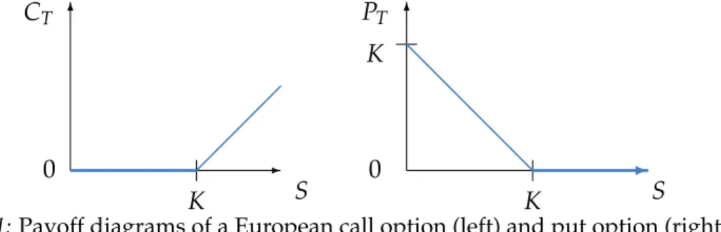
Proposition 2.3 (Bounds for European options). It holds for0≤t≤ T that (i) (St −Ke−r(T−t))+ ≤Ct ≤St,
(ii) (Ke−r(T−t)−St)+ ≤Pt ≤Ke−r(T−t).
Proof. We only consider the call option. The bounds for the put option follow from those for the call option and the put-call parity.
The lower bound Ct ≥ 0 is clear since otherwise, a call with Ct < 0 would yield an instantaneous riskfree profit. It holdsCt ≤ St since otherwise, we sell the call and purchase the underlying. At timet =T, we maybe need to sell the underlying to fulfill the obligation of the call contract. Still, because of Ct −St > 0, we have realized an instantaneous riskfree profit at timet, which is a contradiction.
To show the remaining bound Ct ≥ St −Ke−r(T−t) for all t, we assume that Ct <
St −Ke−r(T−t) for some t. We sell the underlying, buy the call, and invest riskfree the amount Ke−r(T−t). The portfolio is πt = Ct −St +Ke−r(T−t) < 0 but we possess the amount−Ct+St−Ke−r(T−t) >0. At timeT, there are two possibilities:
◮ IfST ≤KthenπT =0−ST+K ≥0.
◮ IfST >KthenπT = (ST−K)−ST+K =0.
We realize the profit−Ct+St−Ke−r(T−t) >0; contradiction.
Similar bounds can be shown for American options with values CA, PA. The values of the corresponding European options are denoted byCE. PE.
2.1 Financial options 13
Proposition 2.4 (Bounds for American options). It holds for0≤t≤ T:
(i) (St−Ke−r(T−t))+ ≤CA(St,t) ≤St, (ii) CA(St,t) =CE(St,t),
(iii) Ke−r(T−t) ≤St+PA(St,t)−CA(St,t) ≤K, (iv) (Ke−r(T−t)−St)+ ≤ PA(St,t) ≤K.
In real markets, the value of American and European call options is generally not the same because of dividend payments. Statement (iii) can be seen as a put-call parity for American options.
Proof. (i) This follows as in the proof of Proposition 2.3.
(ii) Assume that we exercise the American option at time t < T. We receive the amountSt−K >0 (ifSt−K≤0, we would not exercise the option). It follows from (i) that
CA(St,t) ≥(St−Ke−r(T−t))+ =St−Ke−r(T−t) >St−K.
This means that it is better to sell the option than to exercise it. Thus, the early exercise it not optimal, but then the option works like a European option.
(iii) Since American put options are more flexible than European ones, we havePA ≥ PE. By the put-call parity and (ii), we infer that
CA−PA ≤CE−PE =St−Ke−r(T−t),
which is the lower bound. For the upper bound, we apply an arbitrage argument.
Assume that St −K > CA(St,t)−PA(St,t) for some t. Consider the portfolio πt = CA(St,t)−PA(St,t)−St +K < 0. The cash flow gives −πt > 0. Let τ ≤ T be the exercise time of the American put option. It holds that τ ≥ t since otherwise, the put option has already been exercised before timet. We distinguish two cases:
◮ IfSτ ≤Kthen (because ofCA ≥0)
πτ =CA(Sτ,τ)−(K−Sτ)−Sτ+Ker(τ−t) ≥ −K+Ker(τ−t) ≥0.
◮ IfSτ >Kthen (because ofCA(Sτ,τ) ≥Sτ−K >0)
πτ ≥(Sτ−K)−0−Sτ+Ker(τ−t) =−K+Ker(τ−t) ≥0.
We have found a portfolio that allows for arbitrage; contradiction.
(iv) The inequalities in (iii) can be formulated as
Ke−r(T−t)−St +CA≤ PA ≤K−St+CA.
Now, we know from (i), (iii), and Proposition 2.3 (i) that
PA ≥Ke−r(T−t) −St+CE ≥Ke−r(T−t)−St+ (St−Ke−r(T−t))+
= (Ke−r(T−t)−St)+,
PA ≤K−St+CE ≤K−St+St =K.
This ends the proof.
Remark. The lower bound for American put options can be strengthened to PA(St,t)≥(K−St)+.
Indeed, the case K ≤ St means that PA ≥ 0 which is trivial. Therefore, let K > St. If PA(St,t)<(K−St)+=K−Stfor somet, we buy a put option and excercise it immediately to make the riskfree, instantaneous profit(K−St)−PA(St,t)>0; contradiction.
The bounds for European and American option values are illustrated in Figure 2.1.
✻
✲
St Ke−r(T−t)
PA(t) K
PE(t)
K
✻
✲
St Ke−r(T−t)
❅❅
❅❅
CA(t) =CE(t)
Figure 2.1:Qualitative illustration of the prices of European and American options. It is assumed that there are no dividend payments.
2.2 Stochastic analysis
We give a concise introduction to basic elements of stochastic analysis, which are needed to formulate the stochastic asset price dynamics and to valuate financial options. We only state the needed results and refer for proofs and examples to the literature, for instance, [3, 10, 27].
The key object are stochastic processes [27, Section 2]. For this, let Ω be an arbi- trary set (the set of all possible events). A σ-algebra F onΩis a family of subsets of Ω satisfying the following properties:
(i)∅ ∈ F, (ii)∀A ∈ F : Ω\A∈ F, (iii)∀An ∈ F : [∞
n=1
An ∈ F.
2.2 Stochastic analysis 15
For instance, the collection of open sets on a topological space forms a σ-algebra, the Borelσ-algebra. Aprobability measureP :F → [0, 1]is a function satisfying
(i)P(∅) =0, P(Ω) = 1,
(ii) ∀An ∈ F pairwise disjoint : P [∞
n=1
An
=
∞
∑
n=1
P(An). We call the triple(Ω,F, P)aprobability space.
Let X : Ω → R be any function on (Ω,F, P). We call this function F-measurable if X−1(U) = {ω ∈ Ω : X(ω) ∈ U} ∈ F for all open (or all Borel) sets U ⊂ R. A random variableis a F-measurable function X : Ω → R. The same definition holds for codomainsRn instead ofR.
TheexpectationE of a random variableXis defined as the Lebesgue integral E(X) =
Z
ΩXdP= Z
ΩX(ω)dP(ω).
Definition 2.5 (Stochastic process). A family(Xt)t≥0of random variables Xt : Ω→R defined on a probability space(Ω,F, P)is called astochastic process. For fixedω ∈ Ω, we call the function t7→ Xt(ω)atrajectoryorpathof Xt.
Example. An example of a stochastic process is the value St of an asset (stocks, bonds, commodities, etc.). More precisely, the value is given by St(ω), where ω is an element of the probability space but usually, we omit the dependence onω.
In the following, let (Ω,F, P) be a probability space. A filtration F = (Ft)t≥0 is an increasing family of sub-σ-algebras of F, i.e. Fs ⊂ Ft for all 0 ≤ s ≤ t. The filtra- tionFt represents the set of events observable up to time tand it becomes larger when time progresses. Anatural filtration (FtX)t≥0 of a stochastic process X = (Xt)t≥0is the smallestσ-algebra onΩthat contains all pre-images of measurable sets inR, i.e.
FtX =σ
Xs−1(U): 0≤s ≤t, U ∈ B(R)}. (2.1) We will consider only stochastic processes that cannot see the future. This means that at timet >0,Xt is measurable with respect toFt and consequently also with respect to Fs for smaller times s < tbut not for larger times s > t. Such processes will be called adapted processes.
Definition 2.6 (Adapted stochastic process). We call a stochastic process (Xt)t≥0 F- adaptedif Xt isFt-measurable for any t ≥0.
We need special adapted stochastic processes, which have the property that at time t >0, the expectation of Xt, given the knowledge until times ≤ t, equals Xs. Roughly speaking, this means thatXs is the best expected value of Xt. Such a process is called a martingale. For its precise definition, we need the notion of conditional expectation; see [27, Appendix B].
Definition 2.7 (Conditional expectation). Let X : Ω → R be a random variable on a probability space (Ω,F, P) such that E|X| < ∞ and let B ⊂ F be a σ-algebra. Then E(X|B): Ω→Ris the a.s. (= almost surely) unique function satisfying
(i)E(X|B)isB-measurable, (ii)
Z
BE(X|B)dP= Z
BXdP for all B∈ B.
This definition contains an existence and uniqueness result which follows from the Theorem of Radon-Nikodym. Indeed, the finite measure µ(B) = R
BXdP for B ∈ B is absolutely continuous with respect to P|B (i.e.,µ(B) = 0 for all B ∈ B with P(B) = 0), therefore there exists a function f : Ω→Rsuch thatµ(B) = R
B f dP and it is enough to set E(X|B) := f.
We note thetower propertyof conditional expectations: IfB ⊂ C ⊂ F then E E(X|C)|B=E(X|B) P-a.s.
Indeed, by definition, Z
BE(X|B)dP= Z
BXdP for all B∈ B, Z
CE(X|C)dP= Z
CXdP for allC ∈ C.
The last identity clearly also holds for all B ∈ B ⊂ C. Therefore, combining these identities leads to
Z
BE(X|B)dP= Z
BE(X|C)dP for allB ∈ B, which, again by definition, shows that E(X|B)equals E(E(X|C)|B).
Definition 2.8 (Martingale). Let (Xt)t≥0 be a stochastic process on a probability space (Ω,F, P) and letF = (Ft)t≥0 be a filtration. We call (Xt)t≥0 a martingaleif (Xt)t≥0 is F-adapted,E|Xt|<∞for all t ≥0, and
E(Xt|Fs) = Xs P-a.s. for all s ≤t.
2.2 Stochastic analysis 17
Example. Let Y be a random variable which is measurable with respect to F0 and with E|Y| < ∞, and let F = (Ft)t≥0 be a filtration. We claim that Xt = E(Y|Ft) defines a martingale. Indeed, by the tower property, sinceFs ⊂ Ftfors≤t,
E(Xt|Fs) = E E(Y|Ft)|Fs
=E(Y|Fs) = Xs.
An important example for a martingale is the Brownian motion or Wiener process (see [29, Section 2.1]).
Definition 2.9 (Wiener process). A stochastic process (Wt)t≥0 on a probability space (Ω,F, P)is called a(standard) Wiener processif
(i)W0 =0,
(ii)W has continuous trajectoriesP-a.s.,
(iii)W has independent increments, i.e. Wt1−W0, Wt2 −Wt1, . . . ,Wtn−Wtn−1 are inde- pendent for all0≤t1 ≤ · · · ≤tn ≤ T and n∈N,
(iv) W has Gaussian increments, i.e. Wt−Ws is N(0,t−s)-distributed for all s < t, i.e.
Wt−Wsis normally distributed withE(Wt−Ws) =0andVar(Wt−Ws) = t−s.
Example. The Brownian motion allows us to define a model for the asset price dy- namics. The first idea is to write the asset value St as the sum of the price at time t=0,S0, a premium a·t, and a stochastic componentZt,
St =S0+a·t+Zt, t ≥0.
This ansatz may lead to negative values ofSt ifZt is sufficiently large and negative.
We do not allow negative values and prefer another idea. A bond Bt with riskfree interest rater ∈ Revolves according toBt =B0ertor, equivalently, lnBt =lnB0+rt.
This motivates the following ansatz forSt:
lnSt =lnS0+a·t+Zt, t≥0.
We assume that the expectation of the stochastic component vanishes and that it is normally distributed with expectation zero and variance σ2t, where σ > 0. These properties are satisfied by the Brownian motion (timesσ),
lnSt =lnS0+a·t+σWt, t≥0.
Taking the exponent leads to St =S0exp(at+σWt).
Although almost every trajectory t 7→ Wt(ω) is continuous, it is neither differen- tiable nor of bounded variation. This has an important consequence for the value of an asset. Indeed, assume that the asset price is modeled by a Brownian motionWt and that we are allowed to trade the asset only at times 0 = t0 < t1 < · · · < tn = T. At time tk, we can choose to hold Xk shares of the asset but we are only allowed to use information up to timetk, i.e., we cannot see the future. The change in value in the pe- riod[tk−1,tk]is the change in price times the number of shares we own at timetk−1, i.e.
Xk−1(Wtk−Wtk−1). Thus, the change in value fromt0totn equals the sum
∑
n k=1Xk−1(Wtk−Wtk−1).
When we allow for trading in continuous time, the sum becomes the stochastic integral Z T
0 XtdWt.
Since the Brownian motion is not of bounded variation, we cannot associate a measure with the increments to construct a Lebesgue-Stieltjes integral, and it is not clear how to define the integral.
This problem can be solved by defining the integralRT
0 XtdWt first for so-called sim- ple processes, which are piecewise constant in time. More precisely, let 0 = t0 < t1 <
· · · < tn = T be a partition of[0,T] and setXt(ω) = θk−1(ω) fortk−1 < t ≤ tk, where θk−1 is a Ftk−1-measurable random variable. We assume that RT
0 E|Xt|2dt < ∞. Then (Xt)t≥0is called simple, and its stochastic integral is defined by
Z T
0 XtdWt :=
∑
n k=1θk−1(Wtk−Wtk−1). It can be shown that I(t,ω) := Rt
0 Xs(ω)dWs(ω) is a martingale with respect to the filtration F. We wish to extend the definition to square-integrable adapted stochastic processes. Let(Xt)t≥0be a stochastic process satisfying the following properties:
(i)(t,ω) 7→ Xt(ω)is(B × F)-measurable, whereBis the Borelσ-algebra of[0,∞), (ii)(Xt)is adapted,
(iii)RT
0 E|Xt|2dt<∞for allT >0.
It is possible to show that for given (Xt)t≥0 satisfying these properties, there exists a sequence(Y(n))of simple processes such that
E Z T
0 |Xt−Yt(n)|2dt →0 asn→∞.
2.2 Stochastic analysis 19
By the It ˆo isometry (see Theorem 2.10), E
Z T
0 |Xt−Yt(n)|dWt
2
=E Z T
0 |Xt−Yt(n)|2dt, the sequence(RT
0 |Xt−Yt(n)|dWt)n∈N is a Cauchy sequence inL2(P), and we can define Z T
0 XtdWt := lim
n→∞ Z T
0 Yt(n)dWt.
The limit exists in the sense of L2(P) and is independent of the choice of (Y(n)). The integral can be chosen in such a way that t 7→ Rt
0XsdWs is continuous and It(ω) = Rt
0 Xs(ω)dWs(ω)is a martingale.
It remains to formulate the It ˆo isometry. (We ignore the inconsistency that we are using the stochastic integral before actually defining it. For a rigorous proof, we prove first the It ˆo isometry for simple processes, define the It ˆo integral, and then prove the It ˆo isometry for general stochastic processes.)
Theorem 2.10 (Itˆo isometry). Let(Xt)t≥0 be a stochastic process adapted to the natural filtration (see(2.1)) of the Wiener process. Then
E Z T
0 XtdWt 2
=E Z T
0 Xt2dt. (2.2)
The derivation of the Black-Scholes equation for financial derivatives is based on an integral version of the chain rule, called the It ˆo formula. For its statement, we need the notion of an It ˆo process.
Definition 2.11 (Itˆo process). Let T>0and a, b beF-adapted stochastic processes satis- fyingRT
0 |at|dt <∞andRT
0 b2tdt<∞P-a.s. Furthermore, let(Wt)t≥0be the Brownian mo- tion and(Xt)t≥0be a stochastic process on the probability space(Ω,F, P). We call(Xt)t≥0 anIt ˆo processif
Xt =X0+ Z t
0 asds+ Z t
0 bsdWs, 0≤t≤ T.
We write formally
dXt =atdt+btdWt, 0≤t ≤T. (2.3) The functionais called the drift andbthe diffusion coefficient. Equation (2.3) is a lin- ear stochastic differential equation. We call(Xt)t≥0also an It ˆo process if the differential equation is nonlinear, i.e., if the functionsaandbalso depend onXt:
dXt =a(Xt,t)dt+b(Xt,t)dWt, t>0.