Mathematics and Climate Change
Gerrit Lohmann
Abstract Climate change is one of the most pressing scientific challenges of our times, with transformations which are already becoming present in many areas of the world. The demand (from the stakeholders) for clear answers under a wide range of future scenarios has to be addressed (by the scientific community) using our rapidly- evolving knowledge of the weather and climate system. Mathematics is one of the essential pillars at the foundation of this knowledge, as it allows us to quantify and predict the effects we observe in nature. In this chapter, we illustrate some crucial mathematical techniques and theoretical approaches, in the context of their applica- tion to the climate system. The concepts of critical parameters, dimension reduction, and stochasticity are explored in detail.
Key words: climate models, fluid dynamics, dynamical theory, spatio-temporal scales, coarse graining, stability, predictability
Introduction
Mathematics can be described in large parts on (unprovable, but very well founded) axioms by purely logical steps. Physics owes, since the beginning of modern times, its great successes due to experiments (can be repeated at any time with limitation to measurable data) with mathematical theories and models. Strong abstraction, e.g.
Gerrit Lohmann
Alfred Wegener Institute, Helmholtz Centre for Polar and Marine Research, Bremerhaven, Ger- many e-mail:Gerrit.Lohmann@awi.de
1
in free fall, is unavoidable and at the same time greatly reduce the ”overall real- ity”. Climate science is rather new subject, describing the nature of its components and quantities like temperatures and currents. Its great success is due to a proper combination of observations, its theoretical foundations in fluid dynamics, and the statistical analysis of data. Unlike in physics, there is no lab to repeat measure- ments, instead, we have just one realization of the climate trajectory. Until now it is unknown on whether the gradual or the catastrophic case is more likely.
Fig. 1 Northern Hemisphere near-surface temperature anomaly [K] based on HadCRUT4 (Morice et al 2012).
Fig. 1 shows the Northern Hemisphere temperature evolution of the last 150 years. The last 150 years are quite often called the ”instrumental period” since the spatial coverage and the quality of the data is high compared to earlier periods. The current and future climate is subject to significant change and fluctuations, a large part is due to the increasing human influence on the climate system. The extent and the rate of this change are controversial, however. It is therefore necessary to im- prove the understanding of natural climate variability and trends by searching for their causes at time different scales, i.e. the multidecadal component in Fig. 1. A major challenge is furthermore to understand the dynamics and potential thresholds of rapid climate changes. The analysis of the current status, of the past, of driving mechanisms and feedbacks provide a suitable framework to study conditions which are expected to develop in the future.
A comprehensive modeling strategy designed to address abrupt climate change includes vigorous use of a hierarchy of models, from theory and conceptual mod- els with only a few degrees of freedom through models of intermediate complexity, to high-resolution models of components of the climate system, to fully coupled earth-system models. The simpler models are well-suited for use in developing new hypotheses for abrupt climate change. Model-data comparisons are needed to as- sess the quality of model predictions. It is important to note that the multiple long integrations of enhanced, fully coupled Earth system models required for this re- search are not possible with the computer resources available today, and thus, these resources are currently enhanced. Since Earth System Models have to simplify the system and rely on parameterizations of unresolved processes using present data, paleoclimate records provide a unique tool to validate models for conditions which
are different from our present one. Suitable data-model analyses provide therefore a proper basis to estimate and possibly reduce uncertainties of future climate change projections (Lohmann et al 2020). Furthermore, the model scenarios in conjunction with the long-term data can be used to examine mechanisms for the statistics of regional climate extremes under different boundary conditions. Mathematical tools are numerics of partial differential equations, and conceptual approaches of fluid mechanics are described in this paper.
global
AMO
millennia decadal time scale
spatial scale
ENSO S e a s o n
Turbulence, mixing etc.
Ice ages Holocene trends
Synoptic variations
days seconds hemispheric
annual Quasi-
decadal
m 100 km 1000 km
DO, H-events
centennial
Internally generated variability
Internally generated variability
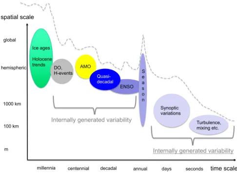
Fig. 2 Schematic diagram of the spatio-temporal scales considered. DO: Dansgaard-Oeschger, H: Heinrich events; AMO: Atlantic Multidecadal Oscillation; PDO: Pacidic Decadal Oscillation;
ENSO: El Ni˜no-Southern Oscillation. The annual and astronomical cycles are externally driven and have quasi-global impact. The dashed line shows a schematic power spectrum with more variability on long time scales.
In the entire climate system, different scales play an important role (Fig. 2). These are the characteristic orders of magnitude in space and time that a system possesses or is superimposed on the system in order to record or observe it. Climate has a spatial and temporal dimension, which fluctuate in a wide range of spatial and tem- poral scales. Spatial scales vary from local to regional to continental. Time scales vary from seasonal to geological. The spatio-temporal dimension of complex phe- nomena are defined by their typical spatial extension (e.g. the diameter of a high- pressure area), which is linked to a structure whose magnitudes can be specified as spatial scales. The time scale of an atmospheric process is the order of magnitude
of its lifetime. In addition, it is also possible to specify the spatial and temporal resolution with which a system is to be viewed. A distinction is made between the scale in space and time that an atmospheric process or an atmospheric system has and the scale of the observation. If the spatial and temporal scales of observation are to make it possible to capture the system in good resolution, they must be sig- nificantly smaller than those describing the overall system. The word ”scale” in this context means order of magnitude or scale. The spectrum of atmospheric space and time scales covers many orders of magnitude. A rough classification, which is com- mon in meteorology, is based on the horizontal space scale L. Basically, climate represents a space-time continuum, so that fixed scale limits do not occur in the real atmosphere. Rather, more or less narrow transition ranges between the scales are the rule. Larger and smaller systems influence each other so that the transitions between differently scaled weather phenomena are smooth and the approach is usually based on the question. In order to illustrate the scaling in the climate system, the procedure of non-dimensional parameters are introduced.
Models of planetary motion based on Newton’s models of gravity and motion, were astonishingly successful, and this had a profound impact on the way in which people viewed mathematical models and in the way that we still view them. The 18th century French scientist/mathematician Laplace, extended the basic Newto- nian model, given above, to model the motion of all the planets in the solar system, including their influences on each other. This model accounted for the motions of the planets as perfectly as they could be measured (including all the small devia- tions from elliptical orbits caused by the planets gravitational affects on each other).
This seemed to be such a triumph that the belief grew up that everything in the uni- verse could be described by such models, and that in principle the future could be predicted perfectly given such models and accurate measurements of the state of the universe now. Perhaps not surprisingly, Laplace was a vigorous promoter of this idea, which gained the name determinism.
These ideas lent their name to the concept of a deterministic model - that is a model which if solved from identical starting conditions always has the same solution. For much of the nineteenth century determinism reined, and resulted in a great deal of heart searching about free-will and the like. In the twentieth century three areas of science comprehensively overturned the idea that everything could be described by deterministic models. These were quantum mechanics and chaos theory. The later had its origin in meteorology and fluid dynamics.
In the 1960s, Edward Lorenz, a mathematician and meteorologist, showed that there are natural limits to the predictability of a nonlinear system, such as atmo- spheric circulation. He discovered and described the chaotic behaviour of large- scale motion patterns in the atmosphere and showed that despite the determinacy of the system, i.e. that although the partial differential equations could be calcu- lated at any time, the system itself loses its predictability after a relatively short time. Even the smallest changes in the initial conditions caused different final states after a few iteration steps (calculation steps). A predictability of the system is there- fore limited in time and the non-linearity is responsible for the finite predictability
of atmospheric flow patterns. This insight became known under the technical term
”butterfly effect”.
Climate physicists constantly trying to learn from our observations how to ex- amine causes and effects in such a way that the observations are captured. We write down our gained insights as mathematically formulated laws of nature. We formu- late equations of motion in the form of differential equations. Their solutions pro- vide information about what will happen to a given state at a given time at a later time. In this sense, the equations of motion as such provide a causal description par excellence - all equations of motion. Sometimes, however, there seem to be an- noying difficulties with causal chains or with predictability. For example, when the destructive path of a hurricane is poorly predicted, or in extreme weather events.
We are even more aware of the problems in long-term predictions, such as climate change. So is causality failing here? Of course we do not think so, otherwise we would not be looking for causes. It then also made no sense to derive political deci- sions from insights into climate evolution. And although word has got around that quantum mechanics is not a causal physics in the classical sense, we will hardly want to blame quantum mechanics for the cases of lack of predictability or unde- tectable cause-effect relationships. Here, the intersection of mathematical modeling and questions within Climate Change sciences are elaborated.
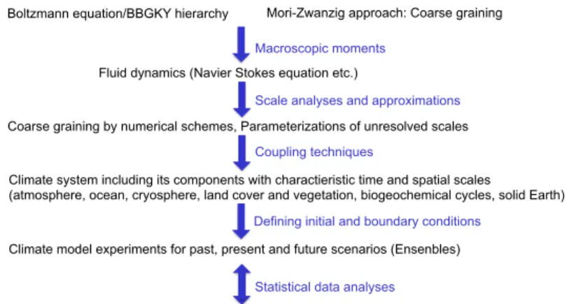
A systematic description of the mathematics and climate is given (Fig. 3). A general question within the micro-macro dynamic is that of integration between dif- ferent levels. Two distinctly different levels emerge with different rules governing each, but they then need to be reconciled in some way to create an overall function- ing system. Physical, chemical, biological, economic, social and cultural systems all exhibit this micro-macro dynamic and how the system comes to reconcile it forms a primary determinate in its identity and overall structure. This multi-dimensional nature to a system that results in the micro-macro dynamic is a product of synthesis and emergence. An approach is coarse graining and projection where the underly- ing dynamics is projected onto the macroscopic dynamics, the other is the statistical physics theory of non-equilibrium statistical mechanics. The Boltzmann equation, coarse graining, and the Brownian motion are the approaches to understand the dy- namics on different scales.
Climate: a fluid dynamical system
For present climate state we are able to directly measure all involved quantities.
From measurements we can draw conclusions about physical, chemical and bio- logical relationships between the variables. Our understanding about the involved processes is far from complete, but nevertheless we derive equations that describe and predict the observed phenomena.
Fluid dynamics (Navier Stokes equation etc.)
Boltzmann equation/BBGKY hierarchy Mori-Zwanzig approach: Coarse graining
Coarse graining by numerical schemes, Parameterizations of unresolved scales
Climate system including its components with charactieristic time and spatial scales
(atmosphere, ocean, cryosphere, land cover and vegetation, biogeochemical cycles, solid Earth) Macroscopic moments
Validation of climate scenarios on different time scales by using observations and paleoclimates Coupling techniques
Scale analyses and approximations
Climate model experiments for past, present and future scenarios (Ensenbles) Statistical data analyses
Defining initial and boundary conditions
Fig. 3 Systematic description of climate and mathematics. Changing the description of the dy- namics: from the micro to the macro scales. This is a common problem since we are not able to describe the systems on all temporal and spatial scales.
Mathematical equations
Our starting point is a mathematical model for the system of interest. In physics a model typically describes the state variables, plus fundamental laws and equations of state. These variables evolve in space and time. For the ocean, fundamental equa- tions are formulated:
• State variables: Velocity (in each of three directions), pressure, temperature, salinity, density
• Fundamental laws: Conservation of momentum, conservation of mass, conserva- tion of temperature and salinity
• Equations of state: Relationship of density to temperature, salinity and pressure, and perhaps also a model for the formation of sea-ice
The state variables are expressed as a continuum in space and time, and the funda- mental laws as partial differential equations. If the atmosphere is becoming too thin in the upper levels, a more molecular, statistical description is appropiate. Even at this stage, though, simplifications may be made. For example, it is common to treat seawater as incompressible. Furthermore, equations of state are often specified by empirical relationships or laboratory experiments.
∂ ρ
∂t +∇·(ρu) =0 (1)
or, using the substantive derivative:
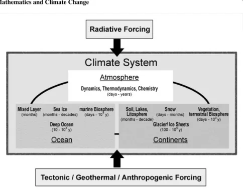
Fig. 4 Schematic view on the climate system. Global climate is a result of the complex interactions between the atmosphere, cryosphere (ice), hydrosphere (oceans), lithosphere (land), and biosphere (life), fueled by the non-uniform spatial distribution of incoming solar radiation (Peixoto and Oort 1992). We know from climate reconstructions using recorders such as ice cores, ocean and lake sediment cores, tree rings, corals, cave deposits, and ground water that the Earth’s climate has seen major changes over its history. An analysis of the temperature variations patched together from all these data reveals that climate change occurs in cycles with characteristic periods, for example 200 million, 100 thousand, or 4-7 years. For some of these cycles, particular mechanisms can be identified, for example forcing by changes in the Earth’s orbital parameters or internal oscillations of the coupled ocean-atmosphere system. However, major uncertainties remain in our understanding of the interplay of the components of the climate system.
Dρ
Dt +ρ(∇·u) =0. (2)
A simplification of the resulting flow equations is obtained when considering an in- compressible flow of a Newtonian fluid. The assumption of incompressibility rules out the possibility of sound or shock waves to occur; so this simplification is in- valid if these phenomena are important. The incompressible flow assumption typi- cally holds well even when dealing with a ”compressible” fluid -such as air at room temperature- at low Mach numbers (even when flowing up to about Mach 0.3).
The dynamics of flow are based on the Navier-Stokes equations. This is a state- ment of the conservation of momentum in a fluid and it is an application of Newton’s second law to a continuum; in fact this equation is applicable to any non-relativistic continuum and is known as the Cauchy momentum equation (e.g., Landau and Lif-
shitz (1959)). Taking this into account and assuming constant viscosity, the Navier- Stokes equations will read, in vector form:
Inertia (per volume)
z }| {
ρ ∂u
∂t
|{z}
Unsteady acceleration
+ u·∇u
| {z }
Advective acceleration
=
Divergence of stress
z }| {
−∇p
| {z }
Pressure gradient
+µ∇2u
| {z }
Viscosity
+ F
|{z}
Other body forces
. (3)
Note that only the advection terms are nonlinear for incompressible Newtonian flow.
This acceleration is an acceleration caused by a (possibly steady) change in velocity over position, for example the speeding up of fluid entering a converging nozzle.
Though individual fluid particles are being accelerated and thus are under unsteady motion, the flow field (a velocity distribution) will not necessarily be time depen- dent.
The vector fieldFrepresents ”other” (body force) forces. Typically this is only gravity, but may include other fields (such as electromagnetic). In a non-inertial coordinate system, other ”forces” such as that associated with rotating coordinates may be inserted. We note that the Coriolis force will be one of the main contribu- tions in the rotating Earth system. Often, these forces may be represented as the gradient of some scalar quantity. Gravity in the z direction, for example, is the gra- dient of−ρgz.Since pressure shows up only as a gradient, this implies that solving a problem without any such body force can be mended to include the body force by modifying pressure.
If temperature effects are also neglected, the only ”other” equation (apart from initial/boundary conditions) needed is the mass continuity equation. Under the in- compressible assumption, density is a constant and it follows that the equation will simplify to:
∇·u=0 . (4)
This is more specifically a statement of the conservation of volume (see divergence).
These equations are commonly used in 3 coordinates systems: Cartesian, cylindri- cal, and spherical. While the Cartesian equations seem to follow directly from the vector equation above, the vector form of the Navier-Stokes equation involves some tensor calculus which means that writing it in other coordinate systems is not as simple as doing so for scalar equations (such as the heat equation).
Taking the curl of the Navier-Stokes equation results in the elimination of pres- sure. This is especially easy to see if 2-dimensional Cartesian flow is assumed (w=0 and no dependence of anything on z), where the equations reduce to:
Dt ∇2ψ
=ν∇4ψ (5)
where∇4is the (2D) biharmonic operator andνis the kinematic viscosityν=µ
ρ. This single equation together with appropriate boundary conditions describes 2D fluid flow, taking only kinematic viscosity as a parameter. Note that the equation
for creeping flow results when the left side is assumed zero. In axisymmetric flow another stream function formulation, called the Stokes stream function, can be used to describe the velocity components of an incompressible flow with one scalar func- tion. The concept of taking the curl of the flow will become very important in climate dynamics (vorticity dynamics). The termζ =∇2ψ is called relative vorticity, and the term f=2Ωsinϕis due to the rotating Earth (Ω is the ratiation,ϕthe latitude).
The dynamics can be described by the barotropic vorticity equation as
Dt(ζ+f) =ν∇2ζ (6)
which is heavily used in climate research.
Non-dimensional parameters: The Reynolds number
In climate, we are interested in the critical paramters of the system. For the case of an incompressible flow in the Navier-Stokes equations, assuming the temperature effects are negligible and external forces are neglected, the equations consist of conservation of mass
∇·u=0 (7)
and momentum
∂tu+ (u·∇)u=−1 ρ0
∇p+ν∇2u (8) whereuis the velocity vector and p is the pressure,νdenotes the kinematic viscos- ity. The equations can be made dimensionless by a length-scale L, determined by the geometry of the flow, and by a characteristic velocity U. For inter-comparison of analytical solutions, numerical results, and of experimental measurements, it is useful to report the results in a dimensionless system. This is justified by the impor- tant concept of dynamic similarity (Buckingham (1914)). The main goal for using this system is to replace physical or numerical parameters with some dimensionless numbers, which completely determine the dynamical behavior of the system.
The procedure for converting to this system first implies, first of all, the selection of some representative values for the physical quantities involved in the original equations (in the physical system). For our current problem, we need to provide representative values for velocity(U),time(T),distances(L).From these, we can derive scaling parameters for the time-derivatives and spatial-gradients also. Using these values, the values in the dimensionless-system (written with subscript d) can be defined:
u=U·ud (9)
t =T·td (10)
x=L·xd (11)
withU=L/T. From these scalings, we can also derive
∂t = ∂
∂t = 1 T · ∂
∂td (12)
∂x= ∂
∂x= 1 L· ∂
∂xd (13)
Note furthermore the units of[ρ0] =kg/m3,[p] =kg/(ms2), and[p]/[ρ0] =m2/s2. Therefore the pressure gradient term has the scalingU2/L. Furthermore, divide the momentum equation byU2/L and the scalings vanish completely in front of the terms except for the∇2dud-term:
∇d·ud=0 (14) and conservation of momentum
∂
∂tdud+ (ud·∇d)ud=−∇dpd+ 1
Re∇2dud (15) The dimensionless parameterRe=U L/νis the Reynolds number and the only pa- rameter left.
For large Reynolds numbers, the flow is turbulent. In most practical flowsReis rather large(104−108),large enough for the flow to be turbulent. A large Reynolds number allows the flow to develop steep gradients locally. The typical length-scale corresponding to these steep gradients can become so small that viscosity is not neg- ligible. So the dissipation takes place at small scales. In this way different length- scales are present in a turbulent flow, which range from L to the Kolmogorov length scale. This length scale is the typical length of the smallest eddy present in a turbu- lent flow. In the climate system, this dissipation by turbulence is modeled via eddy terms. To evaluate the critical parameters and scales, we implicitly assume such procedure. A classical example is provided in the next section.
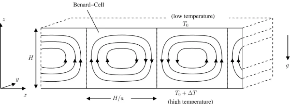
Convection in the Rayleigh-B´enard system
A system of three ordinary differential equations are introduced whose solutions afford the simplest example of deterministic flow that we are aware of. The system is a simplification of the one derived by Saltzman (1962), to study finite-amplitude convection.
Consider the Rayleigh-B´enard circulartion. Rayleigh (1916) studied the flow oc- curring in a layer of fluid of uniform depth H, when the temperature difference
Benard−Cell
(high temperature) (low temperature)
H/a H
T0+ ∆T x
y
z T0
g
Fig. 5 Geometry of the Rayleigh-B´enard system (see text for details).
between the upper- and lower-surfaces is maintained at a constant value∆T. T(x,y,z=H) =T0
T(x,y,z=0) = T0+∆T (16) The Boussinesq approximation is used, which results in a buoyancy force term which couples the thermal and fluid velocity fields. Therefore
ρ≈ρ0=const. (17)
except in the buoyancy term, where:
ρ=ρ0(1−α(T−T0))withα>0 . (18) ρ0 is the fluid density in the reference state. This assumption reflects a common feature of geophysical flows, where the density fluctuations caused by temperature variations are small, yet they are the ones driving the overall flow. We have the following relations. Furthermore, we assume that the density depends linearly on temperatureT.
This system possesses a steady-state solution in which there is no motion, and the temperature varies linearly with depth:
u=w=0 Teq=T0+
1− z H
∆T (19)
When this solution becomes unstable, convection should develop.
In the case where all motions are parallel to thex−z-plane, and no variations in the direction of the y-axis occur, the governing equations may be written (see Saltzman (1962)) as:
Dtu=−1 ρ0
∂xp+ν∇2u (20)
Dtw=−1 ρ0
∂zp+ν∇2w+g(1−α(T−T0)) (21)
DtT =κ∇2T (22)
∂xu+∂zw=0 (23)
wherewanduare the vertical and horizontal components of the velocity. Further- more,ν=η/ρ0,κ=λ/(ρ0Cv)the momentum diffusivity (kinematic viscosity) and thermal diffussivity, respectively.
Now, the pressure is eliminated to derive the vorticity equation Dt ∇2ψ
= ν∇4ψ. Here, it is useful to define the stream functionΨ for the two-dimensional motion, i.e.
∂Ψ
∂x =w (24)
∂Ψ
∂z =−u . (25)
∂
∂x(21)− ∂
∂z(20) = ∂
∂xDtw− ∂
∂zDtu=Dt∂w
∂x−Dt∂u
∂z (26)
= =Dt
∂2Ψ
∂x2 −Dt
∂2Ψ
∂z2 =Dt∇2Ψ . (27) Furthermore, one can introduce the functionΘas the departure of temperature from that occurring in the state of no convection (19):
T=Teq+Θ (28)
In the temperature term in ∂
∂x(21)on the right hand side:
∂
∂xg(1−α(Teq+Θ−T0)) =−gα ∂
∂xΘ The left hand side of (22) reads
DtT =DtTeq+DtΘ =w·−∆T
H +DtΘ=−∆T H
∂Ψ
∂x +DtΘ
Then, the dynamics can be formulated as Dt ∇2Ψ
=ν∇4Ψ−gα∂Θ
∂x (29)
DtΘ =∆T H
∂Ψ
∂x +κ∇2Θ . (30)
Non-dimensionalization of the problem yields equations including the dimen- sionless Prandtl numberσ and the Rayleigh numberRawhich are the control pa- rameters of the problem. One can take the layer thickness H as the length of unit, the timeT =H2/κof vertical diffusion of heat as the unit of time, and the temperature difference∆T as the unit of temperature.
Reduction of dimensions and the Lorenz system
Saltzman (1962) derived a set of ordinary differential equations by expandingΨand Θ in double Fourier series inxandz, with functions oftalone for coefficients, and substituting these series into (29) and (30) A complete Galerkin approximation
Ψ(x,z,t) =
∞ k=1
∑
∞ l=1
∑
Ψk,l(t)sin kπa
H x
×sin lπ
Hz
(31) Θ(x,z,t) =
∞ k=1
∑
∞ l=1
∑
Θk,l(t)cos kπa
H x
×sin lπ
Hz
(32) yields an infinite set of ordinary differential equations for the time coefficients. He arranged the right-hand sides of the resulting equations in double Fourier-series form, by replacing products of trigonometric functions of x (or z) by sums of trigonometric functions, and then equated coefficients of similar functions ofxandz.
He then reduced the resulting infinite system to a finite system by omitting reference to all but a specified finite set of functions oft. He then obtained time-dependent so- lutions by numerical integration. In certain cases all, except three of the dependent variables, eventually tended to zero, and these three variables underwent irregular, apparently non-periodic fluctuations. These same solutions would have been ob- tained if the series had been at the start truncated to include a total of three terms.
Accordingly, in this study we shall let a
1+a2κ Ψ=X
√
2 sinπa Hx
sinπ Hz
(33) πRa
Rc 1
∆T Θ=Y√
2 cosπa Hx
sinπ Hz
−Zsin 2π
Hz
(34) whereX(t),Y(t), andZ(t)are functions of time alone.
It is found that fields of motion of this form would develop if the Rayleigh num- ber
Ra=gαH3∆T
ν κ , (35)
exceeds a critical value
Rc=π4a−2(1+a2)3 . (36) The minimum value ofRc, namely 27π4/4=657.51, occurs whena2=1/2. In fluid mechanics, the Rayleigh number for a fluid is a dimensionless number associated
with the relation of buoyancy and viscosity in a flow. When the Rayleigh number is below the critical value for that fluid, heat transfer is primarily in the form of conduction; when it exceeds the critical value, heat transfer is primarily in the form of convection.
When the above truncation (33,34) is substituted into the dynamics, we obtain the equations (Lorenz model):
X˙ =−σX+σY (37)
Y˙ =rX−Y−X Z (38)
Z˙=−bZ+XY (39)
Here a dot denotes a derivative with respect to the dimensionless timetd=π2H−2(1+ a2)κt, whileσ=ν κ−1is the Prandtl number,r=Ra/Rc, andb=4(1+a2)−1.
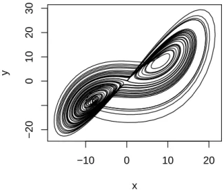
Equations (37, 38, 39) are calledLorenz modelin the literature (Lorenz 1960, 1963, 1984; Maas 1994; Olbers 2001). The system may give realistic results when the Rayleigh number is slightly supercritical, but their solutions cannot be expected to resemble those of the complete dynamics when strong convection occurs, in view of the extreme truncation. Figure 6 shows the numerical solution in the phase-space with the parametersr=28, σ=10, andb=8/3. The chaotic nature of this system inspired climate scientist and scientists in general. This phenomenon had probably the greatest impact of climate science to mathematics.
−10 0 10 20
−200102030
LORENZ ATTRACTOR
x
y
Fig. 6 Numerical solution of the Lorenz model, in theX−Y phase-space with the parameters r=28,σ=10, andb=8/3.
Scaling in the climate system
As we will see now, the Coriolis effect is one of the dominating forces for the large- scale dynamics of the oceans and the atmosphere. It is convenient to work in the rotating frame of reference of the Earth. The equation can be scaled by a length- scale L, determined by the geometry of the flow, and by a characteristic velocity U. One can estimate the relative contributions in units of m/s2 in the horizontal momentum equations:
∂v
∂t
|{z}
U/T∼10−8
+ v·∇v
| {z }
U2/L∼10−8
= −1 ρ∇p
| {z }
δP/(ρL)∼10−5
+2ΩΩΩ×v
| {z }
f0U∼10−5
+ f ric
|{z}
νU/H2∼10−13
(40)
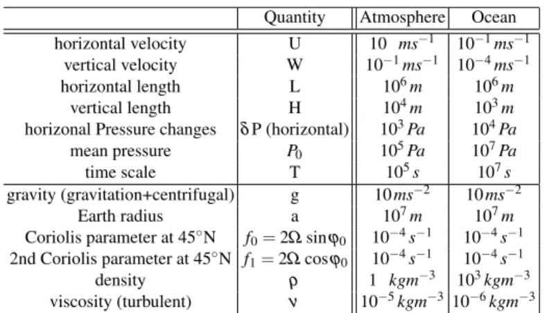
where fric denotes the contributions of friction due to eddy stress divergence (usu- ally∼ν∇2v). Typical values are given in Table 1. The values have been taken for theocean.
It is furthermore useful to think about the orders of magnitude: Because of the continuity equationU/L∼W/Hand since the horizontal scales are orders of mag- nitude larger than the vertical ones, the vertical velocity is very small relative to the horizontal. For small scale motion (like small-scale ocean convection or cumulus clouds) the horizontal length scale is of the same order as the vertical one and there- fore the vertical motion is in the same order of magnitude as the horizontal motion.
The timescales are related toT∼L/U∼H/W.
It is essential to think about the relative importance of the different terms in the momentum balance (40). The Rossby Number Ro is the ratio of inertial (the left hand side) to Coriolis (second term on the right hand side) terms
Ro=(U2/L) (f U) = U
f L . (41)
It is used in the oceans and atmosphere, where it characterizes the importance of Coriolis accelerations arising from planetary rotation. It is also known as the Kibel number. Ro is small when the flow is in a so-called geostrophic balance.
Projection methods: coarse graining and stable manifold theory
The structure of fluid dynamical models and thus climate models is valid for sys- tems with many degrees of freedom, many collisions, and for substances which can be described as a continuum. The transition from the highly complex dynamical equations to a reduced system is an important step since it gives more credibility to the approach and its results. The transition is also necessary since the active en- tangled processes are running on spatial scales from millimetres to thousands of kilometres, and temporal scales from seconds to millennia (Figs. 2, 3). Therefore,
Quantity Atmosphere Ocean horizontal velocity U 10 ms−1 10−1ms−1
vertical velocity W 10−1ms−1 10−4ms−1
horizontal length L 106m 106m
vertical length H 104m 103m
horizonal Pressure changes δP (horizontal) 103Pa 104Pa
mean pressure P0 105Pa 107Pa
time scale T 105s 107s
gravity (gravitation+centrifugal) g 10ms−2 10ms−2
Earth radius a 107m 107m
Coriolis parameter at 45◦N f0=2Ωsinϕ0 10−4s−1 10−4s−1 2nd Coriolis parameter at 45◦N f1=2Ωcosϕ0 10−4s−1 10−4s−1
density ρ 1 kgm−3 103kgm−3
viscosity (turbulent) ν 10−5kgm−310−6kgm−3
Table 1 Table shows the typical scales in the atmosphere and ocean system. Using these orders of magnitude, one can derive estimates of the different terms in (40).
the unresolved processes on subgrid scales have to be described. This is the typical problem in statistical physics, known as the so-called Mori-Zwanzig approach (Mori 1965; Zwanzig 1960, 1980). The basic idea is the evolution of a system through a projection on a subset (macroscopic relevant part), where a randomness reflects the effects of the unresolved degrees of freedom. A particular example is the Brownian motion (Einstein 1905; Langevin 1908). Another solution for the transition form may degrees of freedom to the macroscopic laws goes back to Boltzmann (1896).
The Boltzmann equation, also often known as the Boltzmann transport equation (Boltzmann 1896; Bhatnagar et al 1954; Cercignani 1990) describes the statistical distribution of one particle in a fluid. It is one of the most important equations of non-equilibrium statistical mechanics, the area of statistical mechanics that deals with systems far from thermodynamic equilibrium. It is applied, for instance, when there is an applied temperature gradient or electric field. Both, the Mori-Zwanzig and Boltzmann approaches play also a fundamental role in physics. The microscopic equations show no preferred time direction, whereas the macroscopic phenomena in the thermodynamics have a time direction through the entropy. The underlying pro- cedure is that part of the microscopic information is lost through coarse graining in space and time.
In order to get a first idea of coarse graining, one one may think of the transi- tion from Rayleigh-B´enard convection to the Lorenz system (sectionConvection in the Rayleigh-B´enard system). In our formula, the Galerkin approximation (32,32) provided a suitable projector to simply truncate the series at some specified wave number cut-off into a low-order system (such as in equations (33, 34). The mathe- matical theory behind this truncation is called the center manifold theory (Oseledets 1968; Haken 1983). We could arrive at the slow manifold of the climate system, to which all the faster response variables (e.g., the atmosphere) are attracted. In math- ematics, the slow manifold of an equilibrium point of a dynamical system occurs as the most common example of a center manifold. One of the main methods of sim-
plifying dynamical systems, is to reduce the dimension of the system to that of the slow manifold—center manifold theory rigorously justifies the modelling (Lorenz 1986; Arnold 1998; Roberts 2008; Arnold and Imkeller 1998).
The Mori-Zwanzig formalism (Mori 1965; Zwanzig 1960) and the slow manifold theory provide a conceptual framework for the study of dimension reduction and the parameterization of less relevant variables by a stochastic process. It includes a gen- eralized Langevin (1908) theory. Langevin (1908) studied Brownian motion from a different perspective to Einstein’s seminal 1905 paper (Einstein 1905), describ- ing the motion of a single Brownian particle as a dynamic process via a stochastic differential equation, as an Ornstein-Uhlenbeck process (Uhlenbeck and Ornstein 1930).
The Gaussian filtering of hydrodynamic equations that leads to the Smagorinsky equations (Smagorinsky 1963) is, in its essence, a version of coarse-graining. The projection method includes the procedure to describe turbulent energy dissipation in turbulent flows, where the larger eddies extract energy from the mean flow and ultimately transfer some of it to the smaller eddies which, in turn, pass the energy to even smaller eddies, and so on up to the smallest scales, where the eddies convert the kinetic energy into internal energy of the fluid. At this scales (also known as Kolmogorov scale), the viscous friction dominates the flow (Frisch 1996).
Brownian motion, weather and climate
The daily observed maximum and minimum temperatures is often compared to the
”normal” temperatures based upon the 30-year average. Climate averages provide a context for something like ”this winter will be wetter (or drier, or colder, or warmer, etc.) than normal. It has been said ”Climate is what you expect. Weather is what you get.” What is the difference between weather and climate? This can be also answered by an example/a metaphor in the football league. Predicting the outcome of the next game is difficult (weather), but predicting who will end up as German champion is unfortunately relatively easy (climate).
For climate, this transition between the climate and weather scales has been for- mulated conceptually (Hasselmann 1976; Leith 1975), and later re-formulated in a mathematical context (Arnold 2001; Chorin et al 1999; Gottwald 2010). The ef- fect of the weather on climate is seen by red-noise spectra in the climate system, showing one of the most fundamental aspects of climate, and serving also as a null hypothesis for climate variability studies.
In a stochastic framework of climate theory one may use an appropriate stochas- tic differential equation (Langevin equation)
d
dtx(t) = f(x) +g(x)ξ, (42)
whereξ= d
dtW(t)is a stationary stochastic process and the functions f,g:Rn→Rn describe the climate dynamics. The properties of the random force are described through its distribution and its correlation properties at different times. The process ξ is assumed to have a Gaussian distribution of zero average,
<ξ(t)>=0 (43)
and to beδ-correlated in time,
<ξ(t)ξ(t+τ)>=δ(τ) (44)
whereδ is the delta function defined by Z
R
f(x)δ(x−x0)dx=f(x0) . (45) The brackets indicate an average over realizations of the random force. Formally:
ξ(t)is a random variable, i.e. ξ(t)(α) with different realizations due to random variableα. The expectation<ξ(t)>is thus the mean over allα:<ξ(t)(α)>α. Using the ergodic hypothesis, the ensemble averagehican be expressed as the time average limT→∞1
T RT/2
−T/2dtof the function. Almost all points in any subset of the phase space eventually revisit the set. For a Gaussian process only the average and second moment need to be specified since all higher moments can be expressed in terms of the first two. Note that the dependence of the correlation function on the time differenceτ assumes thatξ is a stationary process.ξ is called a white-noise process.
Additionally, there might be an external forcingF(x,t)which is generally time- , variable-, and space-dependent. In his theoretical approach, Hasselmann (1976) formulated a linear stochastic climate model
d
dtx(t) =Ax+σ ξ+F(t) , (46) with system matrix A∈Rn×n, constant noise term σ, and stochastic process ξ. Many features of the climate system can be well described by (46), which is analo- gous to the Ornstein-Uhlenbeck process in statistical physics (Uhlenbeck and Orn- stein 1930). Notice thatσ ξrepresents a stationary random process. The relationship derived above is identical to that describing the diffusion of a fluid particle in a tur- bulent fluid. In a time-scale separated system, during one slow-time unit the fast uninteresting variablesyperform many ’uncorrelated’ events (provided that the fast dynamics are sufficiently chaotic). The contribution of the uncorrelated events to the dynamics of the slow interesting variables x is as a sum of independent random variables. By the weak central limit theorem this can be expressed by a normally distributed variable. Note, in the absence of any feedback effectsAx, the climate variations would continue to grow indefinitely as the Wiener process. A perturba- tion in a system with a negative feedback mechanism will be reduced whereas in a system with positive feedback mechanisms, the perturbation will grow. In the one
dimensional case,Acan be rewritten as−λ. The real part ofλ determines then the stability of the system and is called feedback factor.
Climate variability and sensitivity
Imagine now that the temperature of the ocean mixed layer of depth h is governed by a one-dimensional system
dT
dt =−λT+Qnet+f(t), (47) where the air-sea fluxes due to weather systems are represented by a white-noise process with zero average<Qnet>=0 andδ-correlated in time<Qnet(t)Qnet(t+
τ)>=δ(τ). The function f(t)is a time dependent deterministic forcing. Assume
furthermore that f(t) =c·u(t) withu(t) as unit step or the so-called Heaviside step function. Because<Qnet >=0,<T(t)>can be solved using the Laplace transform:
<T(t)>=L−1{F(s)}(t) =L−1<T(0)>
s+λ +c s· 1
s+λ
(48)
=T(0)·exp(−λt) + c
λ(1−exp(−λt)) (49) because we have<T(0)>=T(0). As equilibrium response, we have
∆T =lim
t→∞<T(t)>= c
λ. (50)
The fluctuation can be characterized by the spectrum S(ω) =<TˆTˆ∗>= 1
λ2+ω2. (51)
and therefore, the spectrum and the equilibrium response are closely coupled ( fluctuation-dissipation theorem). In mathematics, this is called Wiener-Chintschin- Theorem (Wiener 1930; Chintchin 1934). For some energy considerations, it is use- ful to re-write equation (47) as
CdT
dt =−λCT+fC, (52)
withC=cpρdzas the heat capacity of the ocean. For a depth of 200 m of water distributed over the globe,C=4.2·103W s kg−1K−1×1000kg m−3×200m=8.4· 108W s m−2K−1.The temperature evolution is
T(t) =T(0)·exp(−λc/C t) + fC λC
(1−exp(−λC/C t)) (53)
The left hand side of (52) represents the heat uptake by the ocean, which plays a central role in the transient response of the system to a perturbation (53).
Typical changes in fC are 4W m−2for doubling ofCO2,λC=1−2W m−2K−1. The typical time scale for a mixed layer ocean isC/λC=13−26 years . Please note that the climate system is simplified by a slab ocean with homogeneous temperature and heat capacity. This is an approximation as the heat capacity should vary in time as the perturbation penetrates to deeper oceanic levels. The equilibrium temperature change∆T is
∆T =∆fC λC = c
λ (54)
with values of∆T =2−4 K. The termCS= 1
λC is called climate sensitivity to a radiative forcing∆fC:
∆T =CS· ∆fC . (55)
In the literature, the concept of climate sensitivity is quite often used as the equilib- rium temperature increase for a forcing∆fCrelated to doubling ofCO2. It is obvious that the CS depends on the included sources of feedback of the system which are re- lated to climate components and their respective time scales (e.g., Lohmann (2018)).
Due to the non-normality in (46), the effective damping may not be directly related to the eigenvalues of the system.
Non-normal growth of the climate system
In the one-dimensional case for x(t) =exp(at)we have the the inverse Laplace transform
exp(at) =L−1{F(s)}(t) = 1 2πi lim
T→∞
Z γ+iT γ−iT est 1
s−ads, (56) and and the entire range of t is controlled t by the resolvent|s−a1 |.Using the Fourier transformation, (46) with forcing F(t) is tranformed to
(iωI−A)xˆ=Fˆ (57)
ˆ
x= (iωI−A)−1Fˆ (58) where I is the identity. The so-called resolvent operator of matrix A is R(ω) = (iωI−A)−1 The behavior of the norms ||exp(At)|| over the entire range of t is controlled t by the resolvent norm||R(ω)||. If A is a normal operator
A A+ = A+A , (59)
where+denotes the adjoint-complex operator, then
||R(ω)||=1/dist(iω,σ(A)) (60) is completely determined by the spectrumσ(A)alone. The operator dist denotes the shortest distance ofω to the eigenvalues, the spectrumσ(A). This explains the success of eigenvalue analysis. In contrast to this, for non-normal operators the be- havior of ||R(ω)|| may deviate from that dramatically and hence in this context pseudospectral analysis is just the right tool For example, there are problems in fluid mechanics whereσ(A)is contained in the left half-plane, which suggests lam- inar behavior, but it protrudes strongly into the right half-plane, which implies that
||eAt||has a big hump before decaying exponentially fast to zero Reddy et al (1993);
Trefethen et al (1993). More about the dynamics can be learned by examining the pseudospectrum ofAin the complex plane. Inspection of many geophysical systems shows that most of the systems fail the normality condition. Theε−pseudospectrum of operatorAis defined by two equivalent formulations:
Λε(A) ={z∈C:||(zI−A)−1|| ≥ε−1}
={z∈C:[smallest singular value of(zI−A)]≤ε} . (61) This set of valueszin the complex plane are defined by contourlines of the resolvent (zI−A)−1.The resolvent determines the system’s response to a forcing as supplied by external forcingF(x,t),stochastic forcingg(x)ξ,or initial/boundary conditions.
The pseudospectrum reflects the robustness of the spectrum and provides informa- tion about instability and resonance. One theorem is derived from Laplace trans- formation stating that transient growth is related to how far theε−pseudospectrum extends into the right half plane:
||exp(At)|| ≥ 1 ε sup
z∈Λε(A)
Real(z) . (62)
In terms of climate theory, the pseudospectrum indicates resonant amplification.
Maximal amplification is at the poles of(zI−A)−1,characterized by the eigenfre- quencies. In a mathematical normal matrix A, the system’s response is characterized solely by the proximity to the eigenfrequencies. In the non-normal case, the pseu- dospectrum shows large resonant amplification for frequencies which are not eigen- frequencies. This transient growth mechanism is important for both initial value and forced problems.
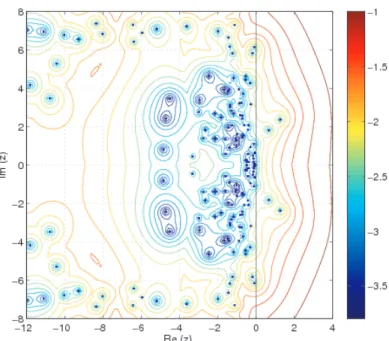
An atmospheric general circulation model PUMA Fraedrich et al (2005) is ap- plied to the problem. The model is based on the multi-level spectral model described by Hoskins and Simmons Hoskins and Simmons (1975). For our experiments we chose five vertical levels and a T21 horizontal resolution. PUMA belongs to the class of models of intermediate complexity Claussen et al (2002); it has been used to un- derstand principle feedbacks Lunkeit et al (1998), and dynamics on long time scales Romanova et al (2006). For simplicity, the equations are scaled here such that they are dimensionless. The model is linearized about a zonally symmetric mean state
providing for a realistic storm track at mid-latitudes Frisius et al (1998). In a simpli- fied version of the model and calculating the linear modelAwithn=214, one can derive the pseudospectrum. Fig. 7 indicates resonances besides the poles (the eigen- values) indicated by crosses. TheIm(z)−axis shows the frequencies, theRe(z)−axis the damping/amplification of the modes. Important modes for the climate system are those with−0.5<Im(z)<0.5 representing planetary Rossby waves. The basic feature is that transient growth of initially small perturbations can occur even if all the eigenmodes decay exponentially. Mathematically, an arbitrary matrixAcan be decomposed as a sum
A=D+N (63)
whereAis diagonalizable, andN is nilpotent (there exists an integer q∈N with Nq=0), andDcommutes withN(i.e.DN=NA).This fact follows from the Jordan- Chevalley decomposition theorem. This means that we can compute the exponential of (A t) by reducing to the cases:
exp(At) =exp( (D+N)t) =exp(Dt) exp(Nt) (64) where the exponential ofNtcan be computed directly from the series expansion, as the series terminates after a finite number of terms. Basically, the numberq∈Nis related to the transient growth of the system (q=1 means no transient growth).
The resonant structures are due to the mode interaction: It is not possible to change one variable without the others, because they are not orthogonal. Interest- ingly, one can also compute theA+ model, showing the optimal perturbation of a mode through its biorthogonal vector which is the associated eigenvector of the ad- jointA+. The analysis indicates that non-normality of the system is a fundamental feature of the atmospheric dynamics. This has consequences for the error growth dynamics, and instability of the system, e.g. Palmer (1996); Lohmann and Schnei- der (1999). Similar features are obtained in shear flow systems Reddy et al (1993);
Trefethen et al (1993) and other hydrodynamic applications. This transient growth mechanism is important for both initial value and forced problems of the climate system Farrell and Ioannou (1996).
Predictability
In climate we may ask about our initial state? Climatologists always feel uncertain when we want to give the initial values. There is always a more or less big inaccuracy due to weather and uncertainties in many quantities which cannot be observed at any time step (e.g. the deep ocean). The Lyapunov exponentsλ play an important role in knowing the predictability of a system. This is because the larger they are, the smaller the number of steps for which predictions can be made with a certain, desired accuracy. Consider a trajectoryx(t)and a nearby trajectoryx(t)+δ(t)where δ(t)is a vector with infinitesimal initial length. As the system evolves, track how
Fig. 7 Contours of log10(1/ε).The figure displays resonant structures of the linearized atmo- spheric circulation model. The modes extend to the right half plane and are connected through resonant structures, indicating for transient growth mechanism inherent in atmospheric dynamics.
δ(t)changes. The maximal Lyapunov exponent of the system is the numberλsuch that|δ(t)| ≈ |δ(0)| ·exp(λt).A classical example is again the Lorenz system (37, 38, 39) where for large parts of the phase space, we have limited predictability because initial errors can grow.
Every dynamical system has a spectrum of Lyapunov exponents, one for each dimension of its phase space. Like the largest eigenvalue of a matrix, the largest Lyapunov exponent is responsible for the dominant behavior of a system. In case of weather and climate, this Lyapunov exponent is therefore also time-scale dependent.
Causality in climate has only a limited range in time and can only be verified in the context of finite errors. Please note that even in classical mechanics, strict causal relationships cannot be verified experimentally! It is true that the classical laws of motion are generally deterministic. But the connection with the real physical world is always possible only with limited accuracy due to the unavoidable measurement errors. Therefore, the actual state can only be given with a certain probability distri- bution within state ranges. In the usual discussion this important part of physics is often faded out, one likes to limit oneself to the equations of motion alone.
Natural events also have their own time scales, namely the so-called Lyapunov timestLyap (these result from the expansion rates attLyap=λ−1). This Lyapunov time of a weather situation, it is about seconds to days, for climate years to decades.
We now have to compare the two relevant time scalestMandtLyap. Three cases are possible:
• The Lyapunov time of the climate system under investigation is much larger than the humanly relevant time scale (tLyap>>tM): Then we can imagine the initial state inaccuracy to be smaller and smaller in our minds, because this would only increase the prediction time. Even if it would become infinite in our thoughts because we let the measurement inaccuracy become zero, we would not even notice it. Therefore, in these cases we consider the event (within the accepted accuracy) to be predictable, causal.
• The human relevant time scale is much larger than the Lyapunov time of the in- vestigated system (tM>>tLyap): In this case prediction is no longer possible, the actual course is completely different from the expected one. We observe statisti- cal, random behaviour, since we do not know the actual initial state.
• The relevant time scale is about as large as the Lyapunov time of the system un- der study (tM ≈tLyap): Then no exact but approximate predictions are possible;
it is also not entirely random, statistically. The predictions can even be improved by measurement progress or by less demanding requirements for prediction ac- curacy. A good example is the weather forecasts, which are only possible to a limited extent; in the short and medium term they are now quite reliable.
In essence, therefore, causality depends on the time of interest in comparison to the forecast time, whether we can regard a phenomenon ”practically” as causal, as predictable in (sometimes excellent approximation), or whether the event appears to us to be completely random, or finally as lying in the transition area and is therefore experienced as improvable by increasing the accuracy, i.e. as neither causal nor sta- tistical. Climate is not only a differential equation; it must also be coupled to the real world by specifying the initial values with measurement errors and by translating the final values into measurable predictions. Thus it loses its purely mathematical, causal character determined by the solution of differential equations.
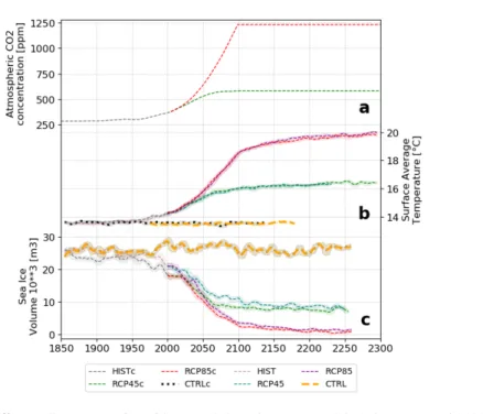
Besides the initial conditions, uncertainties can appear through the external forc- ing. Prominent external forcing are the change in greenhouse gases into the atmo- sphere (e.g., Fig. 8) which strongly affect the long-term evolution of the Earth sys- tem. Another external forcing is due to changes in insolation by orbital parameters.
There parameters vary on multi-millennial time scales (thousand years=ky) and can be calculated by orbital theory. Milankovitch Milankovitch (1941) suggested the ice sheet growth and decay is triggered by this external forcing. There are several open questions for paleoclimate dynamics. Despite the pronounced change in Earth system response evidenced in paleoclimatic records, the frequency and amplitude characteristics of the orbital parameters, i.e. eccentricity (∼100 ky), obliquity (∼41 ky) and precession (∼21 and∼19 ky), do not vary Berger and Loutre (1991), the climate frequency does. The uncertainty on long time scale is usually dominated by the external forcing, the short time scale by the initial value problem, the intermedi- ate times at 10-50 years for the coming decades are dominated by internal variabil- ity and uncertainty in model physics (Hawkins and Sutton 2009). The uncertainty of global and especially regional temperature estimates on decadal to multi-decadal time scales are manifested by large-scale coherent pattern like AMO, PDO, and the the quasi-decadal mode (cf. Fig. 2). For a while people tended to think that determin- istic models would still always provide the best models in these cases. One thought
Fig. 8 Different climate scenarios with a coupled Earth system model (Ackermann et al 2020).
Time series of 11-year mean (a) CO2 forcing as concentration of CO2equivalent in the atmo- sphere, (b) global near-surface average temperature, (c) sea ice volume in the Northern Hemi- sphere; shaded areas indicate 1 standard deviation;
of the climate system is that deterministic models would be completely adequate for describing the Earth’s atmosphere, which is basically just a layer of gas subject to external heating. As seen here, the phenomenon of stochasticity means that this is not so. As in the Lorenz system, chaos is introduced into the climate system. So, in many cases, for quite fundamental reasons, deterministic mathematical models do not provide adequate models. Statistical models are mathematical models, each replicate realization of which will be different from other realizations with the same model, even under identical conditions. Statistical models are the major means of making sense of the climate dynamics.
Boltzmann Dynamics
One of the most significant theoretical breakthroughs in statistical physics was due to Ludwig Boltzmann (Boltzmann (1896), Boltzmann (1995) for a recent reprint of his famous lectures on kinetic theory), who pioneered non-equilibrium statistical mechanics. Boltzmann postulated that a gas was composed of a set of interacting particles, whose dynamics could be (at least in principle) modelled by classical dy-
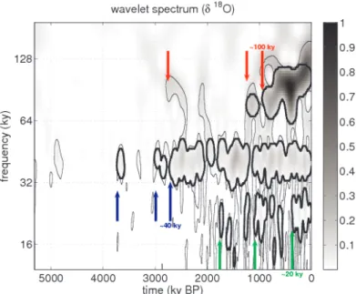
Fig. 9 The wavelet sample spectrum of long-term climate change. The climate record is based on Lisiecki and Raymo Lisiecki and Raymo (2005). The wavelet is calculated using Morlet wavelet withω0=6.Thin and thick lines surround pointwise and areawise significant patches, respectively.
namics. Due to the very large number of particles in such a system, a statistical approach was adopted, based on simplified physics composed of particle streaming in space and billiard-like inter-particle collisions (which are assumed elastic).
As already mentioned above, a fluid can be described by several physical theo- ries, of different granularities. The fact that we can, in principle, recover the phe- nomena predicted by the coarse-grained theories from solutions of the fine-grained theories also suggests a non-conventional way of constructing numerical algorithms for simulating fluid flows: instead of directly modeling the coarse-grained equations (i.e. Navier-Stokes equations for human-scale flows), we can construct a simplified model of the fine-grained equations, which will exhibit the same behavior at the larger scales.
In the following, an example derived for the Lattice Boltzmann Model (LBM) is shown which is related the thermohaline circulation. Water, that is dense enough to sink from the surface to the bottom, is formed when cold air blows across the ocean at high latitudes in winter in the northern North Atlantic (e.g. in the Labrador Sea and between Norway and Greenland) and near Antarctica. The wind cools and evaporates water. If the wind is cold enough, sea ice forms, further increasing the salinity of the water because sea ice is fresher than sea water and salty water remains in the water when ice is formed. Bottom water is produced only in these regions, and the deep ocean is affected by these deep water formation processes. In other regions, cold, dense water is formed, but it is not quite salty enough to sink to the bottom. At
mid and low latitudes, the density, even in winter, is sufficiently low that the water cannot sink more than a few hundred meters into the ocean. The only exception are some seas, such as the Mediterranean Sea, where evaporation is so great that the salinity of the water is sufficiently great for the water to sink to intermediate depths in the seas. If these seas are can exchange water with the open ocean, the waters formed in winter in the seas spreads out to intermediate depths in the ocean.
A numerical solution of this equation is shown in Fig. 10.
(a) Two hemisphere temperature (b) Ridge and a two hemisphere temperature
(c) Linear temperature gradient (d) Flow including a ridge
Fig. 10 Four examples of the ocean flow for different boundary conditions, and fixed Prandtl number=1 and Rayleigh number=45000. The contours show lines of constant vorticity; the colors in the background display the temperatures (purple - warm, blue - cold). For the right scenarios, an obstacle representing an oceanic sill is implemented.
Conclusions
Climate change occurred during the history of the Earth, the tectonic movements over billions of years, and climate has varied between extremes before any an- thropogenic action could have arisen. However, anthropogenic action in terms of heavy usage of fossil fuel has the potential to affect the Earth to a point where its habitability is significantly affected. In terms of the time scale, it is noted that we might disturb planetary-scale processes in the course of a few decades. The complication is due to the fact that the climate system has inherent fluctuations (internal climate variability), uncertainties in model formulations, and scenario un-
![Fig. 1 Northern Hemisphere near-surface temperature anomaly [K] based on HadCRUT4 (Morice et al 2012).](https://thumb-eu.123doks.com/thumbv2/1library_info/5202521.1668248/2.918.248.652.300.461/northern-hemisphere-surface-temperature-anomaly-based-hadcrut-morice.webp)