Characterization of cis-regulatory elements via open chromatin profiling
D i s s e r t a t i o n
zur Erlangung des akademischen Grades Ph.D.
bzw. Doctor of Philosophy im Fach Biologie eingereicht an der
Lebenswissenschaftlichen Fakultät der Humboldt-Universität zu Berlin von
MSc Aslihan Karabacak Calviello Präsidentin der Humboldt-Universität zu Berlin
Prof. Dr.-Ing. Dr. Sabine Kunst
Dekan der Lebenswissenschaftlichen Fakultät der Humboldt-Universität zu Berlin Prof. Dr. Bernhard Grimm
Gutachter/innen:
1 – Prof. Dr. Uwe Ohler 2 – Prof. Dr. Stein Aerts 3 – Dr. David Garfield
Tag der mündlichten Prüfung 24.01.2019
i
Contents
Abstract ... v
Zusammenfassung ... vi
1. Introduction ... 1
1.1 Thesis outline ... 2
2. Background ... 4
2.1. Transcriptional regulation of gene expression ... 4
2.1.1. Chromatin ... 4
2.1.2. Cis-regulatory elements ... 5
2.1.3. Transcription factors ... 7
2.2. Drosophila melanogaster as a model organism of embryogenesis ... 7
2.2.1. Specification of the mesoderm ... 8
2.2.2. Specification of the neurogenic ectoderm ... 8
2.3. Genome-wide sequencing techniques to identify and characterize cis-regulatory elements ... 9
2.3.1. Next-generation sequencing ... 9
2.3.2. Techniques to profile transcription factor binding sites and histone modifications ... 11
2.3.2.1. ChIP-seq ... 12
2.3.2.2. BiTS-ChIP ... 13
2.3.3. Techniques to profile open chromatin... 14
2.3.3.1. DNase-seq ... 14
2.3.3.2. ATAC-seq ... 16
2.4. Computational analysis of genome-wide sequencing datasets ... 18
2.4.1. Read processing, alignment and filtering ... 18
2.4.2. Finding regions of enrichment via peak calling ... 19
2.4.3. Finding transcription factor binding sites ... 21
2.4.3.1. Position weight matrices ... 21
2.4.3.2. Transcription factor footprinting ... 23
3. Materials and Methods ... 25
3.1 DNase-seq and ATAC-seq experimental procedures and data preprocessing ... 25
3.2 Peak calling ... 29
3.3 Sequence bias of DNase I and Tn5 transposase ... 31
3.4 Scanning the genome for candidate binding sites ... 32
3.5 Identification of transcription factor footprints ... 34
3.6 Differential signal analyses ... 35
ii
3.7 Motif enrichment analyses ... 36
3.8 Integrative model of TF binding ... 37
4. Results ... 38
4.1. Part 1: Reproducible inference of regulatory regions and transcription factor footprints using open chromatin profiling data ... 38
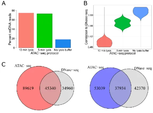
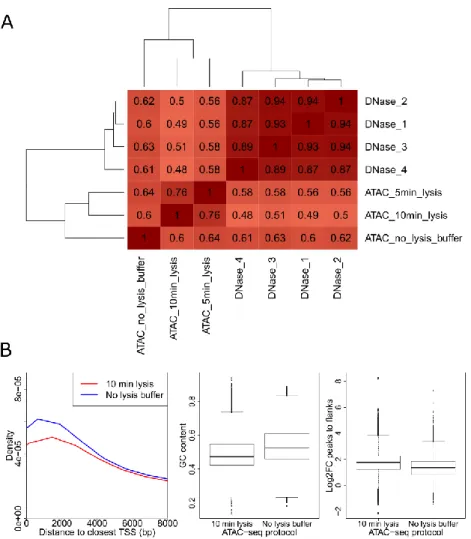
4.1.1. A modified ATAC-seq protocol decreases mtDNA contamination and improves agreement with DNase-seq ... 38
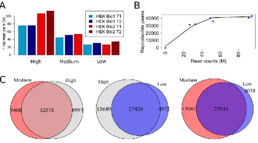
4.1.2. Open chromatin regions are found reliably at moderate library depths ... 41
4.1.3. Sequence bias of ATAC-seq deviates from that of DNase-seq ... 44
4.1.4. ATAC-seq and DNase-seq generate different footprint shapes for the same factor ... 45
4.1.5. Footprinting using ATAC-seq and DNase-seq uncovers common bound sites ... 46
4.1.6. Number of reproducible footprints scales with library depth ... 49
4.1.7. Properties of footprinting apply to larger sets of transcription factors... 49
4.1.8. Protocol-specific sequence biases influence footprinting efficiency ... 52
4.2. Part 2: Characterization of tissue-specific cis-regulatory elements in Drosophila embryonic development ... 56
4.2.1. Nuclear sorting coupled to ATAC-seq or DNase-seq captures tissue-specific cis-regulatory elements ... 56
4.2.2. Cis-regulatory elements open in the same tissue-specific context share common sequence signatures ... 58
4.2.3. Contrasting regions open in the same tissue at consecutive time-points uncovers temporally resolved sequence features... 62
4.2.4. Transcription factor footprinting poses challenges in this system ... 65
4.2.5. An integrative model allows finding putative binding sites for a multitude of factors ... 70
5. Discussion ... 72
Appendix A: Supplementary tables (part 1) ... 76
Appendix B: Supplementary tables (part 2) ... 80
References ... 95
Acknowledgements ... 104
iii Table of Figures
Figure 1: Transcriptional regulation of gene expression...6
Figure 2: Expression of five main mesoderm TFs during early embryonic development...8
Figure 3: The developing CNS and the three columns of the neuroectoderm…...9
Figure 4: Illumina/Solexa sequencing chemistry...11
Figure 5: ChIP-seq...12
Figure 6: BiTS-ChIP protocol...14
Figure 7: DNase-seq...16
Figure 8: ATAC-seq…...17
Figure 9: ChIP-seq peak calling...20
Figure 10: A position weight matrix and its motif logo visualization...22
Figure 11: Generating ATAC-seq libraries without the usage of lysis buffer increases agreement with DNase-seq...39
Figure 12: Characterization of ATAC-seq datasets generated with different protocols in K562 cells....40
Figure 13: The task of finding open chromatin regions saturates at medium depth...41
Figure 14: Pairwise Pearson correlations of read counts in 100bp bins genome-wide for the ATAC-seq and DNase-seq datasets in HEK293 cells...42
Figure 15: Analysis of reproducible peaks in HEK293 cells...43
Figure 16: Library complexity and saturation plots for HEK293 ATAC-seq datasets...44
Figure 17: The sequence bias of the Tn5 transposase is distinct from that of DNase I...45
Figure 18: The number of reproducible footprints scales with library depth...47
Figure 19: Performance of footprint models trained in HEK293 DNase-seq and ATAC-seq datasets....48
Figure 20: The relevance of the learned footprint models...51
Figure 21: Analysis of NRF1 footprints...52
Figure 22: TF-footprinting accuracy is linked to clear discrimination of footprint from background...54
Figure 23: Method and TF-specific footprinting efficiency...55
Figure 24: Tissue- and time-point-specific DNase-seq signal profiles around Mef2 gene locus...57
Figure 25: Tissue- and time-point-specific ATAC-seq signal profiles around ind gene locus...58
Figure 26: Motif enrichment results in tissue-specific DHSs...60
Figure 27: Overlaps between enriched motifs and GKM-SVM-derived PWMs...62
Figure 28: Motif enrichment results in time-point-specific DHSs...64
Figure 29: Differences in DNase I cut profiles and footprinting in native and crosslinked S2 DNase-seq data...66
Figure 30: DNase I cut profiles around motif sites of 5 mesoderm specific TFs...68
Figure 31: Performance of footprint models compared to ranking by tag counts...68
Figure 32: Motif enrichment and footprinting analyses in ATAC-seq data...70
Figure 33: A logistic regression with three features is highly predictive of TF binding...71
iv
Erklärung
Hiermit erkläre ich, die Dissertation selbstständig und nur unter Verwendung der angegebenen Hilfen und Hilfsmittel angefertigt zu haben. Ich habe mich anderwärts nicht um einen Doktorgrad beworben und besitze keinen entsprechenden Doktorgrad. Ich erkläre, dass ich die Dissertation oder Teile davon nicht bereits bei einer anderen wissenschaftlichen Einrichtung eingereicht habe und dass sie dort weder angenommen noch abgelehnt wurde. Ich erkläre die Kenntnisnahme der dem Verfahren zugrunde liegenden Promotionsordnung der Lebenswissenschaftlichen Fakultät der Humboldt-Universität zu Berlin vom 5. März 2015.
Weiterhin erkläre ich, dass keine Zusammenarbeit mit gewerblichen Promotionsberaterinnen/Promotionsberatern stattgefunden hat und dass die Grundsätze der Humboldt-Universität zu Berlin zur Sicherung guter wissenschaftlicher Praxis eingehalten wurden.
Berlin, den
Aslihan Karabacak Calviello
v
Abstract
Cis-regulatory elements such as promoters and enhancers, that govern transcriptional gene regulation, reside in regions of open chromatin. DNase-seq and ATAC-seq are broadly used methods to assay open chromatin regions genome-wide. The single nucleotide resolution of DNase-seq has been further exploited to infer transcription factor binding sites (TFBS) in regulatory regions through TF footprinting. However, recent studies have demonstrated the sequence bias of DNase I and its adverse effects on footprinting efficiency. Furthermore, footprinting and the impact of sequence bias have not been extensively studied for ATAC-seq.
In this thesis, I undertake a systematic comparison of the two methods and show that a modification to the ATAC-seq protocol increases its yield and its agreement with DNase-seq data from the same cell line. I demonstrate that the two methods have distinct sequence biases and correct for these protocol-specific biases when performing footprinting. The impact of bias correction on footprinting performance is greater for DNase-seq than for ATAC-seq, and footprinting with DNase-seq leads to better performance in our datasets. Despite these differences, I show that integrating replicate experiments allows the inference of high-quality footprints, with substantial agreement between the two techniques.
These techniques are further employed to characterize the cis-regulatory elements governing the embryogenesis of a complex organism, the fruit fly Drosophila melanogaster. Combining tight staging of embryos and tissue-specific nuclear sorting with open chromatin profiling, enables the definition of temporally and tissue-specifically resolved putative cis-regulatory elements. Large scale motif enrichment analyses of these elements confirm known associations between TFs and specific tissues or developmental time-points, as well as implicating novel links. Finally, DNase-seq signal and sequence features associated with putative TFBSs are combined in an integrative model that is highly predictive of tissue-specific TF binding.
Taken together, these analyses demonstrate the power of open chromatin profiling and computational analysis in elucidating the mechanisms of transcriptional gene regulation.
vi
Zusammenfassung
Cis-regulatorische Elemente wie Promotoren und Enhancer, die die Regulation der Transkription von Genen steuern, befinden sich in Regionen des dekondensierten Chromatins.
DNase-seq und ATAC-seq sind weit verbreitete Verfahren, um solche offenen Chromatinregionen genomweit zu untersuchen. Die einzel-Nukleotid-Auflösung von DNase- seq wurde des Weiteren genutzt, um Transkriptionsfaktor-Bindungsstellen (TFBS) in regulatorischen Regionen durch TF-Footprinting zu bestimmen. Kürzlich durchgeführte Studien haben jedoch gezeigt, dass DNase I einen Sequenzbias aufweist, welcher nachteilige Auswirkungen auf die Footprinting-Effizienz hat. Auch wurden das Footprinting und die Auswirkungen des Sequenzbias auf ATAC-seq noch nicht umfassend untersucht.
In dieser Arbeit nehme ich einen systematischen Vergleich der beiden Methoden vor und zeige, dass eine Modifikation des ATAC-seq-Protokolls die Ausbeute und die Übereinstimmung mit den DNase-seq-Daten derselben Zelllinie erhöht. Ferner zeige ich, dass die beiden Methoden unterschiedliche Sequenzbiases haben und korrigiere diese protokollspezifischen Biases beim Footprinting. Der Einfluss von Bias-Korrekturen der Footprinting Ergebnisse ist für DNase- seq größer als für ATAC-seq, und Footprinting mit DNase-seq führt zu besseren Ergebnissen in unserer Datensätze. Trotz dieser Unterschiede zeige ich, dass die Integration replizierter Experimente die Ableitung von qualitativ hochwertigen Footprints ermöglicht, wobei die beiden Techniken weitgehend übereinstimmen.
Diese Techniken werden ferner eingesetzt, um die cis-regulatorischen Elemente zu charakterisieren, die die Embryogenese der Fruchtfliege Drosophila melanogaster bestimmen.
Durch die Verwendung von Embryonen die sich im richtigen Entwicklungsstadium befinden, sowie gewebespezifischer Kernsortierung mit offenem Chromatin-Profiling können zeitlich und gewebespezifisch aufgelöste vermeintliche cis-regulatorische Elemente definiert werden.
Umfangreiche Motivanreicherungsanalysen dieser Elemente bestätigen bekannte Zusammenhänge zwischen TFs und spezifischen Geweben oder Entwicklungszeitpunkten und implizieren neue Verbindungen. Schließlich werden DNase-seq-Signal und Sequenzmerkmale, die mit mutmaßlichen TFBSs verbunden sind, in einem integrativen Modell kombiniert, das die gewebespezifische TF-Bindung in hohem Maße vorhersagt.
Zusammengenommen demonstrieren diese Analysen die Fähigkeit der offenen Chromatin- Profilierung und der Computeranalyse zur Aufklärung der Mechanismen der Genregulation.
1. Introduction | 1.1 Thesis outline
1
1. Introduction
The orchestrated regulation of the activity of thousands of protein-coding genes is a fundamental feature of all living organisms, allowing for the maintenance of internal homeostasis and reaction to environmental stimuli. Coordinated gene expression across different cells further allows for organismal development, in which a zygote develops into an embryo containing dozens of different cell types with specialized functions.
While almost all cells of an organism share the same genomic DNA, not all elements in the genome are simultaneously used in all cells; temporal and spatial patterns of gene expression driven by temporally and spatially active cis-regulatory elements (CREs), shape organismal development and cell function. Such specificity is achieved by keeping different portions of the genome accessible in different conditions, facilitated by the organization of DNA around protein macromolecular complexes called nucleosomes, leading to chromatin formation. When accessible (or synonymously: residing in regions of open chromatin), CREs like promoters and enhancers can be bound by regulators such as transcription factors, which in turn are able to tune the transcription levels of target genes. Profiling tens of thousands of accessible regions in chromatin is thus crucial to understanding transcriptional regulation.
Two major experimental methods, DNase-seq and ATAC-seq, couple open chromatin profiling with next-generation sequencing to probe accessible regions genome-wide and have been instrumental in characterizing CREs in multiple organisms. In addition, these techniques harbor the potential to infer the binding of individual transcription factors within open chromatin regions, requiring tailored data analysis methods known as transcription factor footprinting approaches and a thorough understanding of experimental artifacts influencing the results.
Combining the power of open chromatin profiling techniques with established model organisms (such as Drosophila melanogaster) allows for detailed investigation of transcriptional regulatory networks, where both spatial and temporal patterns of promoter and enhancer activities are able shape the precise development of an entire organism.
2 1.1 Thesis outline
In Chapter 2, I present background regarding the molecular biology of transcription (Section 2.1), with a focus on chromatin structure, sequence elements and a short introduction to transcription factors. A brief description of Drosophila early embryo development is then presented in Section 2.2.
Section 2.3 details the experimental techniques used throughout this thesis, with an emphasis on ATAC-seq and DNase-seq. Computational analysis strategies are presented in Chapter 2.4, with a detailed discussion on methods used to infer transcription factor binding in open chromatin regions.
Chapter 3 contains a detailed description of the experimental and analytical methods used in this thesis, relating to experiments performed on human and Drosophila cells.
Results are presented in Chapter 4; in Section 4.1, I present results on comparing ATAC-seq and DNase-seq with respect to their ability in detecting open regions, using data from human cell lines. Inference of transcription factor binding using footprinting is presented, outlining the experimental biases affecting the two techniques. Different transcription factors show distinct footprint and background signal profiles in ATAC-seq and DNase-seq, where footprinting performance depends on the intrinsic experimental biases of the two techniques, in a protocol- and transcription factor-specific manner. Integrating information from biological replicates is presented as a strategy to infer high-confidence, reproducible transcription factor footprints in open chromatin.
Section 4.2 covers results associated with the application of open chromatin profiling in the early embryonic development of the fruit fly Drosophila melanogaster. Open chromatin is profiled for specific tissue subsets within precisely staged embryos (performed by the laboratories of Prof. Eileen Furlong at the EMBL and Dr. Robert Zinzen at the MDC), enabling the inference of both tissue- and time point-specific putative CREs. Different analysis strategies uncover the rich sequence content, including transcription factor binding motifs, underlying these regions. These analyses link transcription factors to putative CREs that are spatially and temporally active in neural and mesoderm development, finding known associations as well as implicating novel ones.
Section 5 includes a brief discussion, where I discuss the results presented in Chapter 4 and highlight the potential advantages and shortcomings of my work in the broader context of
1. Introduction | 1.1 Thesis outline
3
transcription factor binding and motif inference. Appendix and reference sections can be found at the end of the thesis.
4
2. Background
2.1. Transcriptional regulation of gene expression 2.1.1. Chromatin
In eukaryotic cells, nuclear DNA is assembled into a higher order structure, known as chromatin. Chromatin consists of a basic repeating unit named the nucleosome, which is an octamer made up of two copies each of histones H2A, H2B, H3 and H4 around which 147 base pairs (bp) of DNA is wrapped1. These histones are termed “core histones” and they consist of two domains: a “histone-fold” motif which is responsible for histone-histone and histone-DNA interactions, and an amino-terminal tail which can be subjected to posttranslational modifications (PTMs)2. The nucleosomes were found to be separated by 10-60 bp of linker DNA; the organization of this 10 nm chromatin fiber is termed the “nucleosomal array” or the primary structural unit3. Nucleosome-nucleosome interactions constitute the 30 nm fiber, also known as the secondary structural unit which is mediated by the linker histones such as H1 and H5 and further compaction of this 30 nm fibre forms the tertiary structural unit, resulting in the 240 nm metaphase chromosome seen in mitosis3.
Two distinct chromatin structures were found via carmine acetic-acid staining of interphase nuclei4. The densely stained regions were found to maintain their condensed state throughout the cell cycle and these regions were collectively named “heterochromatin”. Other regions (lightly stained in interphase) were observed to decondense as the cells progressed from metaphase to interphase; these were later found to exist in the form of the 30 nm fiber at this stage of the cell cycle5 and these regions were termed “euchromatin”.
Euchromatin is generally defined as early replicating in S phase, gene rich and transcriptionally permissive; whereas heterochromatin is late replicating in S-phase, gene-poor, transcriptionally inactive in general, low in recombination activity and associated with repeat sequences abundant in pericentric and telomeric regions6. Chromatin modifications were found to be associated with these different chromatin states, for example DNA methylation is abundant in heterochromatin whereas DNA in euchromatin is generally hypomethylated7. Many histone PTMs have also been characterised to date (acetylation, methylation, phosphorylation, ubiquitylation, sumoylation, ADP ribosylation, deimination and protein isomerisation) which are associated with heterochromatin or euchromatin, depending on the site of modification2. Regulation of chromatin structure, via the action of these modifications, or other chromatin-
2. Background | 2.1. Transcriptional regulation of gene expression
5
associated proteins, play crucial roles in the transcriptional regulation of gene expression, as explored in the next sections.
2.1.2. Cis-regulatory elements
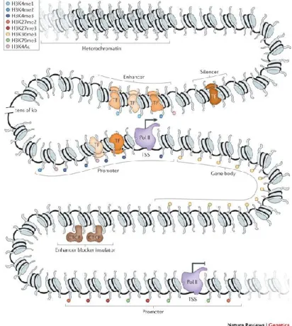
Transcriptional regulation of gene expression is mediated by the collective action of cis- regulatory elements (CREs) such as promoters, enhancers, silencers and insulators (figure 1).
At a basal level, gene transcription is achieved by the assembly of the transcription preinitiation complex (PIC), which is comprised of RNA polymerase II (Pol II, enzyme catalyzing transcription) and the basal transcription factors, at the core promoter regions8. The core promoter regions, which refer to the 50-100bp regions surrounding transcription start sites (TSSs), have two main classes: peaked (TSS spanning at most several nucleotides) and broad (several weak TSSs over an extended region)9. Core promoters are rich in sequence content and contain numerous motifs such as the TATA box, BRE, Inr, MTE, DPE, DCE, and XCPE1, some of which constitute binding sites for basal transcription factors, and the prevalence of which depends on the promoter class9. Enhancers, on the other hand, are TSS-distal elements that regulate expression by interacting specifically with promoters via looping10. These distal elements are bound by transcription factors (TFs, see next section), which in turn recruit coactivators/corepressors that regulate the target gene10.
6
Figure 1: Transcriptional regulation of gene expression. Cis-regulatory elements (promoter, enhancer, silencer, insulator) are schematically shown around a gene locus. Factors and histone modifications associated
with these elements are also shown. Adapted from reference11.
Transcriptional gene regulation by these elements is closely linked to chromatin regulation, as active promoters and enhancers are found in open chromatin regions, where nucleosomes are locally displaced10. Therefore, locations of cis-regulatory elements can be assayed via open chromatin profiling techniques such as DNase-seq and ATAC-seq (see section 2.3.3). In accordance with this, active elements harbor active histone marks such as histone H3 lysine 4 trimethylation (H3K4me3) for promoters and H3K4me1 and H3K27 acetylation (H3K27ac) for enhancers2. Chromatin accessibility enables the binding of tissue-specific TFs to their cognate sequences (see next section).
2. Background | 2.2. Drosophila melanogaster as a model organism of embryogenesis
7 2.1.3. Transcription factors
As mentioned above, TFs bound at short specific sequences called motifs (see section 2.4.3.1) within CREs are major regulators of gene expression12. TFs may be activators or repressors of gene expression and in most cases many factors act together to exert combinatorial control12. There are multiple mechanisms that affect factor binding, such as the affinity to target sequences and the number and arrangement of sites with respect to each other13. In addition, while pioneer transcription factors can bind nucleosome-associated inaccessible DNA and make the local chromatin structure more accessible by displacing nucleosomes, binding of other transcription factors require an already open/primed structure14. Many TFs bind enhancers in a tissue and time-point specific manner, and some act as master regulators that specify a given lineage12.
TFs are classified according to their families, which in turn is based upon their specific DNA- binding domains (DBDs)15. There are around 100 characterized eukaryotic DBDs to date, examples of which include helix-turn-helix (HTH), homeodomain, zinc finger (ZF), leucine zipper (bZIP) and helix-loop-helix (bHLH)15. The motifs recognized by TFs are influenced by the specific interactions between the DBD and the underlying DNA sequence.
2.2. Drosophila melanogaster as a model organism of embryogenesis
Drosophila melanogaster is a widely studied model organism, and consequently the stages of embryonic development are well documented. At the onset of fertilization, a set of maternally deposited and localized factors, namely bicoid, nanos and torso, lead to patterning in the developing embryo, by forming gradients and activating zygotic gap genes, which in turn activate pair-rule genes16. This occurs within the first three hours of embryogenesis, where 13 rapid rounds of mitotic division takes place, without membrane formation, and the 6000 nuclei sharing the same cytoplasm17. This constitutes the blastoderm stage (stage 5), followed by gastrulation (stage 8), and time-points spanning 2-4hr post fertilization (pf) correspond to these stages. Upon gastrulation, the three germ layers (ectoderm, endoderm and mesoderm) are generated. As the datasets analyzed in this thesis are focused on the mesoderm and neurogenic ectoderm, the next stages will be summarized for these germ layers.
8 2.2.1. Specification of the mesoderm
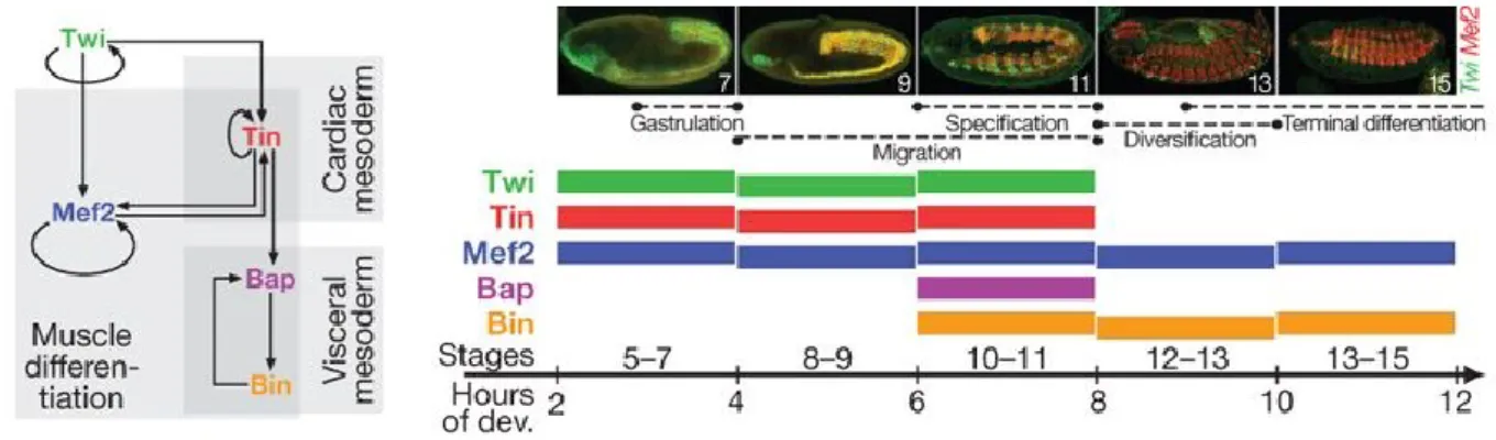
The mesoderm gives rise to the somatic, visceral and heart muscle18. In the developing mesoderm, 2hr windows post fertilization correspond to the following stages: 4-6hr pf (stages 8-9) multipotent mesoderm, 6-8hr pf (stages 10-11) specification, 8-10hr pf (stages 12-13) diversification and 10-12hr pf (stages 13-15) terminal differentiation19 (figure 2). The TF twist has a central role in mesoderm specification at multiple stages, starting as early as gastrulation18. It also regulates other central mesoderm-specific genes dMef2, which primes the differentiation into muscle20, and tinman, which specifies the dorsal mesoderm21. Tinman further regulates bagpipe, which, in conjunction with biniou, specifies the visceral mesoderm22 (figure 2). These TFs constitute the master regulators of mesoderm specification19.
Figure 2: Expression of five main mesoderm TFs during early embryonic development. Regulatory relationships between the 5 TFs is shown on the left. Stage specific expression patterns of twi and mef2 in the
developing embryo is shown on the right panel (above), with the embryonic development stages (in 2hr windows) in which all 5 TFs are expressed, are stated below. Adapted from reference19.
2.2.2. Specification of the neurogenic ectoderm
The neurogenic ectoderm gives rise to the central nervous system. In the developing neurogenic ectoderm, 2hr windows post fertilization correspond to the following stages: 4-6hr pf neuroblast formation, 6-8hr pf newborn neurons, 8-10hr pf neural patterning and 10-12hr pf terminal differentiation. The neurogenic ectoderm is made up of three columns along the dorsoventral (DV) axis: ventral, intermediate, and dorsal, where the cell fates for these columns are specified by the homeobox genes, vnd, ind, and msh, respectively23. Figure 3 shows the respective locations of the three columns in the developing embryo, marked by the expression of these genes. Proneural genes achaete, scute, lethal of scute, wingless, hedgehog, gooseberry, and engrailed also play important roles in neuroblast formation23.
2. Background | 2.3. Genome-wide sequencing techniques to identify and characterize cis-regulatory elements
9
Figure 3: The developing CNS and the three columns of the neuroectoderm. The CNS development in embryos at stages 5, 8 and 9, is shown (the neurogenic region shown in light purple, left). The three columns of
the neuroectoderm, as marked by vnd, ind and msh, are shown (together with segment polarity and pair rule genes that define segment boundaries, right). Adapted from http://www.sdbonline.org and reference24.
2.3. Genome-wide sequencing techniques to identify and characterize cis-regulatory elements
2.3.1. Next-generation sequencing
Before the advent of next-generation sequencing technologies, the predominant methods for uncovering the sequence of DNA fragments have been Maxam-Gilbert25 and Sanger sequencing26. Maxam-Gilbert method uses a set of chemical reactions that cleave a DNA template preferentially at one or two specific nucleotides (G+A, G, C+T, C). On the other hand, Sanger sequencing takes advantage of nucleotide analogues (dideoxynucleotides) that terminate the elongation of a template DNA molecule by DNA polymerase at a specific nucleotide (A, C, G or T). For both methods, conducting all four respective reactions on the same template and visualizing the resulting fragments side by side via gel electrophoresis, allows decoding the template sequence. Even though protocol modifications such as labeling the four reactions with different fluorophores to have direct fluorescent readout has increased automation in the case of Sanger sequencing27,28, these methods have limited throughput. For instance, the human genome projects29,30, where Sanger sequencing was employed, have been collective efforts of multiple groups, over the course of several years, with an estimated cost of 0.5-1 billion dollars31. Around the time the human genome projects were approaching completion, the National Human Genome Research Institute started an advanced DNA sequencing technology program, to fund the development of new technologies aimed at sequencing an individual human genome for 1000 dollars or less32. This set the stage for many
10
next-generation sequencing technologies, including Illumina/Solexa that has been used in the generation of all datasets analyzed in this thesis.
The first step of the Illumina/Solexa sequencing workflow is library preparation33. In general, this involves DNA fragmentation, forward and reverse adapter ligation to the ends of the resulting fragments and amplification via PCR, although the experimental details depend on the protocol and starting material. For instance, RNA molecules need to be reverse transcribed into cDNA first. The following steps are cluster generation and sequencing, as illustrated in Figure 4. Cluster generation is achieved by a process called solid-phase amplification. This process starts with the adapter-ligated fragments annealing to complementary oligonucleotides covalently attached to the surface of a glass slide, known as the flow cell. The annealed oligonucleotides prime an extension reaction copying the original strand, creating flow cell- bound fragments. In turn, the free ends of the bound fragments anneal to other nearby complementary oligonucleotides, forming bridges. This initiates further rounds of extension and annealing (e.g. bridge amplification), generating many copies of the same fragment locally, called a cluster. All clusters on the flow cell are then sequenced via a reversible termination strategy. Sequencing primer anneals uniquely to the forward adapter and primes the extension reaction. Akin to Sanger sequencing, elongation-terminating nucleotide analogues are used. In contrast to the dideoxynucleotides used in Sanger sequencing, however, the fluorescently labeled 3´-O-azidomethyldNTPs used in this reaction enable the termination to be reversed34. In each round, the correct base is incorporated into the growing chain, visualized via the fluorescent signal and the termination reversed for the next base to be added. Cycles are repeated until the desired sequence length (e.g. read length) is achieved. In this way, sequences from one end of the fragments are uncovered, termed single-end sequencing. Both ends can be sequenced by repeating the whole process with a second sequencing primer complementary to the reverse adapter, termed paired-end sequencing.
2. Background | 2.3. Genome-wide sequencing techniques to identify and characterize cis-regulatory elements
11
Figure 4: Illumina/Solexa sequencing chemistry. Fragments are subjected to bridge amplification followed by cluster generation (left). Fragments are then sequenced via a cyclic reversible termination strategy (right).
Adapted from reference35.
Of the sequencers produced by Illumina, the HiSeq series and NextSeq 500 have been used in the production of the datasets analyzed in this thesis. To put the throughput into context, both HiSeq 2500 and NextSeq 500 machines can produce reads from a human genome at 30x coverage, in less than 30 hours31. This paves the way to probe the genome at unprecedented scale, using a multitude of genomics techniques.
2.3.2. Techniques to profile transcription factor binding sites and histone modifications Transcription factors and histone modifications play crucial roles in the transcriptional regulation of gene expression. Therefore, techniques that enable them to be mapped genome- wide, have become instrumental in probing the complex transcriptional programs of cells.
12 2.3.2.1. ChIP-seq
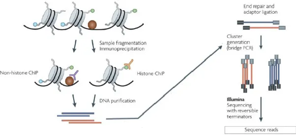
Chromatin immunoprecipitation (ChIP) is perhaps the most widely used method to profile in vivo protein-DNA interactions36,37. In ChIP, proteins are covalently crosslinked to DNA using formaldehyde, to stabilize existing contacts36,38. The cells and nuclei are lysed, and the chromatin is then sheared by sonication to obtain shorter fragments, ideally in the 200-500 base pair range (Figure 5). Next, fragments bound to the protein of interest are enriched using an antibody specific to the protein (eg. the immunoprecipitation step). The DNA fragments are released from the protein-DNA complexes, by reversing the crosslinks. Finally, fragment sequences are determined to infer the binding locations of the protein of interest. In the early days of the ChIP assay, this was mostly achieved by designing probes specific to a locus of interest and assessing whether the probes hybridized to the obtained fragments36,37. Another method readily used is quantitative real-time polymerase chain reaction (qPCR) with primers against regions of interest38. Both approaches are low-throughput as they require pre-selection of candidate regions. Combining ChIP with next generation sequencing (ChIP-seq), overcomes this issue and profiles chromatin-associated proteins at a genome-wide scale.
Figure 5: ChIP-seq. In ChIP chromatin is fixed, fragmented, and enriched for the bound protein or histone modification of interest by immunoprecipitation with a specific antibody (left). Adapters are ligated and libraries
are sequenced (right). Adapted from reference39.
In ChIP-seq, adapters are ligated to the ends of the fragments, followed by cluster generation and sequencing steps, as detailed in the previous section (Figure 5). In this way, millions of fragments can be sequenced in parallel. An important control in ChIP-seq is the input or total DNA, obtained by processing the samples in the same way, but omitting the
2. Background | 2.3. Genome-wide sequencing techniques to identify and characterize cis-regulatory elements
13
immunoprecipitation step38. Input DNA is sequenced alongside the immunoprecipitated samples and gives insights into the fragmentation and sequencing biases. An additional control used in some cases is immunoprecipitation with a non-specific antibody (eg. IgG)38.
Since the first ChIP-seq studies published in 200740–43, there have been many variations to the protocol44. For instance, nano-ChIP-seq45 and linear DNA amplification (LinDA)46 are two variations that require much less starting material than the original protocol: ~10000 cells as opposed to ~10 million. In another variation, ChIP-exo47, the immunoprecipitated fragments are subjected to 5’ to 3’ exonuclease digestion, which brings the 5’ ends of the fragments to the immediate vicinity of the bound protein, increasing the resolution from ~200 base pairs of the standard protocol to pinpointing the binding site. The next section will focus on batch isolation of tissue-specific chromatin for immunoprecipitation (BiTS-ChIP)48, another technique that extends the standard ChIP-seq protocol and which has been partially used in the generation of some of the datasets analyzed in this thesis.
2.3.2.2. BiTS-ChIP
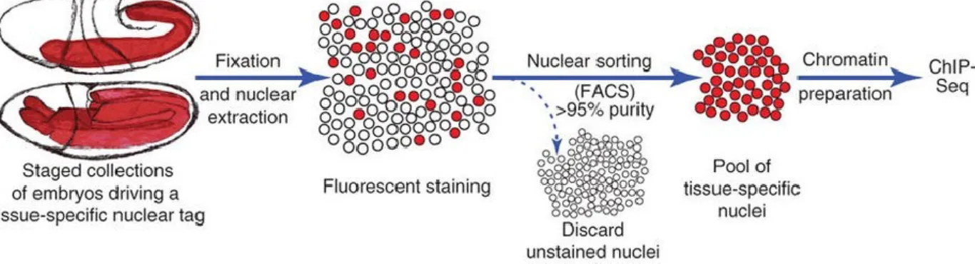
BiTS-ChIP48,49 allows conducting ChIP-seq on a batch of tissue-specific nuclei isolated from a developing embryo (figure 6). The first step is to find a nuclear marker that is expressed exclusively in the tissue of interest and that can be used for fluorescent labeling of the nuclei.
This can either be an endogenous protein or a transgene driven using a tissue-specific enhancer, coding for a tagged nuclear protein. Embryos expressing such a nuclear marker are collected, staged (eg. aged to the developmental stage of interest) and formaldehyde fixed to stabilize existing protein-DNA contacts. Individual nuclei are extracted by mechanical disruption of the fixed embryo. The nuclei are then fluorescently labeled by staining using a highly specific antibody against the chosen nuclear marker. Antibody staining is not needed if the nuclear marker is designed to have a fluorescent tag. Subsequently, a highly pure (typically >97%) population of fluorescently labeled, tissue-specific nuclei is obtained by fluorescence activated cell sorting (FACS). These nuclei are used in ChIP-seq experiments to infer tissue-specific patterns of histone modifications or binding of transcription factors and other chromatin- associated proteins.
14
Figure 6: BiTS-ChIP protocol. Embryos expressing a tissue-specific nuclear marker are aged to the desired stage and formaldehyde fixed, followed by nuclear extraction, staining and FACS sorting. This results in a pool
of tissue-specific nuclei that can then be assayed by ChIP-seq. Adapted from reference49.
2.3.3. Techniques to profile open chromatin
As covered in section 2.1.2, tissue- and developmental stage-specific regulatory elements reside in nucleosome-free, accessible regions of the genome. These regions are hypersensitive to nuclease attack50. Digestion with the nuclease DNase I, coupled to high throughput sequencing (DNase-seq), is the first established genome-wide technique to probe such open chromatin regions51,52, and is widely applied in research consortia such as ENCODE53,54 or the Roadmap Epigenomics55.
2.3.3.1. DNase-seq
Initially isolated from bovine pancreas56, DNase I is a nuclease that can cleave DNA molecules by hydrolyzing the phosphodiester bonds of the sugar phosphate backbone57. In the mid-70s, studies have demonstrated that DNase I preferentially cleaves transcriptionally active chromatin58,59. Specifically, cells where selected gene loci (globin58 and ovalbumin59) are transcriptionally active, are subjected to digestion by DNase I. The resulting DNA is observed to be depleted for fragments associated with the active genes, as shown by decreased annealing to gene-specific probes. This effect is not observed for cells where the genes are not transcribed, leading to the hypothesis that transcriptional activity is associated with an altered chromatin conformation, more susceptible to DNase I cleavage. These observations were extended some years later, in studies of Simian Virus 4060 and Drosophila chromatin61, which demonstrated that DNase I cleaves the underlying chromatin in a position-specific manner. These studies estimated two regions preferably digested by DNase I to be shorter than the length of DNA
2. Background | 2.3. Genome-wide sequencing techniques to identify and characterize cis-regulatory elements
15
wrapped around 2 nucleosomes60, and approximately 140 base pairs61, respectively.
Furthermore, both studies discussed that these regions could possibly be devoid of nucleosomes. They were defining for the first time, what we now know to be DNase hypersensitive sites (DHSs).
Historically, DHSs were mapped using a method called indirect end-labeling62–64. Briefly, the chromatin is first digested by DNase I, and then the isolated DNA cleaved further by a rare- cutting sequence-specific restriction endonuclease (RE). The resulting fragments are separated by gel electrophoresis, transferred to a membrane and hybridized to probes specific to the immediate flanks of the RE cut sites. The determined fragment lengths provide a direct measure of the distance between the RE and DNase I cleavage sites, from which the DHSs can be inferred. This method is low-throughput and can only be applied to a limited number of loci at a time, as it requires the loci of interest to be previously characterized (eg. knowledge of sequence and RE recognition sites). In contrast, DHSs are readily mapped today with the high- throughput, genome-wide DNase-seq method.
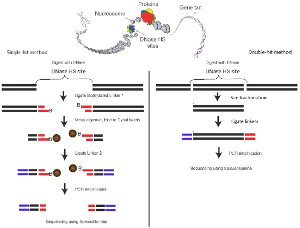
There are two variations of DNase-seq that are generally referred to as single-hit51,65 and double-hit52 protocols, as the resulting fragments represent a DNase I cut on one or both ends, respectively. In the single-hit protocol (figure 7, left), DNase I digestion is carried out and the first linker harboring an MmeI restriction enzyme recognition site is ligated to the digested ends. MmeI then cuts 20bp downstream from its recognition site, where the second linker is subsequently ligated. In the double-hit protocol (figure 7, right), the DNase I digested chromatin is subjected to size fractionation to get 100-500bp fragments. Illumina adapters are then ligated to the ends of the fragments. In both protocols, the linker-flanked fragments are PCR amplified, purified and sequenced according to the Illumina sequencing workflow.
Computational analysis of DNase-seq datasets to infer DHSs and transcription factor footprints are discussed in sections 2.4.2 and 2.4.3.
16
Figure 7: DNase-seq. In the single-hit DNase-seq protocol, a 20bp region representing one end of a DNase I- cut fragment is retrieved via an MmeI digestion step (left). In the double-hit protocol, the fragments are cleaved
on both ends by DNase I (right). Adapted from reference65.
2.3.3.2. ATAC-seq
A more recent technique to profile open chromatin regions is the assay for transposase- accessible chromatin using sequencing (ATAC-seq)66. Instead of a nuclease like DNase I, ATAC-seq employs Tn5 transposase enzymes. Transposases contribute to genomic rearrangements and consequently genome evolution, by mobilizing DNA elements called transposons67. Tn5 is a bacterial transposon normally functioning to confer antibiotic resistance to the host, through the three resistance genes it harbors (kanamycin, bleomycin and streptomycin)68,69. As with many others, mobilization of the Tn5 transposon is realized via a
“cut-and-paste” mechanism where it is cleaved from its original location and inserted into the target DNA by the Tn5 transposase69. This depends on the specific interaction of the transposase with the 19bp sequences at the two ends of the Tn5 transposon. The Tn5 transposon-transposase complex then binds the target DNA and via a nucleophilic attack, the 3’ ends of the transposon get covalently linked to the 5’ ends of the cleaved target DNA70. During this process, the minus strand of the target DNA is cleaved at a position 9bps
2. Background | 2.3. Genome-wide sequencing techniques to identify and characterize cis-regulatory elements
17
downstream of the plus strand, which leads to the duplication of these 9bps on either side of the inserted transposon. A better understanding of and modifications to the components of this system, led to its usage as an in vitro tool70. These include making the Tn5 transposase hyperactive through mutations71, and using a modified version of the 19bp end sequence called the mosaic end (ME) with greater transposition efficiency72. Furthermore, it was found that pre-loading hyperactive Tn5 transposases in vitro with sequencing adapters harboring ME sequences, without the intervening transposon DNA, is sufficient for transposition73,74. Since there is no intervening DNA, this altered transposition reaction leads to the fragmentation of target DNA via transposase attack and cleavage while the resulting fragments are simultaneously tagged by adapter ligation to the 5’ ends, a process known as “tagmentation”74. These developments and the reports of transposons preferentially integrating into nucleosome- free regions75, set the stage for ATAC-seq as a Tn5 transposase-based method to profile open chromatin66. ATAC-seq has a fast and straightforward protocol that comprises of cell/nuclei isolation, lysis, tagmentation, PCR amplification and sequencing (figure 8). Much less starting material is required for ATAC-seq in comparison to DNase-seq, ~500-50,00066 vs ~1-10 million65 cells or nuclei, respectively, although recent protocol variations allow both techniques to be applied at the single cell level76–78. As for DNase-seq, computational analysis of ATAC- seq datasets are discussed in more detail in sections 2.4.2 and 2.4.3.
Figure 8: ATAC-seq. In ATAC-seq, Tn5 transposase dimers insert adapters into open chromatin regions, generating sequencing-ready fragments. Adapted from reference66.
18
2.4. Computational analysis of genome-wide sequencing datasets 2.4.1. Read processing, alignment and filtering
As described in section 2.3.1, next generation sequencing technologies output sequences of defined length, also known as reads, belonging to fragments of interest from a given experimental setup. The output at this stage is generally in fastq format, which includes both the sequence information, as well as a per nucleotide quality metric for each read. A popular choice for the quality metric is called the phred score79, which is essentially a measure of the probability of the base call during sequencing being correct for each nucleotide.
As adapters are ligated to the fragments for sequencing (see section 2.3.1), reads may contain adapter sequences which need to be trimmed, since otherwise they would interfere with proper alignment to the reference genome. Adapter sequences and where in the read they might be encountered are specific to the experimental setup and read length. For instance, an ATAC-seq library has a range of fragment lengths, starting from as short as 38bp74. The first nucleotide in the read corresponds to the 5’ end of the fragment. When the read is longer than the fragment, therefore, the 3’ end of the read will comprise of adapter sequences. Another example can be a single-hit DNase-seq library, where the fragment length is 20bp51, and the reads would need to be trimmed down to this length. Tools for adapter trimming, can generally also be used to trim low quality bases from reads when needed.
The next step is to align the reads to the reference genome, in other words to determine which genomic region the read (and fragment) was originally derived from. This is essentially an approximate string matching problem80: the objective is to find where the read sequence matches the reference sequence, while allowing for mismatches and gaps. The main reasons for this are errors in sequencing and differences between the assayed sample and the reference genome due to sequence variation. Another consideration is the sheer amount of data. Aligning millions of reads to a reference genome millions of bases long, requires efficient algorithms.
Two algorithmic ideas used by aligners are filtering and indexing80. Briefly, filtering eliminates regions of the reference genome where a match is not expected for a given read, by comparing the shorter subsequences within the read to the reference genome81. Indexing, on the other hand, refers to preprocessing the reference genome to allow matching sequences to be queried much faster. The main indexing approaches used are the enhanced suffix array82 and the FM- index83, which is based on the Burrows-Wheeler transform84. Aligners Bowtie285 and BWA86,
2. Background | 2.4. Computational analysis of genome-wide sequencing datasets
19
used in the analyses presented in this thesis, incorporate the FM-index. The output is in sam (short for sequence alignment/map) format which can be converted to the binary bam format.
Following the alignment, the .bam file can be further processed as needed. One of the first choices to be made is the handling of multimappers, i.e. reads that map to multiple locations in the genome. These may be filtered out to retain only reads that map uniquely to a single location, which increases certainty at the expense of coverage over repetitive regions. Another consideration is that, most library preparation methods include a PCR amplification step, which can lead to the same fragment to be sequenced multiple times. These PCR duplicates may be removed, with the choice depending on the experimental protocol: if independent fragments originating at the same location are expected, removing duplicates may discard some true fragments. Paired-end sequencing may aid in more confident removal of duplicates, as both 5’
and 3’ ends are considered. The final processed .bam file can then be used in downstream analyses.
2.4.2. Finding regions of enrichment via peak calling
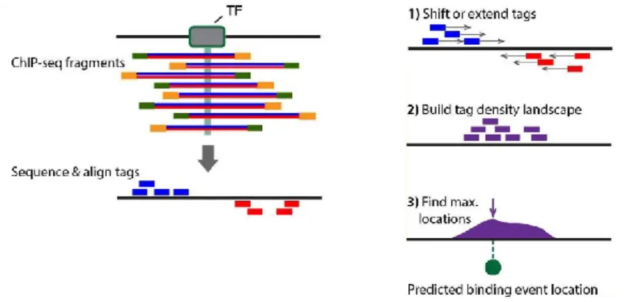
Once discovering where the reads originated from in the reference genome via the alignment step, one common downstream analysis is to find the regions of enrichment, i.e. regions where the reads accumulate to generate enriched signal over background expectation. This is achieved by peak calling algorithms which have slight differences in application depending on the experimental protocol. For instance, in ChIP-seq (see section 2.3.2.1 and figure 5), the fragments of interest encompass a TF or histone modification. The sequenced reads belong to the 5’ ends of these fragments, either on the plus or minus strand, shown as blue and red tags, respectively in figure 9, left. For the tag density to reflect the center of binding, many peak calling tools estimate fragment lengths and subsequently shift or extend the tags in the 3’
direction (figure 9, right)87. The updated signal profile is then used to calculate regions of enrichment that reflect TF binding or locations of modified histones. On the other hand, in DNase-seq and ATAC-seq, the 5’ ends of the reads represent the DNase I cut sites and the Tn5 transposition sites, respectively (see sections 2.3.3.1 and 2.3.3.2). Therefore, in this case peak calling algorithms are used to infer 5’ read end pileups, without shifting. Open chromatin regions, and thus cis-regulatory elements, are inferred in this way.
20
Figure 9: ChIP-seq peak calling. In ChIP-seq, the fragments span binding sites of the factor of interest (left).
The 5’ end of the fragments are shifted or extended to represent the center of binding (right). Adapted from reference87.
The algorithmic approaches utilized by peak callers will be exemplified via two specific tools used in this thesis: MACS88 and JAMM89. For ChIP-seq datasets, MACS estimates the fragment length, d, and shifts all reads by d/2 towards the 3’ direction. To find peaks, MACS models read counts with a Poisson distribution, where mean and variance are expressed with a single parameter, lambda. As covered in section 2.3.2.1, input controls are essential for ChIP- seq experiments. By estimating lambda from the input control locally (i.e. from the same genomic regions as the peak candidates), MACS finds peaks that are significantly enriched over input. JAMM, also estimates the fragment length, d, however instead of shifting reads, it extends them towards the 3’ direction, to match d. JAMM first determines broad windows of enrichment (over the control sample) throughout the genome, and then finds peaks within those windows by clustering the signal. Gaussian mixture models90 with peak and noise components are used to this end. Both MACS and JAMM can be used with ChIP-seq data, as well as with DNase-seq and ATAC-seq data when the parameters are set accordingly.
A common method to find reliable peak sets is called the Irreproducible Discovery Rate (IDR)91. The IDR pipeline is comprised of calling peaks in replicates separately, comparing the results to assess both the extent of overlap among peak sets and the similarity of score ranks among overlapping peaks, and subsequently finding the number of reproducible peaks at a given IDR threshold.
The identified peaks are subject to further downstream analyses depending on the type of experiment. Among these is differential signal analysis, which refers to methods such as EdgeR92 and DESeq93. Initially designed to assay differential gene expression among two
2. Background | 2.4. Computational analysis of genome-wide sequencing datasets
21
conditions, these methods can be employed in any case where regions of interest can be defined (e.g. peaks) and replicates are available for sets of conditions to be compared. In general, read counts within peaks are modeled using the negative binomial distribution, where the parameter for variance separates technical from biological variation, facilitating the identification of regions that show significantly higher signal in one condition compared to the other.
2.4.3. Finding transcription factor binding sites
As the previous section illustrated, peak calling on TF ChIP-seq datasets allows finding TF- bound regions genome-wide. However, this analysis has a relatively low resolution (i.e. the identified regions are much larger than the actual TF-DNA contact sites, 100-200bps vs 6- 15bps, respectively) and would require a separate ChIP-seq experiment to be conducted for each TF of interest. Therefore, in the following sections, approaches to find putative TF binding sites at higher resolution is discussed, first focusing on sequence features defined by position weight matrices, followed by the data-driven TF footprinting.
2.4.3.1. Position weight matrices
TFs bind short (typically 6-15bps) and specific sequences throughout the genome. Individual binding sites of a given TF are not always identical; but display position-specific nucleotide preferences when aggregated, also known as binding motifs94. Motifs are most commonly represented via position weight matrices (PWMs)95. As shown in figure 10, each column in a PWM represents a base position, with the rows giving the weights of each of the four nucleotides at that position. The weights are usually log likelihoods (against a background model) of observing a given nucleotide at a given position, and an equivalent representation with plain probabilities or frequencies is called the position frequency matrix (PFM)94. PWMs (and PFMs) can also be represented visually, using motif logos (figure 10), where the nucleotides expected at a given position are drawn in proportion to their respective weights, with the total height representing the information content (IC)96. IC of a given position equates to the log likelihood (in log2 scale, against a background model) of each nucleotide multiplied by its frequency, summed over all four nucleotides. Thus, it ranges from 0, designating no specific nucleotide preference, to 2, where a single nucleotide is specifically preferred at a given position. One caveat of the PWM model is that it assumes all base positions to be independent of each other, which is not true for all TFs, where more complex approaches may
22
be more appropriate97. Nevertheless, the simple PWM models are the most broadly used to date94.
Figure 10: A position weight matrix and its motif logo visualization. In a PWM, each column represents the position, and each row represents the weights associated with each nucleotide (above). The PWM can be visualized via a motif logo, where the total height at each position corresponds to IC (below). Adapted from
reference94.
When the sequences of multiple binding sites for a given TF are known, and if the corresponding positions in the respective binding sites can be aligned to represent the binding motif, a PFM can be constructed simply by calculating nucleotide frequencies per position, which could then be converted to a PWM. As covered in the previous sections, ChIP-seq is an in vivo method that provides binding sites for a given TF genome-wide, which can then be used to look for the underlying PWM model. This constitutes the de novo motif discovery problem, where neither the precise locations of the binding sites within the ChIP-seq peaks, nor the expected motif parameters are known, and algorithms usually attempt to find the motifs that maximize IC97. There are also in vitro methods that assess TF-DNA binding, including protein- binding microarrays (PBMs), which provide robust binding scores for 8-mers98 and high- throughput SELEX (HT-SELEX), in which 10-40bp long sequences are subjected to successive cycles of TF-binding, leading to increased specificity at each cycle99. PWMs are constructed from these in vitro approaches, using tailored computational methods94. Databases such as UniPROBE100 and JASPAR101 provide comprehensive PWM collections from such efforts.
If the binding model(s) of a TF is readily available, it becomes possible to scan a set of sequences or the whole genome, using the PWM model, to find motif matches that constitute putative TF binding sites (TFBSs). Many methods achieve this by sliding the PWM model one nucleotide at a time, and at each position, scoring the likelihood that the underlying sequence matches the PWM model, via summing the corresponding weights of the observed
2. Background | 2.4. Computational analysis of genome-wide sequencing datasets
23
nucleotides102. The same likelihood calculation is carried out with a background model as well, and the log-likelihood ratio of the PWM model vs the background model, constitutes the match score. The background can be defined in different ways; one common way is to use a zero- order Markov model (i.e. frequencies of the four nucleotides) derived from the entire sequence set103, whereas other methods choose more complex approaches such as local first-order Markov models, taking dinucleotide frequencies into account within a local window104. Putative TFBSs are usually analyzed further with data driven approaches to delineate true bound sites, such as TF footprinting covered in the next section.
2.4.3.2. Transcription factor footprinting
In the late 60s, it was observed that binding of RNA polymerase protects the underlying DNA from cleavage by DNase I105, the first indication that protein bound DNA is less accessible to DNase I, compared to flanking regions. The emergence of sequencing methodologies a decade later25,26, made it possible to infer the sequences of these protected stretches of nucleotides or shortly “footprints”106. Briefly, the first “DNase I footprinting” method106 consisted of DNase I treatment of a DNA template (lac operator) in the presence of a specific binding protein (lac repressor), and electrophoresis of the resulting fragments on a nucleotide-resolution polyacrylamide gel. With this method, as the bound nucleotides cannot be cleaved by DNase I, the corresponding fragments cannot be obtained and the footprint appears as a gap on the gel. The products of standard Maxam-Gilbert sequencing25 (see section 1.3.1) are run alongside the DNase I cleavage products on the same gel and the footprint sequence is inferred by comparison to the gap position. Variations of this in vitro method allow footprint inference in vivo as well107,108, however these are low-throughput as they rely on probes specific to the region of interest.
The more recent high-throughput DNase-seq method, on the other hand, enables the inference of footprints genome-wide109,110. This is of special relevance to TFs, and a multitude of TF- footprinting methods have been developed to date111, which can be grouped under three general categories: site-centric, segmentation based, and integrative site-centric methods. Site-centric methods model footprints specifically for candidate TFBSs, using the shape or magnitude of the DNase-seq signal around them112–115. Segmentation based methods, on the other hand, scan the DNase-seq signal for footprint-like signatures (eg. peak-trough-peak pattern) and subsequently match the identified footprints to putative TFs116–120. Integrative site-centric
24
methods model bound sites using combinations of diverse features, such as motif match score, sequence conservation and variable length bins of DNase-seq signal around candidate TFBSs121–126.
The efforts to assay bound sites genome-wide via TF-footprinting have come under scrutiny by studies demonstrating that DNase I cleaves the underlying DNA in a non-uniform manner, where sequence composition dictates the cleavage propensities (also known as sequence bias)127,128. This necessitates the discrimination of actual footprints from footprint-like signal profiles originating solely due to sequence bias115. To account for this, a number of TF- footprinting tools explicitly model and incorporate the bias background in their models or processing pipelines, by calculating the ratio of observed to expected DNase cuts for short sequences of fixed length111,114,119. 6-mers have been the primary choice, as they capture enough variation to represent the bias115, in line with the finding that the main sequence information content around a DNase cut site is confined to the flanking 3 nucleotides on either side127. Open chromatin regions111,115,119 or DNase-seq experiments conducted on deproteinized genomic DNA111,114 have been used to infer these 6-mer cleavage propensities.
Recent efforts have explored the feasibility of TF-footprinting with ATAC-seq123,124,129–131, however this is not yet studied as extensively as for DNase-seq. Furthermore, like DNase I, Tn5 transposase is reported to have specific target sequence preferences, which encompass the central 9bps that get duplicated during transposition, as well as ~5bp flanking regions on either side69,74,132,133. In line with this, a recent method aiming to correct sequence biases in high- throughput sequencing datasets, reported a 17bp long gapped k-mer with 8 meaningful positions as the optimal k-mer to correct ATAC-seq data134, however, the signal was not smoothed completely in this setting. Taken together, the optimal way to correct for Tn5 sequence bias and its putative effects on TF-footprinting remain open questions in the field.