SFB 649 Discussion Paper 2009-038
CDO and HAC
Barbara Choroś*
Wolfgang Härdle*
Ostap Okhrin*
* Humboldt-Universität zu Berlin, Germany
This research was supported by the Deutsche
Forschungsgemeinschaft through the SFB 649 "Economic Risk".
http://sfb649.wiwi.hu-berlin.de ISSN 1860-5664
SFB 649, Humboldt-Universität zu Berlin Spandauer Straße 1, D-10178 Berlin
S FB
6 4 9
E C O N O M I C
R I S K
B E R L I N
CDO and HAC ∗
Barbara Choro´s
†, Wolfgang Karl H¨ ardle, Ostap Okhrin July 30, 2009
Abstract
Modelling portfolio credit risk is one of the crucial challenges faced by finan- cial services industry in the last few years. We propose the valuation model of collateralized debt obligations (CDO) based on copula functions with up to three parameters, with default intensities estimated from market data and with a random loss given default that is correlated with default times. The methods presented are used to reproduce the spreads of the iTraxx Europe tranches. We apply hierarchical Archimedean copulae (HAC) whose construction allows for the fact that the risky assets of the CDO pool are chosen from six different industry sectors. The depen- dence among the assets from the same group is specified with the higher value of the copula parameter, otherwise the lower value of the parameter is ascribed. The copula with two and three parameters models the relation between the loss given default and the default times. Our approach describes the market prices better than the standard pricing procedure based on the Gaussian distribution.
Keywords: CDO, CDS, multivariate distributions, Copulae, correlation smile, loss given default.
JEL classification: C13, G12, G13, G21
1 Introduction
The years 2007 and 2008 turned out to be a time of turmoil in the financial markets and were characterised by the collapse of real estate market in the United States. It initially started with the mortgage crisis that spread rapidly and put the world’s economy into a recession. One of the triggers that inflated the housing bubble was collateralized debt obligations (CDOs). CDOs are innovative financial products that allow for the tranching and the selling of credit risk on a pool of assets, see Bluhm & Overbeck (2006), Bluhm,
∗The financial support from the Deutsche Forschungsgemeinschaft via SFB 649 “ ¨Okonomisches Risiko”, Humboldt-Universit¨at zu Berlin is gratefully acknowledged.
†Corresponding author. CASE - Center for Applied Statistics and Economics, Institute for Statistics and Econometrics of Humboldt-Universit¨at zu Berlin, Spandauer Straße 1, 10178 Berlin, Germany. Email:
barbara.choros@wiwi.hu-berlin.de.
diversification and dispersion of the portfolio risk but, on the other hand, their complexity causes difficulty in assigning correct prices.
Prior to the financial meltdown, CDOs were attracting market participants by offering higher returns than corporate bonds with the same credit ratings. When the U.S. housing bubble burst the rating agencies had to significantly downgrade CDO tranches’ ratings to basically “junk status” leaving investors with worthless assets that they could not sell.
After the market collapsed investors started to investigate the causes of the false valuation and the overstated ratings of CDO tranches. One of the reasons was that the CDO market did not properly identify the synergy between default risks of the pooled assets and failed to evaluate their dependency structure. The difficulty of CDO pricing lies in determining the underlying multivariate distribution and in modelling extreme events.
Since the mid nineties, several industry models for modelling credit risk have been de- veloped. The most prominent commercial models are the KMV’s PortfolioManager of Moodys, the CreditMetrics (Gupton, Finger & Bhatia 1997) of Risk Metrics Group and the CreditRisk+ of Credit Suisse Financial Products. The KMV and the CreditMetrics follow the Merton’s asset value model (Merton 1974) and apply a decomposition of a firm’s credit risk into systematic and idiosyncratic risk components. The main assumption of these two models is the multivariate normality of the asset value log-returns. The homo- geneous large pool Gaussian copula (HLPGC) model is a simplified form of the original KMV and CreditMetrics. The HLPGC model incorporates only one factor which reflects a state of economy and is common to all assets. Moreover, it assumes that CDO collat- eral consists of a very large number of credits of an identical spread and recovery rate and that each obligor is correlated with the market variable with the same correlation.
The one-factor HLPGC model became a popular market method for calculating implied correlations due to its analytical tractability. The CreditRisk+is an actuarial approach in which the portfolio losses are modelled with a Poisson mixture with gamma-distributed random intensities.
The concept of modelling the joint distribution of defaults with copula functions was probably used explicitly for the first time by Li (1999). Li (2000) characterises a default by a random variable called a time-until-default and derives its distribution from market data. He then specifies the joint distribution of these random variables with a one- parameter Gaussian copula. The method presented by Li (2000) has been seen until now as the industry standard in the CDO valuation. However, the Gaussian copula has no upper or lower tail dependence and the description of joint losses with this method is inaccurate. For that reason many extensions to the standard market model and numerous new approaches have been proposed.
The expanded one-factor Gaussian copula model is provided by Gregory & Laurent (2004).
The method presented allows for modelling the cluster correlation structure by intra- and inter-industry correlations. The authors also introduce the dependence between the defaults and the recovery rate. Andersen & Sidenius (2005) propose a Gaussian copula model with random factor loadings to permit higher correlation in economic depressions.
The main disadvantage of Gaussian copula models is that they produce a phenomenon known as the correlation smile. This problem is analogue to the volatility smile observed using the Black-Scholes model in option pricing. The parameters implied by a model are not constant over tranches, but form a smile or a smirk. Amato & Gyntelberg (2005) give several explanations for the correlation smile.
Since the Gaussian copula appeared in the credit market, many other copula models have been proposed, such as t-copula (O’Kane & Schl¨ogl 2005), generalized t-copula (Daul, De Giorgi, Lindskog & McNeil 2003), double t-copula (Hull & White 2004), Clayton copula (Friend & Rogge 2005) and normal inverse Gaussian copula (Kalemanova, Schmid
& Werner 2007). The method called the implied copula is presented by Hull & White (2006). Frey, McNeil & Nyfeler (2001) incorporate copulae to industry models. General factor copula models are discussed by Gregory & Laurent (2005). The model proposed by Hofert & Scherer (2008) assumes a hierarchical Archimedean copula (Okhrin, Okhrin &
Schmid (2008), Okhrin, Okhrin & Schmid (2009)) as the dependency structure between obligors. The comparison of the popular CDO pricing models is provided by Burtshell, Gregory & Laurent (2008).
Broad literature describes the interaction between obligors in the portfolio through jumps in the default spread processes. The first approach explains the occurrence of jumps by macro-economic factors. In this framework Duffie & Singleton (1999) propose a basic affine model which allows for jumps in the hazard dynamics. Duffie & Gˆarleanu (2001) show a stochastic intensity model which allows for three types of default events: idiosyn- cratic defaults, industry-wide defaults in a specific sector of the economy, economy-wide defaults affecting every industry and sector. Mortensen (2006) proposes a multivariate intensity-based model, as an extension to Duffie & Gˆarleanu (2001). The methods of the second type justify the jumps by default events in the portfolio. Davis & Lo (2001) and Jarrow & Yu (2001) provide a contagion model in which the jump in the default intensity process of one obligor is caused by a default of another obligor. Willemann (2007) pre- sentes the structural jump-diffusion model that allows for two kinds of correlation between defaults: diffusion and jump correlations.
Ang & Chen (2002) find that asset correlations are stochastic and are higher during a market downturn. The default clustering is discussed by Das, Freed, Geng & Kapadia (2006) who propose a two-regime model for economy-wide default risk. Das, Duffie, Kapadia & Saita (2007) investigate the clustering of default times and propose the double stochastic model that rules out default correlation beyond that implied by correlated default intensities. Longstaff & Rajan (2008) show a three-factor model in which the portfolio losses occur as the realisations of three separate Poisson processes describing the firm-specific, sector and economy-wide risk.
In this study we propose CDO valuation based on copula functions, default intensities estimated from market data and a random loss given default. We apply Gaussian and hierarchical Gumbel copulae to capture the dependency structure of the assets from the CDO collateral. In the models introduced the dependency is specified with one and two factors and with up to three parameters. The two factors reflect the state of the
deterministic and a random loss given default. In the second case the relation between loss given default and defaults is determined with Gumbel copulae. We describe the dynamics of the underlying credit default swaps (CDS) in the framework of the reduced form model. The default intensity of each CDS is estimated from historical data. The presented method is used to reproduce the spreads of the iTraxx Europe tranches. We pay special attention to the equity tranche which is priced differently to more senior tranches.
The models estimate the CDO spreads in such a way that the copula parameters do not change over tranches. We investigate the behaviour of the parameters implied by all tested models using market values of the tranches. Moreover, we propose a precise method of estimation for which the deviations of the model spreads from the market spreads is negligible.
The empirical part of the work is conducted with the iTraxx Europe data taken from the Bloomberg database. The reference portfolio consists of 125 equally weighted and most liquidly traded CDS contracts on European companies which represent six differ- ent industry sectors: consumer, financial, technology-media-telecommunications (TMT), industrials, energy and auto. The number of swaps in the groups are 30, 25, 20, 20, 20, 10 respectively. Every 6 months, on 20 March and 20 September, new series of iTraxx Europe are issued and the underlying pool is reconstituted.
The paper is structured as follows. In Section 2 the CDO concept is shown. Section 3 presents the intensity model for estimating individual default probabilities and describes the valuation of CDS. Section 4 discusses the valuation of CDOs and implied correlations, it also outlines basis of copula functions and introduces methods of modelling dependence in the framework of CDO pricing. Section 5 lays out the calibration algorithm and shows the empirical results. Section 6 gives conclusions.
2 Collateralized Debt Obligations
The collateralized debt obligation is a financial instrument that enables securitization of a large portfolio of assets. The portfolio’s risk is sliced into tranches of increasing seniority and then sold separately. Investors, according to their risk preferences, buy default risk of the underlying pool in exchange for a fee. Each tranche has specified priority of bearing claims and of receiving periodic payments. The regulations of Basel II stipulate that a bank holds a significant amount of capital for an unsecuritized pool of assets. Strong capital requirements motivate banks to minimise their exposure and transfer the risk to external investors. Other market participants look for arbitrage opportunities that provide extra yield.
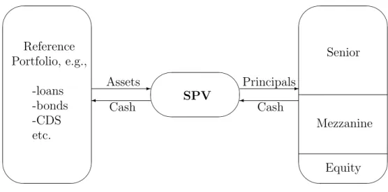
A CDO transaction has two sides – asset and liability – linked by cash flows (see Figure 1).
The asset side refers to the underlying reference portfolio while the liability side consists of securities issued by an issuer, which is often a special purpose vehicle (SPV). An SPV is a company created by an owner of a pool especially for the transaction, to insulate
'
&
$
%
Reference Portfolio, e.g.,
-loans -bonds -CDS etc.
'
&
$
%
SPV
'
&
$
%
Assets- Cash
Principals- Cash
Senior
Mezzanine
Equity
Figure 1: Illustration of a CDO cash flow mechanism.
investors from the credit risk of the CDO originator. An originating institution, usually a bank, sells assets to an SPV to manage exposure, shrink their balance sheets and reduce required capital but it often keeps the administration of the pool. The SPV claims the legal rights of the ownership of the credits and of all the cash flows arising from them.
To pay out to the originator for the collateral, SPV issues structured notes backed by the pool on its balance. The reference entities sold to the SPV are not at risk if either the SPV or the originator become insolvent. For that reason the SPV’s notes in the form of tranches receive better credit ratings and pay less interest than if they were issued by the bank.
CDOs are classified by types of underlying credits: collateralized loan/bond obligations are backed by loans/bonds, CDO-squared have collateral composed of other CDOs, see Bluhm et al. (2002). In this paper we apply the model to synthetic CDOs which are based on the pool of CDS because they are naturally structured as pure credit derivatives without involving any principal cash flows. Synthetic CDOs, in contrast to cash CDOs, transfer the risk away from the originator without the true sale of the collateral. Instead, the synthetic CDOs gain exposure to credit risk by selling protection through CDS contracts.
Synthetic CDOs can be either fully or partially funded. A fully funded CDO shifts the entire portfolio’s risk to the SPV via CDS. More typical are partially founded CDOs that transfer only the highest risk segment of the collateral.
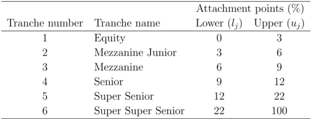
Each CDO tranche is defined by the detachment (lj) and attachment (uj) points which are the percentages of the portfolio losses. The first losses are covered by the equity tranche, also called a residual or a junior tranche. Table 1 presents the classic tranching taken from the iTraxx index. This example shows that the most subordinated tranche bears the first 3% losses of the portfolio nominal. The equity tranche holders are also paied an upfront fee. It is common that a bank keeps the riskiest piece. If losses constitute 5%
of the collateral notional, the equity investors carry the first 3% (thus loosing all their investment), and the next 2% is covered by those who invested in the mezzanine junior tranche. The tranches that carry the lowest risk are called senior tranches and get the highest credit ratings. They receive periodic income at first and as the last are affected
exceeds 22% of its notional value. Mezzanines have lower ratings than senior tranches but give better returns. The unrated equity tranche offers the highest coupons and gets paid at the end.
Attachment points (%) Tranche number Tranche name Lower (lj) Upper (uj)
1 Equity 0 3
2 Mezzanine Junior 3 6
3 Mezzanine 6 9
4 Senior 9 12
5 Super Senior 12 22
6 Super Super Senior 22 100
Table 1: Example of a CDO tranche structure, iTraxx.
Each loss that is covered reduces the notional on which the payments are based and also reduces the value of the periodic fee. After each default the seller of the protection makes a payment equal to the loss to the protection buyer. When the portfolio losses exceed the detachment point, no notional remains and no payment is made.
3 Univariate Credits: CDS
Synthetic CDOs, priced in this study, are backed by a portfolio of d CDS. A CDS is an insurance contract between two counterparties covering the risk that a specified credit defaults. The final result of the CDO calibration strongly depends on the evaluation of the risk of each underlying CDS contract. This section discusses the issues of calculating default probabilities and of the CDS valuation. For a survey of the CDS pricing please refer to Duffie (1999) and Hull & White (2000).
3.1 Default Probabilities
The individual default probabilities of the assets in the portfolio are a key input in the computation of the reference portfolio’s probability distribution. The modelling of the distribution consists of estimating the individual default probabilities and specifying the joint behaviour of the credits. The first step in pricing a multiname credit derivative is therefore to construct the default term structure of each underlying asset. Two models are in common use: structural and intensity. Structural models introduced by Hull &
White (2001) and further investigated by Hull, White & Predescu (2006) are based on the Merton (1974) approach in which a default occurs if the market value of the company’s assets falls below a value of fixed liabilities. Intensity models, also called reduced or hazard rate models, firstly introduced by Lando (1994) and Duffie & Singleton (1999), use prices
of defaultable securities traded on the market, like bonds, options or swaps. Default probabilities could also be computed from historical default rates provided by external rating agencies.
This study applies the intensity model to derive the default probabilities from the spreads of the CDS that underlie the iTraxx index. We assume the existence of a filtered proba- bility space (Ω,F,P) with a probability measure P. Let τ be a positive random variable representing the time of default of a given risky instrument, with a distribution function F. The term structure of default probability (the credit curve) is defined as:
p(t) = P(τ ≤t) =F(t) (1)
and represents the probability that an obligor defaults within the time interval [0, t]. In this framework the obligor’s default is modelled as the time until the first jump of a Poisson process with a deterministic or a stochastic intensity. The unconditional default probabilities are related to the intensity function λ(t) by the following equality:
p(t) = 1−exp
− Z t
0
λ(u)du
, (2)
where the corresponding survival probability term structure is given by:
¯
p(t) = 1−p(t) = P(τ > t). (3)
The probability that a default occurs in a small interval (t, t+∆t), given that the reference entity survived up to time t, is approximately
P(t < τ ≤t+ ∆t|Ft) = exp
−
Z t+∆t t
λ(u)du
Z t+∆t t
λ(u)du≈λ(t)∆t,
where{Ft :t >0}is the filtration that contains information about the underlying process till time t. Hence the intensity functionλ(t) has the following form:
λ(t) = lim
∆t→0
P(t < τ ≤t+ ∆t|Ft)
∆t (4)
and gives the instantaneous default probability of an asset that has attained aget. Mod- elling a default process is equivalent to modelling an intensity function. A homogeneous Poisson process corresponds to a constant intensity function λ(t) = λ, otherwise a pro- cess is called non-homogeneous. In practice, an intensity in form of a step function λ(t) = PTn
k=1αk1(Tk−1 < t ≤ Tk) is applied, where {Tk}nk=1 is a sequence of increas- ing maturities of the CDS contracts that have the same reference entity. The piecewise constant intensity incorporates more information and therefore gives a more realistic ap- proximation of the credit curve than a simple constant function. The parameters αk, k = 1, . . . ,n, are calibrated consecutively. First the intensity for the shortest maturityT1 is estimated. Havingα1 one estimates α2 from the CDS spread of the maturityT2 and so on. However, this approach requires significantly more market data input when dealing with large portfolios. In the case of the iTraxx collateral, it is difficult to provide spreads of several different maturities of 125 CDS contracts.
Credit default swaps were originally created as a means of shifting the default risk of a loan or a bond to a third-party. However, the CDS market changed so that sellers and buyers of contracts do not have to be owners of the underlying asset but are betting on the possibility of a credit event of a particular asset. Nowadays CDS are the most widely traded credit derivative products, mostly for speculative purposes.
Consider theith CDS from the CDO reference portfolio of d contracts, i= 1, . . . , d. We assume that the two parties of the transaction enter into the CDS on a trade date t0 and on this day the protection begins. For the iTraxx investor t0 express the time in years from the roll date of the iTraxx product untill the day for which the valuation is carried out. The protection buyer regularly pays premiums to a protection seller who in return agrees to cover losses if the ith company suffers a credit event. The value of the periodic fee is specified by the spreadsi(t0) of the CDS, the total notionalM and the time between the payment days. The protection buyer settles the cash obligations at predetermined dates, usually once per quarter, until the maturity T of the contract or until τi < T in the case of default. Thus on a payment day t the buyer of the CDS obtains an amount:
M si(t0)∆t1(τi > t),
where ∆t is a fraction of the year between t and the nearest preceding payment day and 1(·) is an indicator function. If the CDS defaults, the protection seller delivers a payoff equal to the notional value M of the obligation reduced by the recovery rate Ri:
M(1−Ri)1(τi ≤T)
and receives a part of the premium payment that has accrued since the last payment date:
M si(t0)(τi−t)1(t−∆t < τi ≤t).
The present value of the cumulated insurance payments made by the protection buyer during the life of the CDS is called a premium (fixed) leg P Li and equals
P Li(t0) =
T
X
t=t1
β(t0, t)M si(t0)∆tE{1(τi > t)}
=
T
X
t=t1
β(t0, t)M si(t0)∆texp
− Z t
t0
λi(u)du
,
wheret1 is the date of the first payment after the trade is made and the sum is taken over all scheduled payment days. All settlements are discounted to the time point t0 using the following discount factor:
β(t0, t) = (1 +rt/4)−4(t−t0)/365,
where rt is a compounded quarterly interest rate at time t. However, in the whole study rt is assumed to be constant.
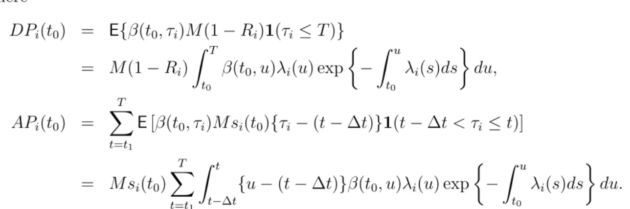
The present value of the payoff made by the protection seller in case of credit event is called default leg DLi and equals the expected present value of the contingent payment upon defaultDPi minus the contingent accrued premium APi:
DLi(t0) = DPi(t0)−APi(t0), where
DPi(t0) = E{β(t0, τi)M(1−Ri)1(τi ≤T)}
= M(1−Ri) Z T
t0
β(t0, u)λi(u) exp
− Z u
t0
λi(s)ds
du,
APi(t0) =
T
X
t=t1
E[β(t0, τi)M si(t0){τi−(t−∆t)}1(t−∆t < τi ≤t)]
= M si(t0)
T
X
t=t1
Z t t−∆t
{u−(t−∆t)}β(t0, u)λi(u) exp
− Z u
t0
λi(s)ds
du.
The values of both legs depend on the company’s tendency to default described by the intensity function λ(t). To emphasise that the premium’s value is driven by the intensity we write si(λi, t0). The CDS fair spread is then chosen in such a way that the market value of the contract is zero. On the trading day t0 the expected values of the sum of discounted payments made by the protection buyer and the protection seller must be equal P Li(t0) = DLi(t0), which implies
si(λi, t0) = E{β(t0, τi)(1−Ri)1(τi ≤T)}
PT
t=t1(β(t0, t)∆tE{1(τi > t)}+E[β(t0, τi){τi−(t−∆t)}1(t−∆t < τi ≤t)]). (5) Having the historical spreads of alldiTraxx underlying single-name CDS one can extract the default probabilities of these reference entities by inverting the pricing procedure and implying the intensity functions’ parameters. We calibrate the model to fit the CDS values, assuming that the intensity function is constant over time. The intensity that yields the quoted spread is found by applying a bisection method. We look for the solution of the equation si(ˆλi, t0) = si(t0), where si(t0) is the spread for the ith CDS quoted on the market. In Figure 2 we plotted the default probabilities calculated from the historical CDS spreads of Deutsche Bank with the maturity of 5 years.
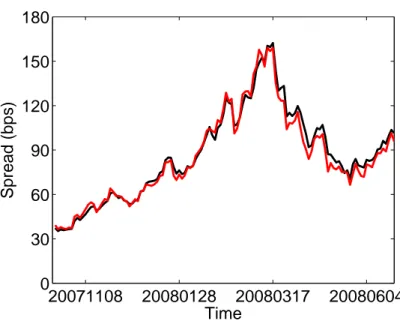
As the default probabilities are unobservable, the model used to estimate default prob- abilities can be verified by comparing theoretical iTraxx index spreads with real market quotes. The index spread ˜s at time t0 is not an arithmetic mean of CDS spreads but a survival probability weighted average:
˜ s(t0) =
Pd
i=1si(ˆλi, t0)PT
t=t1{1−pi(ˆλi, t)}/(1 +r/4)4t Pd
i=1
PT
t=t1{1−pi(ˆλi, t)}/(1 +r/4)4t , (6) where ˆλi is the intensity of theith company implied by the model, si(ˆλi, t0) is the spread defined in (5) with the probability of default denoted here by pi(ˆλi, t) and given by (2).
Figure 3 shows how the real market and the calibrated index spreads change over time. It can be seen that the estimation of the index is quiet precise which implies that the model reflects market behaviour well.
20071108 20080128 20080317 20080604 0
0.002 0.004 0.006 0.008 0.01 0.012
PD
Time
Figure 2: Probabilities of default (2) of Deutsche Bank, time period 20071022-20080630, R= 0.4,r = 0.03.
20071108 20080128 20080317 20080604 0
30 60 90 120 150 180
Spread (bps)
Time
Figure 3: Comparison of the market iTraxx index spreads (red) with the results of the model (6) (black), time period 20071022-20080630, R= 0.4, r= 0.03.
4 Multivariate Credits: CDO
The prices of the CDO tranches depend on the joint random behaviour of the assets in the underlying pool, more precisely, on their likelihood of joint defaults. The correlation is one of the most popular measures of dependence between two random variables. The standard market model for the CDO pricing, introduced by Li (2000), applies a multivari- ate Gaussian copula to describe the random co-movements of the reference entities. In addition, it assumes for simplicity, one value of the correlation for every pair of assets. An implied correlation can be calculated out of market spreads by inverting a pricing model.
The correlations implied from the different tranches of the same CDO are not equal and the observed phenomenon is called an “implied correlation smile”, see Bluhm & Overbeck (2006). There are several explanations for this inconsistency. One of the reasons might be an erroneous model. Thus it is of interest to investigate more flexible dependency structures which match the market spreads more accurately than the standard Gaussian one factor model.
4.1 Valuation of CDO
The CDO pricing is a two-step procedure. The main part of the valuation is the same for every approach and consists of defining the structure of payments that are made during the life of the contract. In the second, theoretical stage, the joint and marginal distributions of the reference entities need to be specified. The mechanism of cash flows between the protection seller and the protection buyer was presented in Section 2. We give below the necessary formulae that lead to a closed form of fair spreads of the CDO tranches. Similarly to the CDS, the fair spread is defined as a spread for which the market-to-market value of the contract is zero. This means that if the CDO originator pays the fair spread, the present value of the fee payments is equal to the present value of the contingent payments. Recall that theith obligor is deemed to default beforet ∈[t0, T] if τi ≤t. Then the loss variable is defined as:
Γi(t) =1(τi ≤t).
The portfolio loss process is the average of the all obligors’ losses:
L(t) = 1 d
d
X
i=1
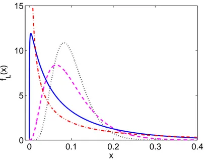
(1−Ri)Γi(t), t ∈[t0, T]. (7) Figure 4 represents the density function of the L(t) from the homogeneous one-factor Gaussian model for different values of the correlation parameter ρ. It shows that the correlation determines the shape of the portfolio distribution and hence the risk allocation between tranches.
The first losses are absorbed by the equity tranche until they reach a certain threshold.
The following losses are covered by more senior tranches. Consider a CDO of J tranches.
0 0.1 0.2 0.3 0.4 0
5 10
x f L(x)
Figure 4: Portfolio loss densityfL(·) for different correlation parametersρ: 0.05 (dotted), 0.1 (dashed), 0.3 (solid), 0.5 (dash-dot) and a fixed probability of default p= 10% in the HLPGC model.
The loss of the tranchej = 1, . . . , J, at time t is determined by its lower lj and upper uj
attachment point and the portfolio loss:
Lj(t) = min{max(0, L(t)−lj);uj−lj} (8)
=
0, L(t)< lj, L(t)−lj, lj ≤L(t)≤uj, uj−lj, L(t)> uj.
Similarly like in the case of the univariate contract, the present value of the sum of fee payments made by the protection buyer during the life of the CDO is called premium (fixed) leg. The protection seller receives insurance payments for which he obliges himself to cover losses affecting his tranche. The protection (floating, default) leg refers to the present value of the sum of contingent payments done upon credit events. The payments connected with tranche j at time t are calculated from the outstanding notional of the form:
Fj(t) = (uj−lj)−Lj(t), j = 1, . . . , J. (9) For the CDO valuation it is sufficient to determine the cumulative loss distribution at each payment day. This simplification allows avoiding a description of the whole path of the loss process but forces specification of the time of default between the payment days. The credit event can happen at any time but to get a close form solution we make a slightly simplifying assumption that all defaults occur in the middle of a payment period.
The premium leg P Lj is then based on the expected average of outstanding notionals from the two nearest payment days:
P Lj(t0) =
T
X
t=t1
β(t0, t)sj(t0)∆tE{Fj(t) +Fj(t−∆t)}M/2, j = 2, . . . , J. (10)
The premium leg can be expressed with the help of the risky duration RDj defined as:
RDj(t0) =
T
X
t=t1
β(t0, t)∆tE{Fj(t)}
uj−lj
, j = 2, . . . , J.
Then
P Lj(t0) = sj(t0)MRDj(t) +RDj(t−∆t)
2(uj −lj) , j = 2, . . . , J. (11) The most subordinated tranche is priced differently than the other tranches. The equity tranche pays an upfront fee once, at the inception of the trade and a fixed coupon of 500 bps during the life of the contract. The upfront payment, denoted by α, is expressed in percent and is quoted on the market. The premium leg of the residual tranche is defined as:
P L1(t0) =α(t0)(u1−l1)M +
T
X
t=t1
β(t0, t)·500·∆tE{F1(t) +F1(t−∆t)}M/2.
The protection leg DLj for all the tranches is calculated as follows:
DLj(t0) =
T
X
t=t1
β(t0, t)E{Lj(t)−Lj(t−∆t)}M, j= 1, . . . , J. (12) The premiumsj of the tranchej is chosen in such a way that both premium and protection legs are equal:
P Lj(t0) = DLj(t0).
This leads to the solution:
sj(t0) =
PT
t=t1β(t0, t)E{Lj(t)−Lj(t−∆t)}
PT
t=t1β(t0, t)∆tE{Fj(t) +Fj(t−∆t)}/2, for j = 2, . . . , J. (13) If we denote the denominator of the formula (13) by:
P L∗j(t0) =
T
X
t=t1
β(t0, t)∆tE{Fj(t) +Fj(t−∆t)}/2, (14) we get the fair spread of the form:
sj(t0) = DLj(t0)
P L∗j(t0) for j = 2, . . . , J. (15) For the equity tranche the upfront payment is equal to:
α(t0) = 100 u1−l1
T
X
t=t0
[β(t, t0)E{L1(t)−L1(t−∆t)} −500∆tE{F1(t) +F1(t−∆t)}/2]
= 100
u1−l1
{DLj(t0)/M −500P L∗j(t0)}.
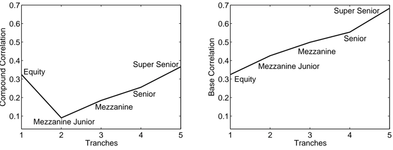
The CDO spreads sj(t0),j = 2, . . . , J, and the upfront feeα(t0) are constantly observed on the market. Our aim is to find a model that computes the prices which are close to the real values and which do not result in a formation of the implied correlation smile (see Figure 5, left panel).
1 2 3 4 5 0.1
0.2 0.3 0.4 0.5 0.6
Equity
Mezzanine Junior
Mezzanine Senior Super Senior
Tranches
Compound Correlation
1 2 3 4 5
0.1 0.2 0.3 0.4 0.5 0.6
Tranches
Base Correlation
Equity
Mezzanine Junior Mezzanine
Senior
Figure 5: Implied compound (left) and base (right) correlation smile from the HLPGC model. iTraxx Series 8 with maturity 5 years, from 20071022, R= 0.4, r= 0.03.
Types of Implied Correlation
There are two types of implied correlations: compound and base. The difference between them follows from distinct ideas of calculating the tranche losses (8). The survey of the implied correlations is provided by Finger (2004) and Willemann (2005). The implied compound correlation of a given tranchej is a parameter that makes the tranche spread computed by the model equal to its observed market value. The parameters implied from all tranches often form a smile shape which appears because the implied compound correlation for the equity and senior tranches turns out to be greater than that for the mezzanine tranches. For a correct model the implied correlation should be approximately constant for all tranches. Moreover, while implying the parameters, we come across non- existence and non-uniqueness of the implied compound correlation for mezzanine and more senior tranches. Sometimes two correlations reproduce the same tranche spread, in other cases we may not obtain any implied correlation at all.
These disadvantages are not possessed by the implied base correlations introduced by McGinty & Ahluwalia (2004). The numerical procedure of implying a base correlation uses a fact that the loss L(lj,uj) of a tranche (lj, uj) can be represented as a difference between losses of the two fictive equity tranches (0, uj) and (0, lj) defined as L(0,uj) and L(0,lj) respectively:
E{L(lj,uj)}=E{L(0,uj)} −E{L(0,lj)}, j = 2, . . . , J.
We fix a single correlation to price the (0, lj) tranche, then we look for a second correlation to price the (0, uj) tranche such that the spread difference is consistent with the observed (lj, uj) tranche spread. The base correlation are uniquely determined as the loss and the premium of the equity tranche always decreases with the correlation parameter. In addition, this measure allows to price the tranches that are not quoted on the market.
Since the base correlation depends only on a lower attachment point, we can use it to value off-market tranches by an interpolation approach. The comparison of the compound and the base correlation is shown in Figure 5.
4.2 Copulae
The use of copula functions allows for the specification of the default dependency of a high number of credits. We present below the necessary definitions and useful properties.
For a survey over the mathematical foundations of copulae we refer to Joe (1997) and Nelsen (2006).
A copula can be defined as an arbitrary distribution function on [0,1]d with all margins being uniform. The copula function captures the dependency between variables eliminat- ing the impact of the marginal distributions. Copulae gained a high degree of popularity due to the theorem of Sklar (1959). With Sklar’s theorem one can express the copula in the following way
C(u1, . . . , ud) = F{F1−1(u1), . . . , Fd−1(ud)}, u1, . . . , ud∈[0,1], where F1−1(·), . . . , Fd−1(·) are the corresponding quantile functions.
The elliptical cumulative distribution functions, like Gaussian and t-Student, generate the class of the elliptical copulae which have been, until now, of high interest in credit risk modelling. Another important group are Archimedean copulae. The d-dimensional Archimedean copula function C : [0,1]d→[0,1] is defined as
C(u1, . . . , ud) = φ{φ−1(u1) +· · ·+φ−1(ud)}, u1, . . . , ud ∈[0,1], (16) where φ ∈ {φ : [0;∞) → [0,1]|φ(0) = 1, φ(∞) = 0; (−1)jφ(j) ≥ 0;j = 1, . . . ,∞} is called a generator of the copula. In this study φ is assumed to be completely monotone.
Nevertheless, McNeil & Neˇslehov´a (2009) prove that the generator φ is required to be d- monotone, i.e. differentiable up to the orderd−2, with (−1)iφ(i)(x)≥0,i= 0, . . . , d−2 for any x∈[0,∞) and with (−1)d−2φ(d−2)(x) being nondecreasing and convex on [0,∞).
A prominent example is a Gumbel copula given by C(u1, . . . , ud;θ) = exp
−
( d X
j=1
(−loguj)θ )θ−1
with a generator
φ(x;θ) = exp{−x1/θ}, 1≤θ <∞, x∈[0,∞).
Note that (16) is symmetric with respect to the permutation of variables which entail that the distribution turns out to be exchangeable. Furthermore, for any dimension dthe multivariate structure depends on a single parameter of the generator functionφ.
Eachφ ∈ Lis a Laplace transform of some cumulative distribution function M of a posi- tive random variable, i.e. φ(t) = R∞
0 e−twdM(w). For an arbitrary cumulative distribution function F a unique cumulative distribution function G exists, such that
F(x) = Z ∞
0
Gα(x)dM(α) = φ{−logG(x)}.
F(x1, . . . , xd) = Z ∞
0
Gα1 · · · · ·GαddM(α)
= φ
(
−
d
X
i=1
logG(xi) )
=φ
" d X
i=1
φ−1{Fi(xi)}
# .
The above formula implies that the copula of F is given by (16). The representation of a copula in terms of a Laplace transform is very useful for simulating random numbers, see Whelan (2004), McNeil (2008), Marshall & Olkin (1988). The Laplace transforms allow for numerous interesting extensions. We can get a more general type of depen- dency by replacing the product copula Gα1· · ·Gαd with an arbitrary multivariate copula K(Gα1, . . . , Gαd) and by replacingM(α) with ad-variate distributionMd(α), such thatjth univariate margin has a Laplace transform φj, j = 1, . . . , d, see Joe (1997). Using these transformations we obtain a function called a fully nested copula of the form:
C(u1, . . . , ud) = Z ∞
0
. . . Z ∞
0
Z ∞ 0
Gα11(u1)Gα21(u2)dM1(α1, α2) (17)
×Gα32(u3)dM2(α2, α3). . . Gαdd−1(ud)dMd−1(αd−1).
Other orders of integration and combinations of the Gi functions lead to different forms of dependencies. In terms of the generators of the cumulative distribution functions M1, . . . , Md, the copula (17) can be rewritten as:
C(u1, . . . , ud) = φ1[φ−11 ◦φ2{. . .[φ−1d−2◦φd−1{φ−1d−1(u1) +φ−1d−1(u2)}+φ−1d−2(u3)] +. . . +φ−12 (ud−1)}+φ−11 (ud)]
= φ1{φ−11 ◦C2(u1, . . . , ud−1) +φ−11 (ud)}
= C1{C2(u1, . . . , ud−1), ud}.
The presented generalisation of the multivariate Archimedean copulae leads to the class of hierarchical Archimedean copulae (HAC). The profound study of HAC is provided by Okhrin et al. (2008) and Okhrin et al. (2009).
According to McNeil (2008), if φ1, . . . , φd−1 are completely monotonic generators and φi◦φi+1 have completely monotonic derivatives fori= 1, . . . ,d−1, then (17) is a proper copula function.
Note that generators φi within a HAC can come either from a single generator family or from different generator families. If φi belong to the same family, then the complete monotonicity of φi ◦φi+1 imposes some constraints on the parameters θ1, . . . , θd−1. For the majority of the copulae the parameters should decrease from the lowest to the highest level of a hierarchy to guarantee a feasible HAC. If φi are members of different families, then the complete monotonicity of φi◦φi+1 might not be fulfilled at all.
4.3 Joint Defaults
Assume that a CDO pool contains d CDS contracts whose individual risks are described with the credit curves pi(t) given by (2) or equivalently with the survival functions ¯pi(t)
given by (3), for i = 1, . . . , d and t ∈ [t0, T]. In the simulation study we consider that the ith obligor survives until t if and only if
Ui ≤p¯i(t), (18)
where a random variable Ui, called a trigger, is uniformly distributed on [0,1].
The difficulty in modelling the default risk of the CDO lies in finding the relation between default timesτ1, . . . ,τd of the underling securities. The main task consist of determining the joint distribution of the stopping times such that the marginal distributions are given by the credit curves. Multivariate copula functions provide a convenient way of specifing the joint distribution with given margins.
Note that the random variable ¯pi(τi) has the uniform distribution. Therefore the numbers U1, . . . , Ud have the same joint distribution as ¯p1(τ1), . . . , ¯pd(τd). The default times are obtained by taking the inverse of the survival functions in the points U1, . . . , Ud.
The joint distribution of the triggers satisfies:
C(u1, . . . , ud) = P(U1 ≤u1, . . . , Ud≤ud).
Applying the marginal survival probabilities at time t we obtain:
C{¯p1(t), . . . ,p¯d(t)}= P{U1 ≤p¯1(t), . . . , Ud ≤p¯d(t)}.
The above default time copula fully describes the non-linear dependency structure of its underlyings. The uniform marginal distributions of the copula ensure that theith margin is equal ¯pi:
P{Ui ≤p¯i(t)}= ¯pi(t).
The time to default variable
τi = inf{t≥t0 : ¯pi(t)≥Ui}, (19) is calculated as the first time when the process ¯pi(t) reaches the level of the trigger variable Ui. Assuming the constant intensities we simply compute that
τi = −logUi
λi .
The choice of the appropriate copula plays a crucial role in the final results. The selected function should represent desirable tail properties and the algorithm of generating the random numbers from it need to be known. The multi-parameter model can contain up to d(d−1)/2 parameters if the dependency is assumed to be Gaussian or t-Student and up to d−1 parameters for the HAC. In both situations the calibration of full models is unfeasible for larged and some techniques for reducing dimension have to be introduced.
The simplest way of handling the dimensionality in modelling the iTraxx data is to assume that all credits influence each other in the same way. Then a copula that define the relation between the portfolio’s components has only one parameter.
the iTraxx index, the CDS from the pool represent six industry sectors. To check whether we can identify the groups in data we applied a cluster analysis to the daily log-returns of the CDS spreads from 22 October 2007. The modified correlation matrix was used as a distance matrix. We obtained following six clusters: 9, 15, 17, 25, 28, 31. The result is similar to the true partition of the collateral what confirms that it is reasonable to include the sector aspect in the following research. Therefore we can construct the seven- parameter model in which the dependency in each group is described with a distinct one- parameter copula and the relations outside the groups are characterised with additional, seventh parameter. In such a case the correlation matrix has the following form:
R=
1 · · · ρ2
. ..
ρ2 · · · 1
ρ1 · · · · ...
ρ1
· · · ρ1 ... ... ρ1 · · · ρ1
... ...
1 · · · ρ3
. ..
ρ3 · · · 1
. ..
1 · · · ρ6
. ..
ρ6 · · · 1
... ... ρ1 · · · ρ1 ...
...
ρ1 · · · ·
ρ1
...
· · · ρ1
1 · · · ρ7
. ..
ρ7 · · · 1
(20)
When one deals with copulae, the correlation term ρ in the matrix above means, not Pearson linear correlation, but the Kendall’s or the Spearman’s rank correlation.
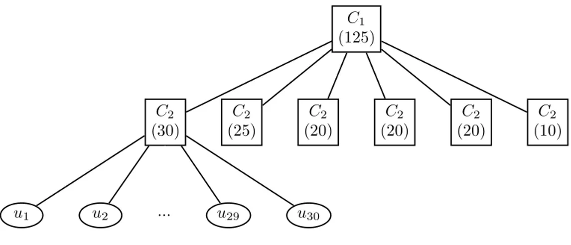
In the empirical study we will apply a simplification that assumes ρi =ρj and ρi 6=ρ1 for i, j = 2, . . . , 7. Then the model comprises the industry factor which imposes different inter- and intra-industry correlations. In the context of the Archimedean copluae the two-factor approach can be handled by HAC. Using the partially nested HAC we first describe the dependency within the industry sector with an Archimedean copulaC2 and then we join all groups with another Archimedean copula C1. The applied HAC has the following form:
C(u1, . . . , ud;θ) =C1{C2(u1, . . . , um1;θ2), C2(um1+1, . . . , um1+m2;θ2), . . . ,
C2(um1+...+m5+1, . . . , ud;θ2);θ1}, (21) where θ = (θ1, θ2)> and mk, k = 1, . . . , 6, indicates a number of the companies in kth industry sector. The graphical representation is shown in Figure 6. The Gaussian copula with sector correlations is discussed by Gregory & Laurent (2004).
When in (20) all parameters are equal, ρi = ρj for i, j = 1, . . . , 7, one deals with the one-factor model. If we, in addition, assume the normal copula, we get the standard
C1
(125)
C2
(30)
u1 u2 ... u29 u30
C2
(25) C2
(20) C2
(20) C2
(20) C2
(10)
Figure 6: Partially nested 125-dimensional HAC.
Gaussian copula model. Even though it is often criticized because of its simplifications, the Gaussian copula model still remains the benchmark on the market.
The appropriate multivariate distribution should reflect the tendency observed in financial data of joint extreme movements. That behaviour is described by the means of a tail dependence. The tail dependence gives the limiting proportion that some margins exceed a certain threshold conditional on the fact that others have already exceeded that threshold.
In the CDO framework the upper tail dependence allows us to quantify the risk that a CDS defaults (negation of (18) occurs) given that a different CDS defaults. The tail dependence is a property of a copula function and is independent of marginal distributions.
The normal distribution is asymptotically tail independent so by its construction is unable to handle the extremal dependence. For that reasons we will focus on a Gumbel copula which exhibits the upper tail dependence. The Gumbel copula is suitable to describe the outcomes that are likely to simultaneously realize upper tail values. The different tail behaviour of the Gauss and Gumbel copula is clearly visible in Figure 7 showing the contour plots of the 3-dimensional one and two-parameter copula densities.
The tail dependence of a bivariate distribution is deeply studied by Joe (1997). A com- mon measure of the bivariate tail dependence is given by the so-called tail dependence coefficient. Several generalisations to the multivariate tail dependence have been pro- posed. Schmidt & Stadtm¨uller (2006) present tail copulae that describe the dependence structure of multi-dimensional distributions in the tail. The tail dependence functions are also discussed by Kl¨uppelberg, Kuhn & Peng (2008) and Nikoloulopoulos, Joe & Li (2008).
4.4 Loss Given Default
Because of the high complexity of the CDO valuation it is a common practice to introduce simplifications and to neglect some of the parameters. Most of the models that are used to reproduce the tranche spreads assume the constant recovery rate and one value of the default probability equal for all the underlying credits, see f.e. Hofert & Scherer (2008).
Kendall’s rank correlation 0.6. Isosurface of the Gauss (bottom left) and Gumbel (bottom right) copula density with Kendall’s rank correlations 0.5 and 0.8. Margins are modelled with the standard normal distribution.
However, as the spreads are calculated not on the total amount of the losses but only on its fraction that cannot be recovered, the loss given default has the significant effect on the final value of the payments. In the following proposition we take advantage of the finding of Altman, Brady, Resti & Sironi (2005) and Hamilton, Varma, Ou & Cantor (2005) who show that the recovery rate is stochastic and strongly negatively correlated with the default probabilities.
There is no standard method of modelling the recovery rate. Nevertheless many ways of introducing the recovery rate to the default risk modelling have been proposed. The stochastic recovery rate is also applied by Jarrow (2001) and Andersen & Sidenius (2005).
Duffie & Singleton (1999) assume the recovery to be a proportion of the market data value, which is random but the recovery proportion is fixed. Hull & White (2004), Hull
& White (2006) use the recovery rate that is fixed over time and for all obligors. Duffie
& Gˆarleanu (2001) take it as a uniform random variable and Hull et al. (2006) assume that in the Gaussian copula framework it follows a beta distribution. However, Scaillet &
Renault (2004) estimate the recovery rate density nonparametrically using a beta kernel method and parametrically using a beta distribution calibrated on the empirical mean
C1
(126)
C2
(125)
u1 u2 ... u124 u125
LGD
Figure 8: HAC with the random loss given default.
and variance. The nonparametric density estimates shows that the recovery rate is not beta distributed. Sch¨onbucher (2003) models the recovery of a defaulted obligor with a logistic normal process. R¨osch & Scheule (2005) propose a multifactor-model for defaults and recoveries. Das & Hanouna (2009) find that the identification of the recovery rate and default intensities is infeasible using only the term structure of CDS spreads. They provide a jump-to-default model that uses the stock prices and the stock volatility with credit spreads to identify the implied functions of the recovery rate and the default probability.
Pan & Singleton (2008) handle with the identification problem and propose a model which separately identifies the parameters through the information contained in the term structure of CDS contract.
In the following section we propose a method of modelling the relation between the joint default times and the loss given default. We keep the assumption of the constant recovery rate in the univariate model for CDS contracts, but we bring in the additional random- ness to the CDO valuation. The high dimensionality of the collateral forces us to apply the same loss given default for all the underlyings. However, we apply copula functions that enable us to reflect the observed relations. We have already pointed out that the Gumbel copula is characterised by interesting properties which make it suitable for credit risk modelling. In the next step we will focus on this family while developing the model.
As the Gumbel copula can only represent positive dependence, we introduce the depen- dence between the default times and the loss given default. For our problem we apply hierarchical Archimedean copulae composed of Gumbel copulae of different dimensions.
As there is no clear evidence on the specific distribution of the loss given default we leave it uniformly distributed on [0,1].
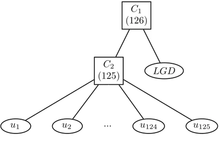
The first proposition is the straightforward extension of the one-parameter model. The hierarchical structure integrates the loss given default with the default times as illustrated in Figure 8. The applied copula has the following form:
C(u1, . . . , ud, ud+1;θ) = C1{ud+1, C2(u1, . . . , ud;θ2);θ1}, (22) where θ = (θ1, θ2)>. On the first level the whole pool of credits is modelled with a 125-dimensional copula C2 with the parameter θ2 as was done in the simplest case. The
(126)
C2
(125)
C3
(30)
u1 u2 ... u29 u30
C3
(25) ... C3
(20) C3
(10) LGD
Figure 9: HAC with the random loss given default and the sector structure.
second level joins the defaults and the loss given default with a 126-dimensional copula C1 with the parameterθ1. A similar approach has been recently investigated by H¨ocht &
Zagst (2009).
Another model incorporates the natural structure of the CDO pool and is visualised in Figure 9. The corresponding copula function is given by:
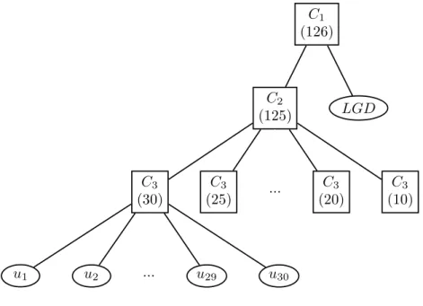
C(u1, . . . , ud, ud+1;θ) =C1[ud+1, C2{C3(u1, . . . , um1;θ3), C3(um1+1, . . . , um1+m2;θ3), . . . , C3(um1+...+m5+1, . . . , ud;θ3);θ2};θ1], (23) whereθ = (θ1, θ2, θ3)>. The lowest level of the hierarchy connects the defaults within the sectors of the CDO collateral. The middle stage joins the six sectors. The highest level aggregates the loss given default and the Archimedean copula from the previous level.
The possible extension of this approach could be to introduce distinct loss given defaults for each sector. Then the copula would have the following form:
C(u1, . . . , ud, . . . , ud+6;θ) = C1[C2{ud+1, C3(u1, . . . , um1;θ3);θ2},
C2{ud+2, C3(um1+1, . . . , um1+m2;θ3);θ2}, . . . ,
C2{ud+6, C3(um1+...+m5+1, . . . , ud;θ3);θ2};θ1], (24) where θ = (θ1, θ2, θ3)>. We start by coupling random variables within sectors. At the second level we connect each sector with the loss given default. The final stage consist of joining the subgroups with the 131-dimensional copula. (23) and (24) require the estima- tion of three parameters, however the complexity of last method makes it computationally expensive and involves time demanding simulations.