CDO Surfaces Dynamics

SFB 649 Discussion Paper 2013-032

CDO Surfaces Dynamics

Barbara Choroś-Tomczyk*

Wolfgang Karl Härdle*

Ostap Okhrin*

* Humboldt-Universität zu Berlin, Germany

This research was supported by the Deutsche

Forschungsgemeinschaft through the SFB 649 "Economic Risk".

http://sfb649.wiwi.hu-berlin.de ISSN 1860-5664

SFB 649, Humboldt-Universität zu Berlin Spandauer Straße 1, D-10178 Berlin

SFB

6 4 9

E C O N O M I C

R I S K

B E R L I N

CDO Surfaces Dynamics ^∗

Barbara Choro´s-Tomczyk

, Wolfgang Karl H¨ ardle

, Ostap Okhrin

July 2, 2013

Abstract

Modelling the dynamics of credit derivatives is a challenging task in finance and economics. The recent crisis has shown that the standard market models fail to measure and forecast financial risks and their characteristics. This work studies risk of collateralized debt obligations (CDOs) by investigating the evolution of tranche spread surfaces and base correlation surfaces using a dynamic semiparametric factor model (DSFM). The DSFM offers a combination of flexible functional data analysis and dimension reduction methods, where the change in time is linear but the shape is nonparametric. The study provides an empirical analysis based on iTraxx Europe tranches and proposes an application to curve trading strategies. The DSFM allows us to describe the dynamics of all the tranches for all available maturities and series simultaneously which yields better understanding of the risk associated with trading CDOs and other structured products.

Keywords: base correlation, collateralized debt obligation, curve trade, dynamic factor model, semiparametric model.

JEL classification: C14, C51, G11, G17

1 Introduction

The recent financial crisis began in 2007 with the subprime mortgage crisis in U.S. Then it spread globally and gathered intensity in 2008. The financial system weakened and remained frozen. In 2009 the global economy stabilized but has not returned to its pre- crisis levels.

Collateralized debt obligations (CDOs) played a significant role in the global financial crisis. A CDO is a credit derivative used by financial institutions to repackage individ- ual assets into a product that can be sold to investors on the secondary market. The

∗The financial support from the German Research Foundation, Project HA2229/7-2 and via CRC 649 Economic Risk at Humboldt-Universit¨at zu Berlin is gratefully acknowledged.

†Ladislaus von Bortkiewicz Chair of Statistics, C.A.S.E. – Center for Applied Statistics and Economics, Humboldt-Universit¨at zu Berlin, Unter den Linden 6, 10099 Berlin, Germany.

‡Corresponding author. Email: barbara.choros@wiwi.hu-berlin.de

§School of Business, Singapore Management University, 50 Stamford Road, Singapore 178899

assets may be mortgages, auto loans, credit card debt, corporate debt or credit default swaps (CDS). CDOs were initially constructed for securitization of big portfolios. The entire portfolio risk is sliced into tranches and then transfered to investors. Prior to the credit crisis, CDOs provided outstanding investment opportunities to market participants.

Banks used CDOs to reduce the amount of debt on their balance sheets. Tranching made it possible to create new securities of different risk classes that met the needs of a wide range of clients. The market observed an excess demand for senior CDO tranches because they were considered as safe and offered unusual high returns. As we know now, the rat- ing agencies underestimated default risk of CDOs. Consequently, investors were exposed to more risk than the ratings of these CDOs implied. When the market collapsed, CDO investors faced enormous losses that led some of them to bankruptcy (Lehman Brothers) or a takeover (Bear Stearns, Merrill Lynch) by another institutions. The CDO market has significantly shrunk the beginning of the financial crisis. However, the methodology proposed in our study can be used in modelling and trading other financial instruments, especially non-standardised and bespoke structured products.

Developments in the CDO research mainly concern finding an accurate and flexible pricing model, see a comparison of popular models in Bluhm & Overbeck (2006) and Burtshell, Gregory & Laurent (2009). Papers that investigate implied correlations concentrate on the replication of the shape of the implied curve, e.g. A˘gca, Agrawal & Islam (2008).

Primarily because of the high dimensionality of the CDO problem the vast majority of papers consider only CDOs of one particular maturity, see e.g. Hamerle, Igl & Plank (2012). Up to our knowledge, the available literature do not look at the CDO market as a whole. Since CDOs are quoted for different maturities, we should consider the effect of the CDO term structure.

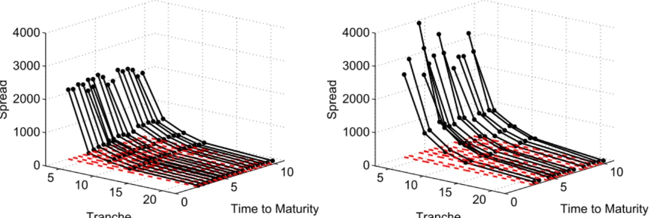
The empirical research of this study was performed using the iTraxx indices and their tranches of Series 2 to 10. The iTraxx Europe is the most widely traded credit index in Europe. Its reference portfolio consists of 125 equally weighted, most liquid credit default swaps (CDS) on European companies. Twice a year, every March and September, a new series of iTraxx is issued and the current constituents are reconsidered. The iTraxx Europe trades at maturities of 3, 5, 7 and 10 years. The tranches with 5 years maturity are the most liquid, unlike those with 3 years maturity that are rarely quoted. Because of the regular index roll, each day one observes on the market tranches with various times to expiration. By plotting prices of all available tranches at one day as a function of the time to maturity and the tranche seniority, one gets a surface that represents entire market information about spreads, see Figure 1. Similarly, an implied base correlation surface can be constructed. When we record these surfaces every day, we can follow how they change their shape and level. The dynamics over time of such surfaces is the main goal of this paper. From an investor’s point of view, it is desirable to have an insight into the behaviour of spreads and base correlations in the future. The forecasting has useful applications in hedging and trading CDOs, like computation of Greeks, risk measures, or construction of investment strategies. One of the simplest solutions would be to consider the classic time series analysis for each tranche of each series for every maturity. Due to illiquidity and due to the short history of particular series, this methodology is not applicable. Thus, the natural choice for CDO data is to first interpolate observations

5 10 15 20 0 5 10 0

1000 2000 3000 4000

Time to Maturity Tranche

Spread

5 10 15 20 0 5 10

0 1000 2000 3000 4000

Time to Maturity Tranche

Spread

Figure 1: Spreads of all tranches of all series observed on 20080909 (left) and 20090119 (right).

for each time point by creating a smooth surface and afterwards to forecast this new high-dimensional object.

High-dimensional data sets naturally appear in many fields of science ranging from fi- nance to genetics. Worth mentioning statistical approaches for handling complex high- dimensional problems are a structural analysis of curves by Kneip & Gasser (1992), a stochastic warping model by Liu & M¨uller (2004), penalized splines by Kauermann, Krivobokova & Fahrmeir (2009), and a functional principal components approach by Gromenko, Kokoszka, Zhu, & Sojka (2012). One of the most popular methods are factor type models as they effectively reduce the dimensionality. Factor models assume that the comovements of big number of variables are generated by a a small set of latent fac- tors. When data disclose a dynamic structure then one needs a technique that is able to correctly detect and describe the observed behaviour, e.g. Gourieroux & Jasiak (2001), Hallin & Liˇska (2007), Koopman, Lucas & Schwaab (2012). In this study we employ a dynamic semiparametric factor model (DSFM).

In the DSFM the observed variables are expressed as linear combinations of the factors.

The factors and the factor loadings are estimated from the data. The first ones represent the spatial, time-invariant component. The later ones form multidimensional time series that reflect the dynamics. The inference on the original variables reduces to the inference on the factors and the factor loadings.

The DSFM was introduced by Fengler, H¨ardle & Mammen (2007) for modelling the dynamics of implied volatility surfaces. Further, Giacomini, H¨ardle & Kr¨atschmer (2009) apply the DSFM to analyse risk neutral densities implied by prices of DAX options, H¨ardle, Hautsch & Mihoci (2012) use it for limit order book analysis, Detlefsen & H¨ardle (2013) for variance swaps, and Myˇsiˇckov´a, Song, Majer, Mohr, Heekeren & H¨ardle (2013) for fMRI images. In this work we study the dynamics of CDO surfaces with the DSFM and propose an application to curve trading strategies.

The paper is structured as follows. Section 2 discusses the CDO valuation. Section 3 describes the DSFM. Section 4 shows results of the empirical modelling. Section 5 presents applications in CDO trading. Section 6 concludes.

2 Collateralized Debt Obligations

Consider a CDO with a maturity of T years, J tranches and a pool of d entities at the valuation dayt₀. A tranchej = 1,. . . , J absorbs losses betweenl_j percent andu_j percent of the total portfolio loss. l_j and u_j are called an attachment and a detachment point respectively and l_j < u_j. For the iTraxx Europe, successive tranches have the following attachment points: 0%, 3%, 6%, 9%, 12%, 22%. The corresponding detachment points are 3%, 6%, 9%, 12%, 22%, 100%.

The protection buyer pays periodically to the protection seller a predetermined premium, called a spread on the outstanding tranche notional and is compensated for losses that occur within the range of the tranche. Each default in the portfolio reduces the notional on which the payments are based. This leads to a decline in the value of the periodic fee.

The cash exchange takes place until the maturity of the CDO or until the portfolio losses exceed the detachment point.

This section briefly discusses key points of the CDO pricing. First, we describe the cash- flow structure. Then we specify the distribution of the portfolio losses. At the end we present a concept of a base correlation.

2.1 Valuation

We assume that there exists a risk-neutral measure P under which the discounted asset prices are martingales. The expectations in the formulas below are taken with respect to this measure.

The loss of the portfolio of d assets at timet is defined as L(t) = LGD

d

d

X

i=1

Γ_i(t), t∈[t₀, T], (1)

where LGD is a common loss given default and Γi(t) =1(τi ≤t),i= 1,. . . ,d, is a default indicator showing that the credit i defaults at timet within the period [t₀, T] if the time of default random variableτ_i ≤t. The loss of a tranchej = 1, . . . , J at timet is expressed as

L_j(t) = L^u(t, u_j)−L^u(t, l_j),

with L^u(t, x) = min{L(t), x}, x ∈ [0,1]. The outstanding notional of the tranche j is given by

F_j(t) = F^u(t, u_j)−F^u(t, l_j),

with F^u(t, x) = x−L^u(t, x), x ∈ [0,1]. At the predefined dates t = t₁, . . . , T, t₁ > t₀, the protection seller and the protection buyer exchange the payments. The protection leg DL_j is defined as the present value of all expected payments made upon defaults

DL_j(t₀) =

T

X

t=t1

β(t₀, t)E{L_j(t)−L_j(t−∆t)}, j = 1, . . . , J, (2)

where β is a discount factor and ∆t is a time between t and the previous payment day.

The premium leg PLj is expressed as the present value of all expected premium payments PL_j(t₀) =

T

X

t=t1

β(t₀, t)s_j(t₀)∆tE{F_j(t)}, j = 2, . . . , J, (3) where s_j denotes the spread of tranche j. The first tranche, called the equity is traded with an upfront payment α and a fixed spread of 500 bp. Its premium leg (3) turns into

PL₁(t₀) = α(t₀)(u₁−l₁) +

T

X

t=t1

β(t₀, t)·500·∆tE{F₁(t)}.

A spreads_j is calculated once, at t₀ so that the marked-to-market value of the tranche is zero, i.e. the value of the premium leg equals the value of the protection leg

sj(t0) = PT

t=t1β(t₀, t)E{L_j(t)−L_j(t−∆t)}

PT

t=t1β(t0, t)∆tE{Fj(t)} , for j = 2, . . . , J. (4) The upfront payment of the equity tranche is computed as

α(t0) = 100 u₁−l₁

T

X

t=t0

(β(t, t0) [E{L1(t)−L1(t−∆t)} −0.05∆tE{F1(t)}]).

For more details we refer to Bluhm & Overbeck (2006) and Kakodkar, Galiani, J´onsson

& Gallo (2006).

The iTraxx data used in this study cover years 2005–2009 when the tranches were priced in the way presented above. However, since 2009 the quoting convention of the iTraxx Europe tranches has changed. Now all the tranches (0-3%, 3-6%, 6-9%, 9-12%, 12-22%, 22-100%) have a structure of the equity tranche and trade with an upfront fee and a fixed running spread of 500 bp, 500 bp, 300 bp, 100 bp, 100 bp, and 25 bp respectively.

2.2 Credit risk models

The main challenge in calculating the fair tranche spread (4) is the correct calculation of the expected losses. This task requires the analysis of how the portfolio entities are likely to default together. At the core of the CDO pricing lies a dependency model for portfolio credit risk. There are two main types of credit risk models: structural and reduced form models. The structural model is motivated from a Merton style approach where a default occurs when the value of an asset drops below a certain level. In the reduced form approach a default is modeled with an intensity process. A third class is based on copula theory and is connected with the first two approaches. For a comprehensive overview we refer to Bielecki & Rutkowski (2004).

There has been a multitude of CDO risk models proposed that apply different dependency concepts. The market standard for pricing CDOs is the large pool Gaussian copula model

that has been introduced to the valuation of multi-name credit derivatives by Li (2000).

The large pool concept is also the basis of the Gaussian one-factor model proposed by Vasicek (1987).

In the Vasicek model, an obligor i = 1, . . . , d defaults before time T if the value of a random variable Xi drops below a thresholdCi

P(τ_i ≤T) = P(X_i < C_i).

The variableX_i is defined as a linear combination of the systematic risk factorY and the idiosyncratic risk factor Z_i

X_i =√

ρY+p

1−ρZ_i, (5)

In this setting Y and {Z_i}^d_i=1 are i.i.d. N(0,1) variables. Thus, {X_i}^d_i=1 follow a multi- variate Gaussian distribution with an equal pairwise correlation ρ.

The model assumes that the portfolio is large and homogeneous, i.e. it possesses an infinite number of assets that have the same exposure, default probability, loss given default, correlation and that these values are constant over all time horizons. The individual default probability determines the default threshold C_i =C = Φ⁻¹(p) for all i = 1, . . . , d, where Φ denotes the cdf of the standard normal distribution.

The portfolio loss distribution is approximated by the conditional probability given the common factor Y. When Y is fixed, the conditional default probability of any obligor is given by

p(y) =P(X_i < C|Y =y) = Φ

C−√

√ ρy 1−ρ

. (6)

Conditional on the realization of the common factor, the variables (5) are independent.

The portfolio loss conditional on Y converges, by the law of large numbers, to its expec- tation p(y). The cdf of the loss of a very large portfolio is in the limit equal

P(L≤x) =P{p(Y)≤x}= Φ √

1−ρΦ⁻¹(x)−Φ⁻¹(p)

√ρ

. (7)

The expected tranche loss in (2) and (3) is calculated as an integral with respect to the distribution (7) and because of absence of the explicit solution it has to be evaluated numerically.

The main drawback of the Gaussian copula is that it exhibits no tail dependence and in consequence it cannot model the extreme events accurately. However, due to its ana- lytical tractability and numerical simplicity, the Gaussian copula model still remains the benchmark on the market.

2.3 Base correlation

In the Gaussian copula model the main driver of the tranche price is the correlation coefficient. The correlations can be computed from market data by inverting the pricing

formula (4). If we keep the value of other parameters fixed, then the correlation parameter that matches the quoted tranche spread is called an implied compound correlation. It is observed that implied compound correlations are not constant across the tranches. This phenomenon is called an implied correlation smile. Still, the main disadvantage of the compound coefficient is that the mezzanine tranches are not monotonic in correlation and two parameters might result in the same spread value. The second problem that we might encounter is a nonexistence of the implied correlation. These disadvantages caused the enhanced popularity of base correlations proposed by McGinty & Ahluwalia (2004).

The main idea behind the concept of the base correlation is that each tranche [l_j, u_j] can be represented as a difference of two, equity type tranches that have the lower attachment point zero: [0, uj] and [0, lj]. Here we use a property that the equity tranche is monotone in correlation. The base correlations can be implied from the market spreads using standard bootstrapping techniques. One needs the spread value of the tranche [uj−1, u_j] and the base correlation of the tranche [0, uj−1] in order to imply the base correlation [0, u_j]. In this approach, (4) is calculated as

s_j(t₀) = PT

t=t1β(t₀, t)

E_ρ(0,uj){L^u_j(t, u_j)−L^u_j(t−∆t, u_j)}−E_ρ(0,lj){L^u_j(t, l_j)−L^u_j(t−∆t, l_j)}

PT

t=t1β(t₀, t)∆t

E_ρ(0,uj){F_j^u(t, u_j)} −E_ρ(0,lj){F_j^u(t, l_j)}

(8) for j = 2, . . . , J, where the expected value E_ρ(0,uj) is calculated with respect to the dis- tribution (7) determined by the base correlation ρ(0, uj) of the tranche [0, uj]. In the Gaussian copula model the base correlations are nondecreasing with respect to the se- niority of tranches and the implied correlation smile turns into a correlation skew.

3 Dynamic Semiparametric Factor Model

Let Yt,k be a data point, a tranche spread or a base correlation, observed on a day t, t= 1, . . . , T. The indexk represents an intra-day numbering of observations on that day, k = 1, . . . , K_t. The observationsY_t,k are regressed on two-dimensional covariatesX_t,kthat contain the tranche seniority and the remaining time to maturity

Y_t,k =m₀(X_t,k) +

L

X

l=1

Z_t,lm_l(X_t,k) +ε_t,k, (9) where m_l :R² → R, l = 0, . . . , L, are factor loading functions, Z_t,l ∈ R are factors, and ε_t,j are error terms with zero means and finite variances.

The additive structure of (9) is a typical approach in regression models. Here, the func- tions m are estimated nonparametricly and represent the time-invariant, spatial compo- nent. The factorsZ_tdrive the dynamics ofY_t. The number of factorsLis fixed and should be small relative to the number of observed data points so that we achieve a significant reduction in the dimension. The investigation of the dynamics of the entire system boils down to the analysis of the factors’ variability. These arguments justify calling (9) a dynamic semiparametric factor model.

Fengler et al. (2007) estimatemandZ_titeratively using kernel smoothing methods, Song, H¨ardle & Ritov (2013) apply functional principal component analysis, Park, Mammen, H¨ardle & Borak (2009) estimate m with a series based estimator. For numerical con- venience we follow the last paper and define functions ψ_b : R² → R, b = 1, . . . , B, B ≥ 1, such that R

R²ψ_b²dx = 1. Then, a tuple of functions (m₀, . . . , m_L)^> may be ap- proximated by Aψ, where A is a (L+ 1×K) matrix of coefficients {{a_l,b}^L+1_l=1 }^B_b=1 and ψ = (ψ₁, . . . , ψ_B)^>. We take {ψ_b}^B_b=1 to be a tensor B-spline basis. For a survey over the mathematical foundations of splines we refer to de Boor (2001). With this parametrization (9) turns into

Y_t,k =Z_t^>m(X_t,k) +ε_t,k =Z_t^>Aψ(X_t,k) +ε_t,k, where Z_t= (Z_t,0, . . . , Z_t,L)^> with Z_t,0 = 1 and m= (m₀, . . . , m_L)^>. The estimates Zbt = (Zbt,0, . . . ,Zbt,L)^> and Abare obtained by

(Zb_t,A) = arg minb

Zt,A T

X

t=1 Kt

X

k=1

Y_t,k−Z_t^>Aψ(X_t,k) ², (10) yielding estimated basis functions mb = Aψ. The minimization is carried out using anb iterative algorithm. However, the estimates ofm andZt are not uniquely defined. There- fore, the final estimates ofm are orthonormalized and Z_tare centered. Park et al. (2009) also prove that the difference of the inference based on the estimated Zb_t,l and the true, unobserved Z_t,l is asymptotically negligible. This result justifies fitting an econometric model, like a vector autoregressive to the estimated factors for further analysis of the data.

The number of factors L as well as the numbers of spline knots in both maturity and tranche directions R₁, R₂, and the orders of splines r₁, r₂ have to be chosen in advance.

A common approach is to maximize a proportion of the variation explained by the model among the total variation. We propose a following criterion

EV(L, R₁, r₁, R₂, r₂) = 1− PT

t=1

PKt

k=1

n

Y_t,k−PL

l=1Z_t,lm_l(X_t,k)o2

PT t=1

PKt

k=1{Y_t,k−me₀(X_t,k)}² , (11) where

me₀(X_`) = 1 T

T

X

t=1

PKt

k=1Y_t,k1{X_` =X_t,k} PKt

k=11{X<sub>`</sub> =X<sub>t,k</sub>} , ` = 1, . . . , K_max, (12) is an empirical mean surface and K_max is the number of all different X_t,k observed during T days. The criterion (11) is a modified version of this considered in Fengler et al. (2007) and other literature on the DSFM, where instead of the empirical mean surface, the overall mean of the observations is used. The mean surface (12) makes more sense, since our data reflect monotonous behaviour w.r.t. the time to maturity.

The me₀ factor in (9) is usually interpreted as a mean function of the data. We propose to first subtract the estimate (12) from the data and then fit the DSFM. The extraction of the empirical mean me₀ leads to the following model

Y_t,k =me₀(X_t,k) +

L

X

l=1

Z_t,lm_l(X_t,k) +ε_t,k=me₀(X_t,k) +Z_t^>Aψ(X_t,k) +ε_t,k, (13)

where m_l are factor functions, l = 1, . . . , L, Z_t,l are factor loadings, and A is a (L×B) coefficient matrix. The representation (13) reduces the number of the factor functions estimated in the iterative algorithm (10). The model (9) is the classic DSFM and we will refer to it as the DSFM. The model (13) is hereafter called the DSFM without the mean factor.

4 Modelling the Dynamics of CDO Surfaces

4.1 Data Description

The data set analysed in this study contains daily spreads of iTraxx tranches of Series 2 to 10 between 30 March 2005 (hereafter denoted 20050330) and 2 February 2009 (denoted 20090202) obtained from Bloomberg. We have in totalPT

t=1K_t= 49502 data points over T = 1004 days. As far as we know, this is the first study on CDOs that consider such an extensive data set.

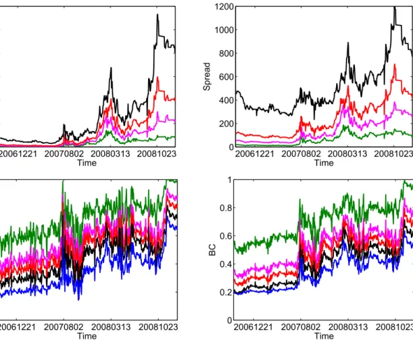
Each index has 3, 5, 7, or 10 years maturity. Figure 2 shows the market spreads of Series 6 and the corresponding implied Gaussian base correlations for the maturity of 5 and 10 years. We see similarities in the general evolution between these two maturities. However, since their exposure in terms of duration differs, they represent different levels.

Due to the issuing scheme one observes every day a bunch of indices from various series and different maturities. Here we analyse tranche spreads and also base correlations, both denotedY_t, as a function of the tranche seniorityξ_tand the remaining time to maturityτ_t. The seniority of a tranche ξ_t is represented by its corresponding detachment point. The remaining time to maturity of an index is an actual time left till its expiration and takes values between zero and 10.25. For every day a separate surface representing the market information is available. The number of observed every day indices is low (minimum 4, maximum 17, median 12, see Figure 3). This results in a string structure in the data.

Each string corresponds to one τ_t ∈[0,10.25] and is composed out of at most five points.

The market quotes five out of six tranches as the most senior tranche is usually not traded.

Figure 1 and Figure 4 present the curves of market spreads and corresponding implied base correlations on 20080909 and 20090119. As time passes, the curves move through the space towards expiry and simultaneously change their skewness and level. As previously mentioned, the main aim of this research is to model the evolution of the iTraxx spreads and base correlations simultaneously in space and time dimensions.

Since the shortest maturity is 3 years and every half a year new four indices are issued, the number of indices present on the market grows in time. Table 1 shows the number of observed market values of iTraxx tranches for every possible maturity during the entire period considered and during the annual subperiods. Table 2 outlines a percentage of missing values for every maturity and for every tranche. We see that the CDO market was booming in 2006 and 2007. However, since the beginning of the financial crisis in 2008 the demand for credit derivatives had been shrinking meaningfully. In the first quarter of

20061221 20070802 20080313 20081023 0

200 400 600 800 1000 1200

Spread

Time 020061221 20070802 20080313 20081023

200 400 600 800 1000 1200

Spread

Time

20061221 20070802 20080313 20081023 0

0.2 0.4 0.6 0.8 1

BC

Time 020061221 20070802 20080313 20081023

0.2 0.4 0.6 0.8 1

BC

Time

Figure 2: Market spreads (upper panel) and implied base correlations (lower panel).

Series 6, maturity 5 (left) and 10 (right) years. Data from 20060920-20090202. Tranches:

1 (blue), 2 (black), 3 (red), 4 (pink), 5 (green).

20050831 20060905 20070910 20080912 0

5 10 15 20

Time

Figure 3: Daily number of curves for every surface during the period 20050330-20090202.

10 5

20 15 0

5 10 0

0.5 1

Time to Maturity Tranche

BC

10 5

20 15 0

5 10 0

0.5 1

Time to Maturity Tranche

BC

Figure 4: Base correlations of all series observed on 20080909 (left) and 20090119 (right).

2009 the iTraxx tranches became highly illiquid. Many missing data may create challenges to the econometric analysis. Because tranches with 3 years maturity were rarely traded, this maturity was excluded from our study. Tables 3 and 4 present summary statistics of

Year 3Y 5Y 7Y 10Y

2005 0 1478 715 1532

2006 181 3998 3739 4005 2007 75 5155 5170 5172 2008 232 5904 5916 5932

2009 0 260 263 263

All 488 16740 15803 16840

Table 1: Number of observed values of iTraxx tranches in the period 20050330-20090202.

Year 3Y 5Y 7Y 10Y

1 2 3 4 5 1 2 3 4 5 1 2 3 4 5 1 2 3 4 5

2005 100 100 100 100 100 34 34 34 34 48 5 5 5 5 5 35 34 35 34 35

2006 78 56 55 100 100 6 7 6 6 8 3 3 3 4 4 5 5 6 8 6

2007 88 99 99 100 100 3 2 2 3 3 2 2 3 2 3 3 2 3 2 2

2008 47 99 100 100 100 24 25 25 24 27 24 25 25 25 27 24 27 24 25 24 2009 100 100 100 100 100 42 42 47 42 42 42 43 43 42 42 42 43 42 42 43 All 72 93 93 100 100 16 17 17 16 20 13 14 13 13 14 16 17 16 17 16

Table 2: Percentage of missing values during the period 20050330-20090202.

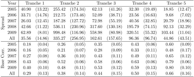
Year Tranche 1 Tranche 2 Tranche 3 Tranche 4 Tranche 5

Spread

2005 40.90 (13.22) 255.42 (174.34) 62.13 (41.26) 32.30 (19.49) 18.85 (12.47) 2006 33.71 (14.76) 212.75 (173.46) 52.09 (38.71) 23.56 (16.63) 9.68 (7.02) 2007 26.03 (12.45) 187.28 (127.72) 72.98 (55.19) 40.56 (32.85) 20.79 (18.96) 2008 42.66 (11.22) 536.11 (230.96) 317.60 (130.18) 195.79 (74.15) 92.13 (32.29) 2009 62.89 (8.01) 998.48 (116.96) 558.98 (80.98) 320.51 (55.32) 103.44 (11.04) All 35.56 (14.86) 335.27 (256.95) 162.61 (157.65) 96.36 (96.74) 44.86 (43.51)

BaseCorr.

2005 0.18 (0.04) 0.26 (0.05) 0.35 (0.05) 0.43 (0.06) 0.60 (0.09) 2006 0.16 (0.05) 0.21 (0.07) 0.28 (0.09) 0.33 (0.11) 0.48 (0.17) 2007 0.27 (0.08) 0.36 (0.10) 0.43 (0.11) 0.49 (0.11) 0.65 (0.12) 2008 0.43 (0.06) 0.52 (0.06) 0.58 (0.06) 0.63 (0.06) 0.79 (0.06) 2009 0.40 (0.10) 0.48 (0.11) 0.53 (0.12) 0.59 (0.13) 0.80 (0.10) All 0.29 (0.13) 0.38 (0.14) 0.44 (0.15) 0.50 (0.15) 0.66 (0.16)

Table 3: Mean and standard deviation (in parentheses) of tranche spreads (UFF for the tranche 1) and implied base correlations during the period 20050330-20090202.

Year Index

2005 46.34 (11.08) 2006 37.70 (11.86) 2007 40.22 (16.25) 2008 121.71 (50.86) 2009 205.47 (44.04) All 77.25 (57.60)

Table 4: Mean and standard deviation (in parentheses) of iTraxx indices’ spreads during the period 20050330-20090202.

the market spreads, the base correlations, and of the iTraxx indices.

Sometimes on a particular day, for a particular tranche and a particular remaining time to maturity we observe two different spreads. As an example consider a dayt₀ on which a new series with 3 years maturity is issued. If 5 years earlier a series with 7 years maturity was issued, then on day t0 this series has also 3 years remaining time to maturity. In this situation we include in our data set the observation that comes form the most actual series (in the example we take the series issued on t₀).

The base correlations (8) are implied from the market spreads using the large pool Gaus- sian copula model (assuming the LGD of 60%) presented in Section 2.2. The common intensity parameters are derived from iTraxx indices. The discount factors are calculated from rates of Euribor and Euro Swaps.

The structure of the equity tranche is different from the other tranches. It is quoted as an upfront payment plus 500 bp spread paid quarterly. In order to include the equity tranche in the joint analysis of all the tranches, we convert its quotes to standard spreads with zero upfront fee using the large pool Gaussian copula model.

4.2 DSFM Estimation Results

Since our data are positive and monotone, we convert spreads into log-spreads and for base correlations apply the Fisher’s Z-transformation defined as

T(u) = arctanh(u) = 1

2log 1 +u 1−u.

It transforms the empirical Pearson’s correlations between bivariate normal variables to a normally distributed variable. We will use it for the base correlations as it stabilizes their variance.

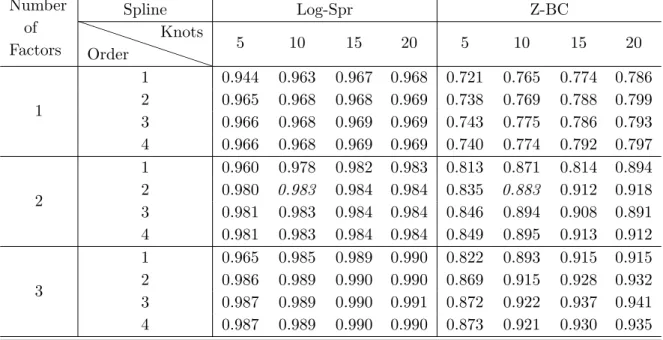
As discussed in Section 3, the number of factors L, the numbers of knots R₁, R₂, and the orders of splines r1, r2 are selected according to (11). Since the design of the data in the tranche seniority dimension is fixed, we choose in this direction quadratic B-splines and five knots. Tables 5 and 6 present a proportion of the explained variation (11) by the DSFM and the DSFM without the mean factor respectively for different numbers of factors, knots and different orders of splines in the maturity dimension. Similar like in Park et al. (2009), we find that the order of splines and the number of knots have a small influence on the proportion of the explained variation. We pick the quadratic B-splines placed on 10 knots in τ dimension for both types of data and for both DSFM models.

The number of knots is close to the median number of observed strings every day. Table 7 outlines the criterion’s values for the chosen tensor B-splines and for up to five factors.

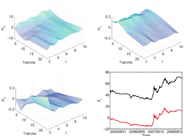
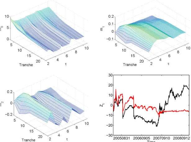
The information shown there reveals that two factors are sufficiently good approximation to the data. Figures 5 and 6 exhibit mb and Zb_t in the DSFM for the log-spreads and the Z-transformed base correlations respectively. Figures 7 and 8 show the DSFM without the mean factor estimates.

Number of Factors

Spline Log-Spr Z-BC

PP PP

PP PP

P Order

Knots

5 10 15 20 5 10 15 20

1

1 0.944 0.963 0.967 0.968 0.721 0.765 0.774 0.786 2 0.965 0.968 0.968 0.969 0.738 0.769 0.788 0.799 3 0.966 0.968 0.969 0.969 0.743 0.775 0.786 0.793 4 0.966 0.968 0.969 0.969 0.740 0.774 0.792 0.797

2

1 0.960 0.978 0.982 0.983 0.813 0.871 0.814 0.894 2 0.980 0.983 0.984 0.984 0.835 0.883 0.912 0.918 3 0.981 0.983 0.984 0.984 0.846 0.894 0.908 0.891 4 0.981 0.983 0.984 0.984 0.849 0.895 0.913 0.912

3

1 0.965 0.985 0.989 0.990 0.822 0.893 0.915 0.915 2 0.986 0.989 0.990 0.990 0.869 0.915 0.928 0.932 3 0.987 0.989 0.990 0.991 0.872 0.922 0.937 0.941 4 0.987 0.989 0.990 0.990 0.873 0.921 0.930 0.935 Table 5: Proportion of the explained variation by the DSFM for L = 1, 2, 3, different numbers of knots and different orders of splines in the maturity dimension. The values of the selected models marked with italic.

Number of Factors

Spline Log-Spr Z-BC

PP PP

PP PP

P Order

Knots

5 10 15 20 5 10 15 20

1

1 0.797 0.876 0.897 0.898 0.629 0.640 0.660 0.660 2 0.877 0.896 0.905 0.910 0.633 0.654 0.657 0.664 3 0.867 0.898 0.906 0.908 0.638 0.650 0.662 0.664 4 0.871 0.898 0.907 0.910 0.639 0.653 0.659 0.662

2

1 0.842 0.925 0.940 0.945 0.730 0.835 0.860 0.869 2 0.926 0.952 0.961 0.954 0.781 0.861 0.876 0.888 3 0.911 0.952 0.941 0.950 0.763 0.867 0.883 0.887 4 0.917 0.956 0.947 0.954 0.783 0.870 0.881 0.886

3

1 0.858 0.940 0.959 0.973 0.746 0.854 0.888 0.898 2 0.941 0.967 0.977 0.982 0.815 0.896 0.907 0.925 3 0.927 0.967 0.975 0.979 0.805 0.901 0.922 0.930 4 0.932 0.972 0.977 0.982 0.817 0.903 0.910 0.927 Table 6: Proportion of the explained variation by the DSFM without the mean factor for L= 1, 2, 3, different numbers of knots and different orders of splines in the maturity dimension. The values of the selected models marked with italic.

Number of Factors

DSFM DSFM w/o mean f.

Log-Spr Z-BC Log-Spr Z-BC

1 0.968 0.769 0.896 0.654

2 0.983 0.893 0.952 0.862

3 0.989 0.919 0.967 0.887

4 0.991 0.931 0.973 0.909

5 0.993 0.936 0.976 0.918

Table 7: Proportion of the explained variation by the models withL= 1, . . . , 5 dynamic factors and quadratic tensor B-splines placed on 5×10 knots.

20050831 20060905 20070910 20080912

−20 0 20 40 60 80

Z t

Time

Figure 5: Estimated factors and loadings (Z_t,1 black, Z_t,2 red) in the DSFM for the log-spreads.

20050831 20060905 20070910 20080912

−20

−10 0 10 20 30

Z t

Time

Figure 6: Estimated factors and loadings (Zt,1 black, Zt,2 red) in the DSFM for the Z-transformed base correlations.

20050831 20060905 20070910 20080912

−30

−20

−10 0 10 20 30

Z t

Time

Figure 7: Sample mean, estimated factors and loadings (Z_t,1 black,Z_t,2 red) in the DSFM without the mean factor for the log-spreads.

20050831 20060905 20070910 20080912

−10 0 10 20 30 40

Z t

Time

Figure 8: Sample mean, estimated factors and loadings (Zt,1 black,Zt,2 red) in the DSFM without the mean factor for the Z-transformed base correlations.

In the DSFM for both data types, the first and the second factor can be interpreted as a slope-curvature and a shift function respectively. Increasing Zbt,1 results in the enhance- ment of the surface’s steepness, whereas, decreasing Zb_t,1 implies its flattening. When we shiftZb_t,2, the whole surface shifts along thez-axis. In the DSFM without the mean factor for the log-spreads we observe an opposite influence of the factors. Namely,mb₁ is the shift factor, mb₂ is the slope-curvature factor. For the DSFM without the mean factor applied to the Z-transformed base correlations the interpretation is not so clear. When varying Zbt,1 and Zbt,2 both the slope and the curvature change. The upward shift of the surface can be a result of a decrease in Zb_t,1 or an increase in Zb_t,2.

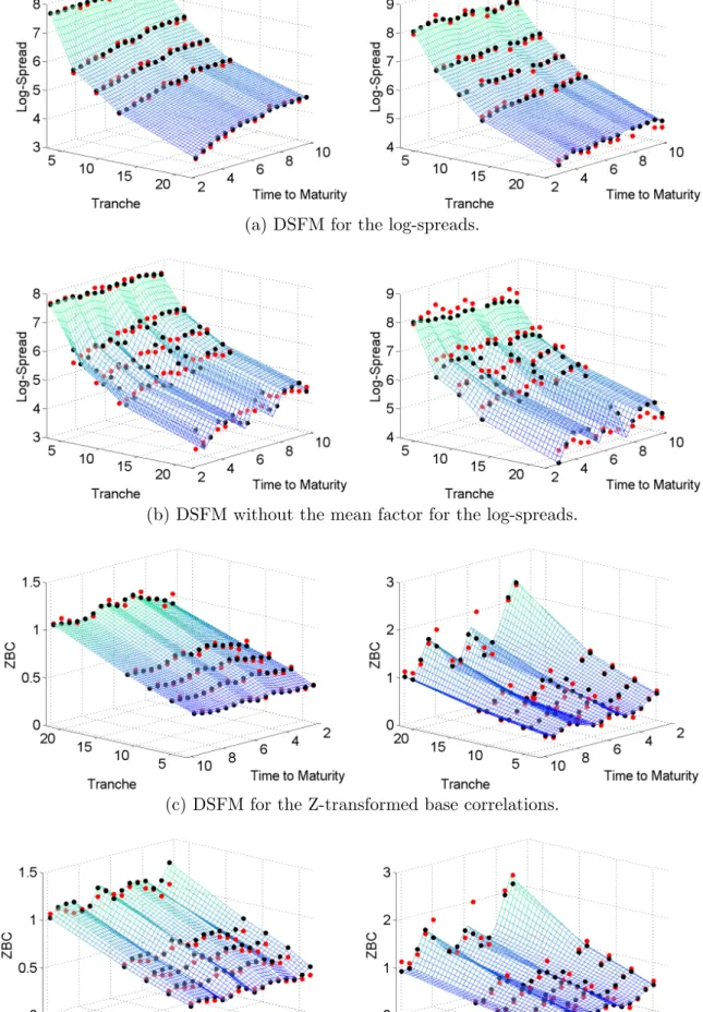
Table 8 discloses the mean squared error of the in-sample fits. The classic DSFM occurs to provide a better fit to the data than the DSFM without the mean factor. Moreover, the Z-transformed base correlations are approximated more accurately than the log-spreads for both DSFMs. Figure 9 displays the in-sample fit of the models to data on 20080909 and 20090119. The convergence of the models is typically reached after 8 cycles.

Model Log-Spr Z-BC

DSFM 0.016 0.004

DSFM w/o mean f. 0.045 0.006 Table 8: Mean squared error of the in-sample fit.

The covariance structure of the Zb_t time series is investigated by means of VAR analysis.

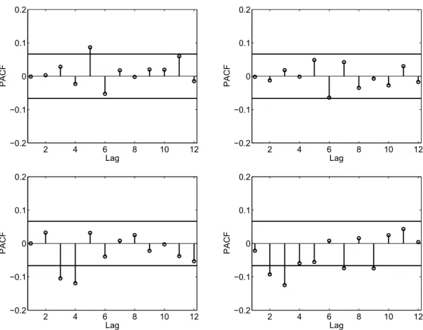
The augmented Dickey-Fuller test indicates that the first differences ofZb_t in both DSFMs are stationary. Figure 10 exhibits the sample partial autocorrelation functions of the residuals of the estimated VAR(1) models for the factor loadings of the DSFM without the mean factor. In general only a few autocorrelations lie slightly outside the 95% confidence interval. A similar result is observed for the classic DSFM. Thus, VAR(1) seems to be in line with the data. Certainly, one may investigate more complex multivariate time series models that account for a dynamic structure of the conditional variance-covariance and of the conditional correlation like the BEKK-GARCH or the DCC-GARCH, see Engle (2002). Since we are interested in the conditional mean process only, the VAR model appears to be sufficient. Moreover, a relatively simple out-of-sample VAR forecasting can be used in forecasting the evolution of the surfaces.

5 Applications in Trading

5.1 Curve Trades

The popularity of the iTraxx market led to more liquidity in its standardized tranches allowing investors to implement complex credit positions. Here we present curve trades, namely flatteners and steepeners – strategies that combine tranches of different time to maturity, see also Kakodkar et al. (2006).

(a) DSFM for the log-spreads.

(b) DSFM without the mean factor for the log-spreads.

(c) DSFM for the Z-transformed base correlations.

(d) DSFM without the mean factor for the Z-transformed base correlations.

Figure 9: In-sample fit (black points) of the models to data (red points) on 20080909 (left) and 20090119 (right).

2 4 6 8 10 12

−0.2

−0.1 0 0.1 0.2

Lag

PACF

2 4 6 8 10 12

−0.2

−0.1 0 0.1 0.2

Lag

PACF

2 4 6 8 10 12

−0.2

−0.1 0 0.1 0.2

Lag

PACF

2 4 6 8 10 12

−0.2

−0.1 0 0.1 0.2

Lag

PACF

Figure 10: Sample partial autocorrelation for VAR(1) residuals of the factor loadings Z_t,1 (left) and Z_t,2 (right) in the DSFM without the mean factor for log-spreads (upper panel) and Z-transformed base correlations (lower panel). The solid lines correspond to the approximate lower and upper 95% confidence bounds.

A flattener is a trade that involves a simultaneous sale of a long-term tranche and a purchase of a short-term tranche. An example would be: sell 10Y 3-6% and buy 5Y 6-9%. In this trade the investor expresses a bullish long-term outlook but also a bearish short-term view on the market. The opposite trade is called a steepener. It is achieved by selling the short-term protection and buying the long-term protection. Both strategies are popular in trading CDS, credit indices, and yield curves. Credit curves got a lot of attention in May 2012 when J.P. Morgan announced a loss of $2 billion on its flattener trade on the CDX IG 9 index. The final loss reached $6.2 billion.

In our study both long and short term tranches have equal notional amounts. However, by adjusting the notionals, a trade can be structured so that it is risky duration neutral, carry neutral, correlation neutral, or theta (sensitivity to implied correlation changes) neutral, see Roy (2007). As recommended by Felsenheimer, Gisdakis & Zaiser (2004) we consider trades that generate no or a positive carry, i.e. the spread of the sold protection does not exceed the spread of the bought protection.

It is important to remark that very often our trades will be exposed to jump-to-default risk. For simplicity, let us consider in this paragraph flatteners only. If one buys 5Y 6-9%

and sells 10Y 6-9%, then the trade is fully hedged for default only until the maturity of the 5Y tranche, i.e. any defaults that emerage from 10Y 6-9% are covered by 5Y 6-9%

till it expires. It should also be pointed out that the tranches do not have to be from the same series and there are slight differences in the composition of the collaterals of every series. Another case is if one buys 5Y 6-9% and sells 10Y 3-6%, then these tranches provide protection of different portion of portfolio risk. If there is any default in 10Y 3-6%, then we must deliver a payment obligation and incur a loss. Since we do not posses data of historical defaults in iTraxx, we cannot include the default payments in the further analysis. Consequently, in calculating the profit-and-loss (P&L) of the strategy we also do not account for the positive carry that we cumulate until the both positions are closed.

Felsenheimer et al. (2004), Kakodkar et al. (2006) and Roy (2007) consider various sce- narios of flattener trades. They also assume that we do not observe any defaults in the collateral. However, the examples are not based on real data and do not investigate the performance of the trades over time.

Assume that an investor enters a curve trade and sells protection at a spread of s1(t0) for the period [t₀, T₁] and buys protection at a spread of s₂(t₀) for the period [t₀, T₂]. If the trade is a flattener, thenT₁ > T₂. The spreads of the tranches are calculated in such a way that on the date of the trade t₀ the marked-to-market (MTM) values of both positions are zero

MTM_`(t₀) =

T`

X

t=t1

β(t₀, t) [s_{`</sub>(t<sub>0</sub>)∆tE{F<sub>`}(t)} −E{L_{`</sub>(t)−L<sub>`}(t−∆t)}] = 0, `= 1,2.

Since spread values constantly vary over time, immediately after initiation of the trade,

˜t > t0, the market trades the tranches at s`(˜t). In consequence, we observe a change in the MTM value of our positions

MTM_`(˜t) =

s_{`</sub>(t<sub>0</sub>)−s<sub>`}(˜t)

T_`

X

t=˜t1

β(˜t, t)∆tE{F<sub>`</sub>(t)}, `= 1,2, (14)

where ˜t₁ is the first payment day after ˜t.

A positive MTM means that the contract has a positive value to the protection seller.

If the protection seller closes the position ` at time ˜t, then receives from the protection buyer the amount MTM<sub>`</sub>(˜t).

The aim of the curve trade investor is to maximize the P&L function that equals the total MTM value

PL(˜t) = MTM₁(˜t)−MTM₂(˜t). (15)

5.2 Empirical Results

The key decision in constructing a curve trade is which tranche to buy and which to sell.

If an investor entered a flattener on 20080909, then the trade incorporated two tranches whose spreads are depicted on the left panel of Figure 1. If the investor decided to close

the positions on 20090119, then their MTM values (14) were calculated using the spread quotes exhibited on the right panel of Figure 1 and using the base correlations (need for E{F_`}) shown on the right panel of Figure 4. Having the data displayed on Figures 1 and 4, we can compute the MTM values of all tranches that where quoted on both days. In consequence, we can easily recover those two tranches that maximize the P&L function (15). However, it is only possible if we possess the whole market information from these two points in time.

With an efficient forecasting technique, one can compute a prediction, for a given time horizon, of each point that is displayed on the left panels of Figures 1 and 4. By doing it using standard econometric methods, each tranche from every series has to be treaded as an individual time series. Disregarding the fact that there are many missing values in our data, see Table 2, we have many series that do not have a long history. If an investor bought a tranche from Series 9 on 20080320, the day of its launch and decided to sell it a day or a week later, then we might not have enough past observations to fit and forecast the model.

In the DSFM modelling we do not differentiate the indices by their series number but by their remaining time to maturity. If in the past we already had observations with a very long remaining time to maturity, then we are able to price upcoming series even before they appear on the market. Moreover, we can forecast them using the DSFM.

We carry out the forecasting of log-spreads and Z-transformed base correlations in mov- ing windows. A moving window procedure is used when only the most recent data are considered to be relevant for the estimation. We impose a static window ofw= 250 days.

Then for every time t₀ between the day w and the last day T in our data, we analyse {Y_t}^t_t=t⁰ _0−w+1. For these sequences the DSFMs (9) and (13) are estimated separately. As a result, we obtain T −w+ 1 times the estimated factor functions mb = (mb₀, . . . ,mb_L)^>

and the series of the factor loadings Zb_t = (Zb_t,0, . . . ,Zb_t,L)^> of length w. Since the factor functions are fixed, the forecasting is performed only on the factor loadings. As discussed in Section 4.2, we apply VAR(1) models to compute the predictions for a horizonhof one day, one week (five days), and one month (20 days). Due to the fixed scheme of issuing the iTraxx on the market, for every time t, w+h≤t≤T we know which indices are traded.

Therefore, the number of points that could be observed K_t and the possible remaining times to maturity τ_t are known. Thus, the bivariate vector X_t,k, k = 1, . . . , K_t, does not have to be forecasted. The forecastYbt is calculated from theZbtforecast. Finally, a proper inverse transformation is applied to Yb_t in order to recover the values of the spreads and the base correlations.

The calculation of the expected tranche losses needs as an input a homogeneous default probability, see (7). Since the spread predictions are calculated out-of-sample, we also forecast the default probabilities. The time series of the default probabilities are derived from the time series of all the iTraxx indices considered and are forecasted with an AR(1)- GARCH(1,1) process in moving windows of w observations. For short data histories we reduce the window size or take as a predictor the last observed value. All predicted values of spreads and base correlations that lead to an arbitrage in prices, i.e. negative spreads, default probabilities and base correlations outside [0,1], were excluded.

Afterwards, for every predicted{ˆs_k(t),ρˆ_k(t)},t =w+h, . . . , T,k = 1, . . . , K_t, we compute MTM\k(t) according to (14) where the initial spread is the spread observed on t −h.

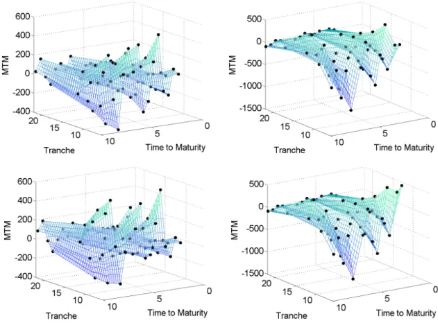
Consequently, we create a surface of the predicted MTM values, see Figure 11. Each surface has its extremes that indicate the tranches recommended for buying and selling.

Figure 11: MTM surfaces on 20080909 (left) and 20090119 (right) calculated using one-day spread and base correlation predictions obtained with DSFM (upper panel) and DSFM without the mean factor (lower panel).

The empirical analysis of the curve trades’ performance is conducted using tranches 2-5 for all dates and indices considered in Section 4.2. Since the equity tranche is quoted in percent as an upfront fee, its corresponding spread is significantly higher than the spreads of other tranches. As it causes a large skew of our spread surfaces, we excluded it from the study. In addition, we also avoid the multiple conversion of the upfront fee to the spread and back.

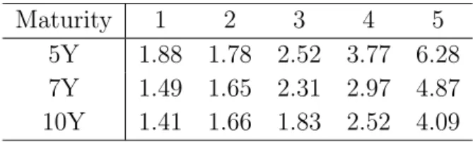
Buying and selling tranches involve transaction charges. However, we do not have in- formation on trading costs neither the entire history of the bid and ask prices. We only analyse the bid-ask spreads of Series 8. Table 9 shows an average distance of the bid spread and of the ask spread from the mid spread as a percentage of the mid spread.

For the investigation of the trading strategies, the tranche spread data used in this study are adjusted in the following way. The protection buyer delivers an ask spread that is calculated as a mid spread increased by a proper percent listed in Table 9. The protection seller receives a bid spread which is calculated as a mid spread reduced by this percentage.

The calculation of the spread and the MTM value of the tranche 2 requires as an input a

Maturity 1 2 3 4 5 5Y 1.88 1.78 2.52 3.77 6.28 7Y 1.49 1.65 2.31 2.97 4.87 10Y 1.41 1.66 1.83 2.52 4.09

Table 9: Average bid-ask spread excess over the mid spread as a percentage of the mid spread for Series 8 during the period 20070920-20090202

value of the base correlation of the equity tranche. Therefore, we conduct a preliminary analysis of the models (9) and (13) using all tranches and in this way obtain the forecast of the first tranche’s parameter.

For every dayw≤t≤T −hwe construct a curve trade. Namely, we fit and forecast the DSFM models and calculate h-day forecasts of the MTM surfaces. From these surfaces we recover which two tranches and from which series optimize a given strategy. We can e.g. consider a flattener that from all existing indices always buys the maturity 7Y, sells 5Y, and selects only the tranche 2. For a flattener and a steepener one can restrict the choice to a fixed tranche and fixed maturities or choose from all tranches and from all maturities. We also include a strategy that allows the investor to switch between flatteners and steepeners every day. If a strategy that combines flatteners and steepeners allows in addition choosing any tranche and any maturities, then the selected tranches are the maximum and the minimum of the forecasted MTM surface. If we consider the flatteners only, then we have to comply with the constraintτ₁−τ₂ >0. If for a particular day there are no tranches that for a given strategy return a positive P&L forecast, we assume that the investor decides not to take any action and we do not include this date in the overall summary of this strategy.

The accuracy of the predictions is evaluated by conducting a backtesting of the trades using the historical observations. For a given strategy and for the tranches selected by the DSFM forecasting procedures we check the corresponding observed market spreads, calculate the resulting MTM values, and register the realised P&L. Table 10 presents the overall means of the daily gains of different strategies given in percent. The labels in the first column should be read in the following way. Each name is composed of three parts joined with a hyphen. The first part indicates the type of the curve trade: flattener (F), steepener (S). The first five rows present results of the trades that combine flatteners and steepeners (FS). The second element of the name shows which tranches were considered:

all tranches (AllT), only tranche 2 (T2), etc. The last part expresses the maturities taken:

all maturities (AllM), 5Y and 10Y (510), etc. In the case of considering all maturities it is possible that the optimal strategy is composed of two tranches that have the same maturity, e.g. both are 5Y, but they come from different series and in consequence their remaining time to maturity are different. The spread predictions can alternatively be computed directly from the base correlations predictions by using (8). As a consequence it is not necessary to apply DSFMs to historical spreads. Table 10 presents also the results obtained by modelling and forecasting the Z-transformed base correlations only. Table 11 discloses the number of executed trades during the whole time period. Table 12 exhibits the corresponding Sharpe ratios calculated as the mean over the standard deviation.

To summarize the trading algorithm we enumerate its steps:

1. Consider a static rolling window of w and a forecasting horizon h.

2. For every t=w, . . . , T −h estimate the DSFMs (9) and (13) using{Y_ν}^t_ν=t−w+1. 3. Compute the forecast Zb_t+h using a VAR model.

4. Check what the possible X_t+h are and calculateYb_t+h. 5. Transform Yb_t+h suitably to get ˆs(t+h) or ˆρ(t+h).

6. Compute the surface of forecasted MTM values with (14).

7. Select two tranches according to the strategy’s restrictions.

8. Calculate the predicted P&L with (15).

9. Check the historical spread values for the selected tranches on day t+h. Imply the base correlations, calculate the realised MTM values and the realised P&L.

The results show that the highest daily gains where achieved by the strategies that invest in tranche 2 and 3. Obviously these tranches are quoted at the highest spreads but also carry the greatest risk. The steepeners for a fixed tranche and fixed maturities reveal a very good performance. However, as compared with Table 11 these strategies were rarely carried out which means that the conditions of these strategies were difficult to meet.

The performance of the DSFM model (9) and (13) is comparable. The models based entirely on the predictions of the base correlations achieve better results for one-day and one-week forecasting horizon. The models that combine the spread predictions and the base correlations predictions show better results for one-month forecasting horizon. Since the forecasting for the longer time horizons is less accurate, we observe a significantly better performance of the trades designed for short term periods.

The curve trades can be also tested from the perspective of an investor that follows a certain strategy over long time horizon and constantly rebalances the trade. Assume that at t₀ the investor enters an optimal curve trade for h-day horizon. At t₀ +h she either keeps the current position for the nexth-days or closes it and enters a new one. In addition, we assume a margin of 10% of the notional. Every time the position is closed its gain is added or its loss is subtracted from the margin. If the loss exceeds the margin, the trade is closed. Otherwise, the investor follows her strategy for one year (250 days).

If at ˜tthere are no positions that give a positive P&L forecast, the investor waits till ˜t+ 1 and repeats the check.

We analyse a strategy of combined flatteners and steepeners from all tranches and all maturities using our entire data set. Figure 12 displays the final cumulated gains after one year of the investor as a function of the date on which the investor planed to finish trading (i.e. the starting date plus one year). The seasonality pattern observed on the plots appears because the strategy with h-day rebalancing constructed on day t₀ and on day t₀+h might overlap. If on t₀ we started a 250-days strategy with a trade that was closed after h-days then a strategy started on t₀+h differ from the previous one by the first and the last step only. Figure 13 shows an over time performance of the investor’s trades started on 20070614 and closed on 20080529. The final cumulated profits equal 39.08%, 35.87%, and 20.35% when the account is rebalanced each day, week, and month respectively. These values are the last points depicted on the right plots on Figure 13 and they are presented on Figure 12 for the day 20080529.