Veröffentlichungen der DGK
Ausschuss Geodäsie der Bayerischen Akademie der Wissenschaften
Reihe C Dissertationen Heft Nr. 825
Niclas Zeller
Direct Plenoptic Odometry –
Robust Tracking and Mapping with a Light Field Camera
München 2018
Verlag der Bayerischen Akademie der Wissenschaften
ISSN 0065-5325 ISBN 978-3-7696-5237-6
Diese Arbeit ist gleichzeitig als E-Dissertation auf mediaTUM veröffentlicht:
https://mediatum.ub.tum.de/?id=1402349
Veröffentlichungen der DGK
Ausschuss Geodäsie der Bayerischen Akademie der Wissenschaften
Reihe C Dissertationen Heft Nr. 825
Direct Plenoptic Odometry –
Robust Tracking and Mapping with a Light Field Camera
Von der Ingenieurfakultät Bau Geo Umwelt der Technischen Universität München
zur Erlangung des Grades Doktor-Ingenieur (Dr.-Ing.) genehmigte Dissertation
Vorgelegt von
M. Eng. Niclas Zeller
Geboren am 07.06.1987 in Stuttgart
München 2018
Verlag der Bayerischen Akademie der Wissenschaften
ISSN 0065-5325 ISBN 978-3-7696-5237-6
Diese Arbeit ist gleichzeitig als E-Dissertation auf mediaTUM veröffentlicht: https://mediatum.ub.tum.de/?id=1402349
Adresse der DGK:
Ausschuss Geodäsie der Bayerischen Akademie der Wissenschaften (DGK) Alfons-Goppel-Straße 11 ● D – 80539 München
Telefon +49 – 331 – 288 1685 ● Telefax +49 – 331 – 288 1759 E-Mail post@dgk.badw.de ● http://www.dgk.badw.de
Prüfungskommission:
Vorsitzender: Prof. Dr. rer. nat. Thomas Kolbe Referent: Prof. Dr.-Ing. Uwe Stilla Korreferenten: Prof. Dr. rer. nat. Daniel Cremers
Prof. Dr.-Ing. Franz Quint (Hochschule Karlsruhe) Tag der mündlichen Prüfung: 25.10.2018
© 2018 Bayerische Akademie der Wissenschaften, München
Alle Rechte vorbehalten. Ohne Genehmigung der Herausgeber ist es auch nicht gestattet,
die Veröffentlichung oder Teile daraus auf photomechanischem Wege (Photokopie, Mikrokopie) zu vervielfältigen
ISSN 0065-5325 ISBN 978-3-7696-5237-6
Abstract
Research and industry proceed to build autonomous driving cars, self-navigating unmanned aerial vehicles and intelligent, mobile robots. Furthermore, due to the demographic change, intelligent assistance devices for visually impaired and elderly people are in demand. For these tasks systems are needed which reliably map the 3Dsurroundings and are able to self-localize in these created maps. Such systems or methods can be summarized under the terms simultaneous localization and mapping (SLAM) or visual odometry (VO). The SLAM problem was broadly studied for different visual sensors like monocular, stereo and RGB-D cameras. During the last decade plenoptic cameras (or light field cameras) have become available as commercial products. They capture4Dlight field information in a single image. This light field information can be used, for instance, to retrieve3D structure.
This dissertation deals with the task of VO for plenoptic cameras. For this purpose, a new model for micro lens array (MLA) based light field cameras was developed. On the basis of this model a multiple view geometry (MVG) for MLAbased light field cameras is derived.
An efficient probabilistic depth estimation approach forMLAbased light field cameras is pre- sented. The method establishes semi-dense depth maps directly from the micro images recorded by the camera. Multiple depth observations are merged in a probabilistic depth hypotheses.
Disparity uncertainties resulting e.g. from differently focused micro images and sensor noise are taken into account. This algorithm is initially developed on the basis of single light field images and later extended by the introducedMVG.
Furthermore, calibration approaches for focused plenoptic cameras at different levels of com- plexity are presented. We begin with depth conversion functions, which convert the virtual depth estimated by the camera into metric distances, and then proceed to derive a plenoptic camera model on the basis of the estimated virtual depth map and the corresponding synthesized, totally focused image. This model takes into consideration depth distortion and a sensor which is tilted in relation to the main lens. Finally it leads to a plenoptic camera model which defines the complete projection of an object point to multiple micro images on the sensor. Based on this model we emphasize the importance of modeling squinting micro lenses. The depth conversion functions are estimated based on a series of range measurements while the parameters of all other models are estimated in a bundle adjustment using a 3Dcalibration target. The bundle adjustment based methods significantly outperform existing approaches.
The plenoptic camera based MVG, the depth estimation approach, and the model obtained from the calibration are combined in a VOalgorithm called Direct Plenoptic Odometry (DPO).
DPO works directly on the recorded micro images. Therefore, it does not have to deal with aliasing effects in the spatial domain. The algorithm generates semi-dense3Dpoint clouds on the basis of correspondences in subsequent light field frames. A scale optimization framework is used to adjust scale drifts and wrong absolute scale initializations. To the best of our knowledge, it is the first method that performs tracking and mapping for plenoptic cameras directly on the micro images. DPO is tested on a variety of indoor and outdoor sequences. With respect to the scale drift, it outperforms state-of-the-art monocular VO and SLAM algorithms. Regarding absolute accuracy, DPO is competitive to existing monocular and stereo approaches.
i
Kurzfassung
Sowohl in der Forschung als auch der Industrie werden autonome Fahrzeuge, selbstfliegende Drohnen und intelligente, mobile Roboter entwickelt. Außerdem wird aufgrund des demogra- phischen Wandels die Nachfrage nach intelligenten Hilfsmitteln f¨ur sehbeeintr¨achtigte und ¨altere Menschen immer gr¨oßer. F¨ur die beschriebenen Anwendungen werden Systeme ben¨otigt, welche zuverl¨assig die 3D Umgebung erfassen und sich selbst in dieser Umgebung lokalisieren k¨onnen.
Diese Systeme k¨onnen unter den Begriffen Simultaneous Localization and Mapping (SLAM) oder visuelle Odometrie (VO) zusammengefasst werden. Bisher wurden SLAM-Methoden haupts¨ach- lich basierend auf monokularen, Stereo- und RGB-D Kameras untersucht. In den letzten Jahren kamen plenoptische Kameras auf den Markt. Diese sind in der Lage, anhand des aufgenommenen 4D Lichtfelds, z.B. 3D Information zu erlangen.
In dieser Arbeit werden VO-Methoden basierend auf einer plenoptische Kamera untersucht.
Daf¨ur wurde ein neues Modell sowie eine Multi-View-Geometrie (MVG) f¨ur Lichtfeldkameras mit Mikrolinsengittern (engl.: micro lens arrays, MLA) hergeleitet.
Es wurde eine Methode zur Tiefensch¨atzung f¨ur MLA basierte Lichtfeldkameras entwick- elt. Diese Methode berechnet, direkt aus den Mikrolinsenbildern der Kamera, eine teildichte Tiefenkarte. Mehrere Tiefenbeobachtungen werden hierbei in einem stochastischen Modell vereint.
Das Modell ber¨ucksichtigt Disparit¨atsunsicherheiten welche aus z.B. unterschiedlich fokussierten Mikrolinsenbildern und Sensorrauschen resultieren.
Weiterhin werden verschiedene Kalibiermethoden f¨ur fokussierte plenoptische Kameras vorge- stellt. Zun¨achst werden Funktionen zur Umrechnung der gesch¨atzten virtuellen Tiefe in metrische Abst¨ande definiert. Anschließend leiten wir Modelle basierend auf der gesch¨atzten virtuellen Tiefenkarte und dem zugeh¨origen totalfokussierten Bild her. Diese Modelle ber¨ucksichtigen Tiefenverzeichnung und eine Sensorverkippung bez¨uglich der Hauptlinse. Schließlich wird ein Modell definiert, welches die komplette Projektion eines Objektpunkts in mehrere Mikrolinsen- bilder auf dem Sensor beschreibt. Hier wird die Bedeutung der Modellierung von schielenden Mikrolinsen, wie sie in einer plenoptischen Kamera vorkommen, herausgearbeitet. Die Funktionen zur Tiefenumrechnung werden anhand einer Reihe von Abstandsmessungen bestimmt, w¨ahrend alle weiteren Modelle mit einem 3D Kalibrierobjekt im B¨undelausgleich gesch¨atzt werden. Die auf B¨undelausgleichung basierende Kalibriermethoden erzielen robustere Ergebnisse als bisherige Methoden.
Die MVG f¨ur plenoptische Kameras, das Verfahren zur Tiefensch¨atzung und das w¨ahrend der Kalibrierung gesch¨atzte Modell werden in einem VO-Algorithmus namens Direct Plenoptic Odometry (DPO) vereint. DPO arbeitet direkt auf den Mikrolinsenbildern und vermeidet damit Unterabtastungseffekte bei der Tiefensch¨atzung. Der Algorithmus erzeugt teildichte 3D Punkt- wolken basierend auf Korrespondenzen in aufeinanderfolgenden Lichtfeldaufnahmen. Nach un- serem Wissen ist DPO die erste Methode welche die Kameraposition sowie eine 3D Karte aus den Aufnahmen einer plenoptischen Kamera bestimmt. DPO wurde mit verschiedenen Innenraum- und Außenbereichsequenzen getestet. Bez¨uglich des Skalierungsdrifts ¨ubertrifft DPO aktuellste monokulare VO und SLAM Algorithmen. Die absolute Genauigkeit liegt in der Gr¨oßenordnung von aktuellen monokularen und stereobasierten Algorithmen.
iii
f¨ur Miriam
Contents
List of Figures xi
List of Tables xiii
Abbreviations xv
1 Introduction 1
1.1 Motivation . . . 1
1.2 Objectives . . . 3
1.3 Dissertation Overview . . . 3
1.4 Publications . . . 4
1.5 Collaborations . . . 5
1.6 Notations . . . 6
2 Fundamentals – Light Field Imaging and Visual SLAM 7 2.1 The Light Field . . . 7
2.1.1 The Plenoptic Function . . . 7
2.1.2 Light Field Parametrization and Capturing . . . 8
2.2 The Plenoptic Camera . . . 9
2.2.1 The Unfocused Plenoptic Camera. . . 10
2.2.2 The Focused Plenoptic Camera . . . 11
2.3 Visualizations of 4D Light Field Recordings . . . 13
2.4 Depth Estimation for Plenoptic Cameras. . . 14
2.5 Visual SLAM . . . 16
2.5.1 Rigid Body and Similarity Transformation. . . 16
2.5.2 Lie Groups and Lie Algebra . . . 17
2.5.3 Nonlinear Optimization on Lie Manifolds . . . 21
3 Related Work 25 3.1 Plenoptic Camera Calibration . . . 25
3.1.1 MLA Calibration & Light Field Resampling . . . 25
3.1.2 Unfocused Plenoptic Camera Calibration . . . 26
3.1.3 Focused Plenoptic Camera Calibration . . . 26
3.2 Depth Estimation in Light Fields . . . 27
3.3 Visual Localization and Mapping . . . 29
3.3.1 Monocular Algorithms . . . 29
3.3.2 RGB-D Sensor and Stereo Camera based Algorithms . . . 31
3.3.3 Light Field based Localization and Mapping. . . 33
3.4 Own Contribution . . . 34
4 The Plenoptic Camera from a Mathematical Perspective 37 4.1 New Interpretation of a Plenoptic Camera . . . 37
vii
4.2 Multiple View Epipolar Geometry . . . 40
4.3 Properties and Limitations of Plenoptic Cameras . . . 43
4.3.1 Effective Object Distance vs. Virtual Depth . . . 43
4.3.2 Effective Stereo Baseline – Unfocused vs. Focused . . . 44
5 Probabilistic Light Field based Depth Estimation 47 5.1 Probabilistic Virtual Depth . . . 48
5.2 Graph of Stereo Baselines . . . 48
5.3 Virtual Depth Estimation . . . 50
5.3.1 Stereo Matching . . . 50
5.4 Updating Virtual Depth Hypothesis . . . 54
5.5 Calculating a Virtual Depth Map . . . 55
5.6 Probabilistic Depth Map Filtering . . . 56
5.6.1 Removing Outliers and Filling Holes in Micro Images . . . 56
5.6.2 Regularization of the Virtual Image . . . 57
5.7 Intensity Image Synthesis . . . 59
6 Plenoptic Camera Calibration 63 6.1 Depth Conversion Functions . . . 63
6.1.1 Physical Model . . . 64
6.1.2 Behavioral Model. . . 65
6.1.3 Polynomial based Curve Fitting . . . 66
6.2 Intrinsic Models for Focused Plenoptic Cameras. . . 67
6.2.1 Virtual Image Projection Model . . . 67
6.2.2 Micro Images Projection Model . . . 71
6.2.3 Extended Micro Images Projection Model . . . 72
6.3 Plenoptic Camera based Bundle Adjustment . . . 73
6.3.1 Initialization of Intrinsic and Extrinsic Parameters . . . 74
6.3.2 Bundle Adjustment on Virtual Image Space . . . 75
6.3.3 Full Bundle Adjustment on Micro Images . . . 77
7 Full-Resolution Direct Plenoptic Odometry 79 7.1 Overview . . . 79
7.2 Depth Map Representation . . . 79
7.2.1 Micro Image Depth Map and Virtual Image Depth Map . . . 81
7.3 Estimating Depth Hypotheses . . . 81
7.3.1 Observation Uncertainty . . . 81
7.3.2 Estimating In-Frame Depth . . . 83
7.3.3 Estimating Inter-Frame Depth . . . 83
7.3.4 Regularizing Depth Maps . . . 84
7.4 Merging Depth Hypotheses . . . 84
7.5 Tracking . . . 84
7.5.1 Tracking on Pyramid Levels in the Micro Images . . . 85
7.5.2 Variance of Tracking Residual. . . 86
7.5.3 Compensation of Lighting Changes . . . 87
7.5.4 Motion Prior for Tracking Robustness . . . 87
7.6 Selecting Keyframes . . . 88
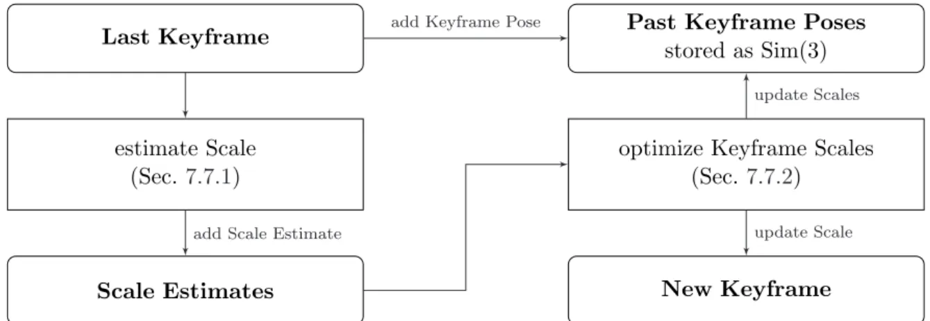
7.7 Optimizing Global Scale . . . 88
7.7.1 Keyframe based Scale Estimation . . . 88
7.7.2 Scale Optimization . . . 90
CONTENTS ix
7.8 Finding Micro Lenses of Interest . . . 90
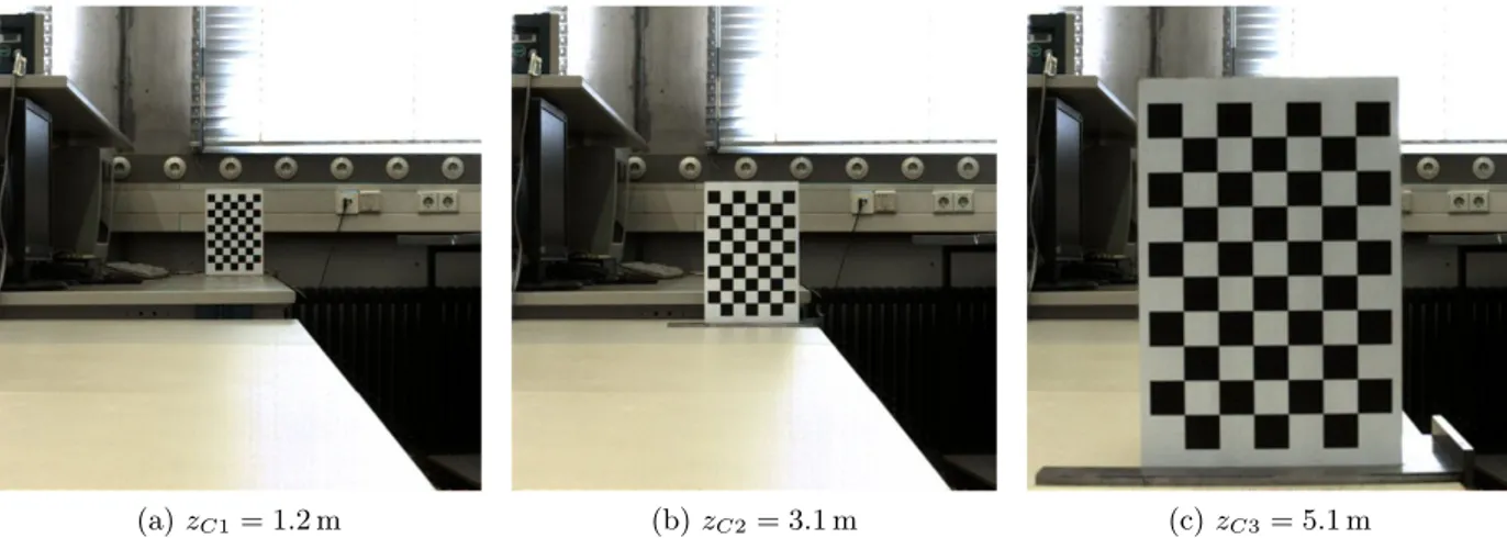
8 Experiments – Probabilistic Light Field based Depth Estimation 93 8.1 Data . . . 93
8.1.1 Checkerboard Recorded by the Plenoptic Camera Raytrix R5 . . . 93
8.1.2 Plenoptic Images of Real Scenes . . . 93
8.2 Results. . . 96
8.2.1 Quantitative Results . . . 96
8.2.2 Qualitative Results . . . 98
8.3 Conclusion . . . 101
9 Experiments – Plenoptic Camera Calibration 107 9.1 Data . . . 107
9.1.1 Series of Range Measurements . . . 107
9.1.2 Recordings of 3D Calibration Target . . . 108
9.2 Results. . . 109
9.2.1 Depth Conversion Functions. . . 110
9.2.2 Bundle Adjustment based Plenoptic Camera Calibration . . . 111
9.3 Conclusion . . . 116
10 Experiments – Full-Resolution Direct Plenoptic Odometry 119 10.1 Data . . . 119
10.1.1 Data Acquisition Setup . . . 119
10.1.2 A Synchronized Stereo and Plenoptic Visual Odometry Dataset . . . 120
10.2 Results. . . 128
10.2.1 Quantitative Results . . . 129
10.2.2 Qualitative Results . . . 134
10.3 Conclusion . . . 140
11 Summary and Prospects 141 11.1 Summary . . . 141
11.2 Future Work . . . 142
A Light Field based Depth Estimation 147 A.1 Relationship between Virtual Depth and Focus Parameter of Hog et al. [2017] . . . 147
B Direct Plenoptic Odometry 149 B.1 Pseudo Code of the DPO Algorithm . . . 149
B.2 Recursive Solution of the Global Scale Estimator . . . 151
B.3 Results from the Stereo and Plenoptic VO Dataset . . . 152
B.4 Trajectories Estimated by DPO . . . 153
Bibliography 159
Acknowledgments 167
Curriculum Vitae 169
List of Figures
1.1 Different light field sensors . . . 2
2.1 Visualization of the plenoptic function . . . 7
2.2 Two plane parametrization of a 4D light field . . . 9
2.3 Different setups to acquire 4D light fields . . . 10
2.4 Setup inside of an unfocused plenoptic camera . . . 11
2.5 Setup inside of a focused plenoptic camera . . . 12
2.6 4D light field visualizations . . . 13
2.7 Cross section of a focused plenoptic camera in the Galilean mode . . . 14
2.8 Depth estimation in a focused plenoptic camera based on the Galilean mode . . . . 16
2.9 Visualization of the tangent space of a smooth manifold . . . 18
4.1 Imaging process for a focused plenoptic camera in the Galilean mode . . . 38
4.2 Focused plenoptic camera interpreted as an array of pinhole cameras . . . 39
4.3 Multiple view epipolar geometry for plenoptic cameras . . . 41
4.4 Depth accuracy of plenoptic cameras based on plenoptic 1.0 and 2.0 rendering . . . 45
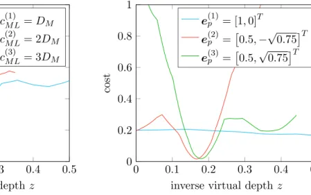
5.1 Five shortest stereo baseline distances in a hexagonal micro lens grid . . . 49
5.2 Stereo matching cost function for different baseline distances and orientations . . . 49
5.3 Visualization of the photometric disparity error . . . 53
5.4 Visualization of the focus disparity error . . . 54
5.5 Projection of a raw image point xRto a virtual image point xV . . . 55
5.6 Synthesis of the intensity value for a point in the virtual image. . . 59
5.7 Exemplary result of the probabilistic depth estimation . . . 61
6.1 Relationship between micro image and micro lens centers . . . 72
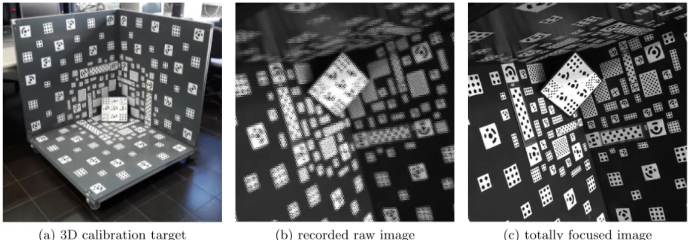
6.2 3D target used for plenoptic camera calibration . . . 73
6.3 Single calibration marker mapped to multiple micro images. . . 74
7.1 Workflow of the Direct Plenoptic Odometry (DPO) algorithm . . . 80
7.2 Keyframe depth maps and intensity images. . . 82
7.3 Tracking residual after various numbers of iterations . . . 86
7.4 Workflow of the scale optimization framework . . . 88
8.1 Checkerboard dataset recorded by a Raytrix R5 camera. . . 94
8.2 Own focused plenoptic camera dataset recorded by a Raytrix R5 camera . . . 94
8.3 Focused plenoptic camera dataset published by Hog et al. [2017] . . . 95
8.4 Raytrix R11 dataset. . . 95
8.5 Virtual depth maps calculated for the checkerboard dataset . . . 97
8.6 Virtual depth histograms of unfiltered virtual depth maps . . . 98
8.7 Results for our own Raytrix R5 dataset . . . 99
8.8 Results for the Raytrix R5 dataset of Hog et al. [2017] . . . 100 xi
8.9 Processed raw image of the “Lion” dataset of Hog et al. [2017] . . . 101
8.10 Results for the Raytrix R11 dataset . . . 102
8.11 Further results for the Raytrix R11 dataset . . . 103
8.12 Estimation uncertainty obtained by our depth estimation algorithm . . . 104
9.1 Setups for plenoptic camera calibration . . . 108
9.2 Raw image samples showing a checkerboard pattern used for the calibration method of Bok et al. [2017] . . . 109
9.3 Estimated depth conversion functions . . . 110
9.4 Depth accuracy of a focused plenoptic camera for different model parameters and camera setups . . . 113
9.5 Reprojection error map with and without the consideration of pixel distortion . . . 116
9.6 Position offset between camera model without and with squinting micro lenses . . . 117
10.1 Handheld platform to acquire time synchronized image sequences from a focused plenoptic camera and a stereo camera system . . . 119
10.2 White balance filter used to record white images for the plenoptic camera and the stereo camera system . . . 122
10.3 Estimated attenuation image for the plenoptic camera . . . 123
10.4 Estimated attenuation images for the left camera of the stereo camera system . . . 124
10.5 Semi-dense point cloud generated by DPO overlaid with the ground truth loop closure trajectory . . . 125
10.6 Sample images for one sequence of the stereo and plenoptic VO dataset . . . 126
10.7 Example sequence of the stereo and plenoptic VO dataset . . . 127
10.8 Example of the drift accumulated by DPO over an entire sequence . . . 127
10.9 Measured absolute scale errors d′s and scale driftse′s . . . 130
10.10 Measured and optimized scale for DPO as a function of the keyframe index. . . 132
10.11 Measured rotational drift and alignment error . . . 133
10.12 Sample images of sequence #5 recorded by the plenoptic camera and the stereo camera . . . 134
10.13 Comparison of point clouds received from DPO and LSD-SLAM . . . 135
10.14 Comparison of image details for the plenoptic and the monocular camera . . . 135
10.15 Point cloud reconstructed by DPO with different thresholds on the inverse effective depth variance . . . 136
10.16 Complete trajectory and point cloud calculated by DPO for a scene with abundant vegetation . . . 136
10.17 Point cloud of a hallway reconstructed by DPO . . . 137
10.18 Point clouds of stairways reconstructed by DPO . . . 138
10.19 Samples of the point clouds calculated by DPO . . . 139
B.1 Top views of the trajectory of sequence #1 . . . 153
B.2 Top views of the trajectory of sequence #2 . . . 154
B.3 Top views of the trajectory of sequence #3 . . . 154
B.4 Top views of the trajectory of sequence #4 . . . 155
B.5 Top views of the trajectory of sequence #6 . . . 155
B.6 Top views of the trajectory of sequence #7 . . . 156
B.7 Top views of the trajectory of sequence #9 . . . 156
B.8 Top views of the trajectory of sequence #10 . . . 157
B.9 Top views of the trajectory of sequence #11 . . . 157
List of Tables
8.1 Inverse virtual depth statistics obtained from the checkerboard dataset . . . 96 9.1 Estimated intrinsic camera parameters and reprojection errors . . . 112 9.2 Accuracy of 3D object coordinates estimated during the bundle adjustment . . . . 112 9.3 Robustness of the estimated intrinsic camera parameters . . . 114 10.1 Camera specifications for the plenoptic camera and the stereo camera system . . . 120 B.1 All results from the stereo and plenoptic VO dataset . . . 152 B.2 Path lengths for all sequences in the stereo and plenoptic VO dataset . . . 152
xiii
Abbreviations
1D one dimensional . . . .18
2D two dimensional . . . .2
2PP two plane parametrization . . . .8
3D three dimensional . . . .1
4D four dimensional . . . .2
AWGN additive white Gaussian noise . . . .48
CNN convolutional neural network . . . .28
CPU central processing unit . . . .31
DFT discrete Fourier transform . . . .26
DOF depth of field . . . .11
DPO Direct Plenoptic Odometry . . . .34
DSLR digital single-lens reflex DSO Direct Sparse Odometry . . . .129
EGI extended Gaussian image . . . .32
EKF extended Kalman filter . . . .30
EPI epipolar plane image. . . .13
FIR finite impulse response . . . .90
FOV field of view . . . .44
GPS Global Positioning System GPU graphics processing unit . . . .31
ICP Iterative Closest Point . . . .32
IMU inertial measurement unit . . . .33
log-scale logarithmized scale . . . .89
LRF laser rangefinder . . . .64
MAE maximum absolute error . . . .112
MLA micro lens array . . . .2
MVG multiple view geometry . . . .3
PCA principal component analysis . . . .28
RGB red, green, blue RGB-D red, green, blue - depth RMS root mean square . . . .111
RMSE root mean square error . . . .111 xv
SfM structure from motion . . . .29
SGM Semi-Global Matching . . . .129
SLAM simultaneous localization and mapping . . . .1
SNR signal to noise ratio . . . .60
SSID sum of squared intensity differences . . . .81
TCP total covering plane. . . .51
UAV unmanned aerial vehicle . . . .1
VO visual odometry . . . .2
1 Introduction
1.1 Motivation
The sense of vision allows us humans to navigate in any kind of environment without interacting with it. Furthermore, we are able to build a three dimensional (3D) map of the surroundings in our brain, based on what we see. In this way vision, in combination with other senses, enable us to navigate through and interact with our environment. In the century of automation, where we want to build autonomous cars, self-navigating unmanned aerial vehicles (UAVs) as well as mobile and intelligent robots, teaching a computer the sense of vision became a very important and broadly studied field both in research and industry. Aside from its use in automation, 3D vision can also be used to assist for instance visually impaired and elderly people in order to enhance their quality of life.
For some of the mentioned tasks, like localizing a car on an existing road map, external infrastructure can be established to achieve this goal. However, this is not always possible.
Inaccuracies in existing maps or even the lack of maps are examples of such cases. Furthermore, it might be difficult to keep maps of transient environments (e.g. moving objects and people) updated. Depending on the application, establishing such an infrastructure might simply be too expensive. Therefore, even though various systems which allow localization on a global and local scale already exist, a growing demand for closed systems which do not rely on any infrastructure for navigation and mapping can be observed.
Such tasks based on closed systems can be summarized under the research topic of simultaneous localization and mapping (SLAM). This means that a computer-based movable system is able to build a map, usually in 3D, of the environment and to localize itself within this map. Further- more, tracking and mapping are supposed to be performed online since the resulting map and trajectory have to be used e.g. for obstacle avoidance.
Depending on the application, the SLAM problem can be tackled by incorporating many different active and passive sensors, which balance each other’s capabilities and thereby are able to compensate for the failure of individual sensors. Furthermore, autonomous cars can combine the information gained through their own sensor system with that of external infrastructure like GPS(Global Positioning System). However, there are other applications where the number, size, and weight of the sensors as well as the power consumption matters. UAVs and small household robots for instance can only carry a limited weight. Furthermore, for indoor scenarios there usually are no external localization systems available and existing maps are not detailed enough and outdated since they generally do not include furniture, etc. Similar concerns hold true for assistance devices, which at best are so small and light that they are almost invisible. Besides, it is crucial that such devices operate reliably both indoors and outdoors and therefore must not be dependent on external systems. Furthermore, while some active sensors (e.g. structured light sensors) perform reliably in indoor environments with artificial lighting, they completely fail in sunlight conditions.
1
source:futurezone.at
(a) Lytro camera (1. generation) (b) Raytrix R5 camera
source:PelicanImaging
(c) PiCam, Pelican Imaging
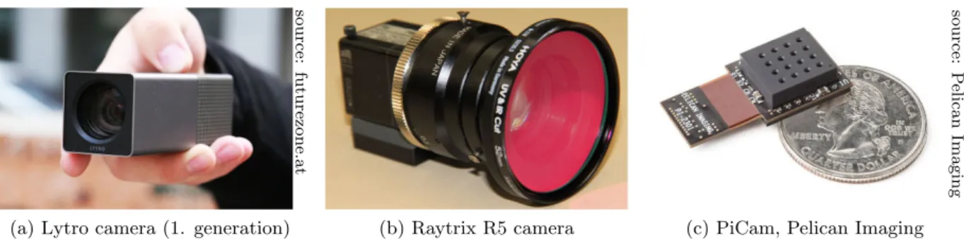
Figure 1.1: Different light field sensors. While (a) and (b) are both micro lens array based plenoptic cameras, (c) is a miniaturized 4×4 camera array.
In these scenarios, where weight and power consumption matter, theSLAMproblem is gener- ally solved based on a single monocular camera. A monocular camera captures only two dimen- sional (2D) images of the 3D world. Therefore, a 3D map can not be build without observing the scene multiple times from different perspectives. Since no absolute depth can be measured using a monocular camera, tracking and mapping can only be performed up to an unknown scale factor.
Over the last few decades, plenoptic cameras, which are also called light field cameras, with a size comparable to standard industry cameras have emerged (Adelson and Wang [1992]; Ng et al. [2005]; Lumsdaine and Georgiev [2009]; Perwaß and Wietzke [2012]) and were developed up to a commercial stage. Unlike monocular cameras, which record a 2D image of a scene, plenoptic cameras capture the light field of a scene as a four dimensional (4D) function in a single image. The additional information in two angular dimensions allows the reconstruction of the 3Dscene from a single image to a certain degree, and therefore to measure the absolute scale of a scene. Figure 1.1 shows three different, portable light field sensors. While the cameras from Lytro and Raytrix are plenoptic cameras which gather angular information based on a micro lens array (MLA) in front of the image sensor, the PiCam from Pelican Imaging is a miniaturized camera array. Here, an array of 4×4 cameras is realized on a single image sensor.
In plenoptic cameras the additional angular information is obtained at the expense of spatial resolution. However, as pixel sizes continue to shrink (currently around 1µm) and image resolu- tions of over 40 million pixels on a sensor of about 17 mm×17 mm in size can be manufactured, it seems to be a good compromise to reduce spatial resolution in order to gain additional infor- mation about the environment. This claim is supported byEngel et al. [2016] who showed that, at least for direct SLAMapproaches, increasing the image resolution does not necessarily lead to more accurate tracking results.
The motivation of this work was to study the pros and cons of plenoptic cameras with respect to visual odometry (VO) and SLAM. One question in particular, which is hoped to be answered within the context of this work, was whether or not the absolute scale of a scene can be recovered from a sequence of plenoptic images. It was also supposed to be examined whether the additional angular information gained by a plenoptic camera leads to improved tracking capabilities in comparison to monocular cameras.
In this dissertation often the two terms SLAM and VO are used to describe at first glance the same task. However, these tasks are different by definition. VO is the task of estimating the motion and therefore the trajectory of a camera (or multiple cameras) based on the recorded images. SLAMfurthermore establishes a map of its environment which aims for global consistency.
Hence, a SLAMsystem stores map information of previously explored regions and will recognize
1.2. OBJECTIVES 3
these regions when they are revisited. This is called loop closure. A VO system stores only transient map information since it is needed to estimate the camera trajectory. Therefore, loop- closures will not be recognized.
1.2 Objectives
The objective of this dissertation is to explore plenoptic cameras, built on the basis of standard industrial cameras, with respect to the task of 3D tracking and mapping and evaluate the suit- ability of these cameras for applications such as robot navigation or vision assistance for visually impaired persons.
The overarching goal of this dissertation can therefore be stated as the development and investigation of a plenoptic camera based 3D tracking and mapping algorithm. This problem is supposed to be solved by way of an example for a focused plenoptic camera by the manufacturer Raytrix (model R5). While the previous sentences define this work’s intent entirely, there are a number of secondary problems that arise on the way to achieving this goal.
One can consider the problem of camera calibration as solved for monocular cameras and stereo cameras. So far, this is not the case for plenoptic cameras. Hence, one goal was to solve the problem of plenoptic camera calibration while simultaneously finding a mathematical model for the camera that is suitable for a multiple view system.
On the basis of the camera model, tracking and depth estimation algorithms, which are able to process sequences of plenoptic images, had to be developed and combined in a plenoptic camera basedVOframework.
1.3 Dissertation Overview
Following the introduction, Chapter 2 introduces some fundamentals with respect to light field imaging as well as visual SLAM. This dissertation combines these two topics which have been handled as two more or less independent fields of research so far. Mathematical terms which are needed throughout this dissertation will be defined.
Chapter 3 gives an overview about related work and the state-of-the-art in the field of this thesis. Publications are divided into the categories of light field based depth estimation, plenoptic camera calibration, andVO(or visualSLAM). Furthermore, the main contributions of this thesis with respect to the state-of-the-art are listed.
Chapter 4 investigates the plenoptic camera from a mathematical perspective. A new math- ematical model for MLA based light field cameras is introduced. Based on this mathematical model a multiple view geometry (MVG) can be defined directly for the micro images recorded by the camera. Furthermore, the two concepts of focused and unfocused plenoptic cameras are investigated with respect to the task of depth estimation.
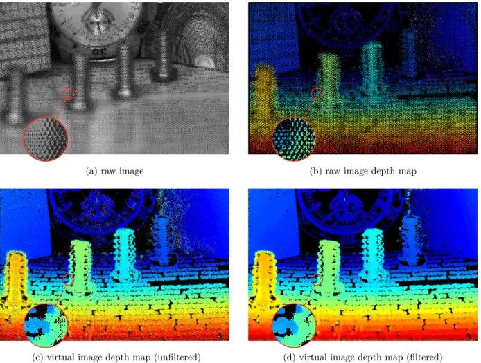
Chapter 5 introduces a probabilistic depth estimation algorithm based on a single recording of a focused plenoptic camera. The algorithm performs depth estimation without any metric calibration of the plenoptic camera. Multiple depth observations are incorporated into a single depth estimate based on a probabilistic model. A filtering method is presented to refine the probabilistic depth map. Based on this refined depth map a so called totally focused image of the recorded scene can be synthesized.
Chapter 6 presents intrinsic camera models and calibration approaches for focused plenoptic cameras on different abstraction levels. In a first model, the camera is considered to follow a
pinhole camera model, while the estimated virtual depth is transformed into object distances based on a depth conversion function. In a second model, the projection from object space to the image created by the main lens is defined. Here, in addition to lateral distortion a depth distortion model has to be defined, since depth estimation is performed prior to any image correction. The last model defines the plenoptic camera in the most complete way. It defines the projection of a 3Dobject point to multiple micro images on the sensor. Since distortion is applied directly to the recorded raw image, it is no longer necessary to consider any depth distortion.
Chapter 7 formulates a direct and semi-dense VO algorithm based on a focused plenoptic camera. This algorithm combines the mathematical plenoptic camera model and multiple view geometry (Chapter 4), the probabilistic depth estimation (Chapter 5) and the metric camera calibration (Chapter 6).
Chapter 8, Chapter 9, and Chapter 10 present the experiments which were performed to evaluate the methods developed in this thesis. To evaluate the probabilistic depth estimation algorithm two public datasets as well as light field images recorded by us are used. For the plenoptic camera calibration there are no suitable public datasets available. The used dataset was recorded based on a3Dcalibration target. Similarly, up to now there exist no public datasets for light field based VO. Therefore, a synchronized dataset was recorded to compare light field based VOwith VO algorithms relying on other sensors. The results obtained for the proposed methods based on the datasets are presented and extensively discussed.
Chapter11 summarizes this dissertation and presents prospects for further improvements and future work.
1.4 Publications
Parts of the thesis have been published in the following journal articles and conference papers:
1. Zeller N, Quint F, and Guan L (2014a). Hinderniserkennung mit Microsoft Kinect. In 34.
Wissenschaftlich-Technische Jahrestagung der DGPF (DGPF Tagungsband 23 / 2014).
2. Zeller N, Quint F, and Guan L (2014b). Kinect based 3D Scene Reconstruction. In Inter- national Conference on Computer Graphics, Visualization and Computer Vision (WSCG), volume 22, pages 73–81.
3. Zeller N, Quint F, and Stilla U (2014c). Applying a Traditional Calibration Method to a Focused Plenoptic Camera. In BW-CAR Symposium on Information and Communication Systems (SInCom).
4. Zeller N, Quint F, and Stilla U (2014d). Calibration and Accuracy Analysis of a Focused Plenoptic Camera. ISPRS Annals of Photogrammetry, Remote Sensing and Spatial Infor- mation Sciences (Proc. PCV 2014), II-3:205–212.
5. Zeller N, Quint F, and Stilla U (2014e). Kalibrierung und Genauigkeitsuntersuchung einer fokussierten plenoptischen Kamera. In 34. Wissenschaftlich-Technische Jahrestagung der DGPF (DGPF Tagungsband 23 / 2014).
6. Zeller N, Quint F, Zangl C, and Stilla U (2014f). Edge Segmentation in Images of a Fo- cused Plenotic Camera. InInternational Symposium on Electronics and Telecommunications (ISETC), pages 269–272.
1.5. COLLABORATIONS 5
7. Zeller N, Quint F, and Stilla U (2015a). Establishing a Probabilistic Depth Map from Focused Plenoptic Cameras. In International Conference on 3D Vision (3DV), pages 91–
99.
8. Zeller N, Quint F, and Stilla U (2015b). Filtering Probabilistic Depth Maps Received from a Focused Plenoptic Camera. InBW-CAR Symposium on Information and Communication Systems (SInCom).
9. Zeller N, Quint F, and Stilla U (2015c). Narrow Field-of-View Visual Odometry based on a Focused Plenoptic Camera.ISPRS Annals of Photogrammetry, Remote Sensing and Spatial Information Sciences (Proc. PIA 2015), II-3/W4:285–292.
10. Vasko R, Zeller N, Quint F, and Stilla U (2015). A Real-Time Depth Estimation Approach for a Focused Plenoptic Camera. In Advances in Visual Computing (Proc. ISVC 2015), volume 9475 ofLecture Notes in Computer Science, pages 70–80.
11. Zeller N, Noury CA, Quint F, Teuli`ere C, Stilla U, and Dhˆome M (2016a). Metric Calibra- tion of a Focused Plenoptic Camera based on a 3D Calibration Target. ISPRS Annals of Photogrammetry, Remote Sensing and Spatial Information Sciences (Proc. ISPRS Congress 2016), III-3:449–456.
12. Zeller N, Quint F, and Stilla U (2016b). Depth Estimation and Camera Calibration of a Focused Plenoptic Camera for Visual Odometry. ISPRS Journal of Photogrammetry and Remote Sensing, 118:83 – 100.
13. Zeller N, Quint F, S¨utterlin M, and Stilla U (2016c). Investigating Mathematical Models for Focused Plenoptic Cameras. In International Symposium on Electronics and Telecom- munications (ISETC), volume 12, pages 301–304.
14. K¨uhefuß A, Zeller N, and Quint F (2016). Feature Based RGB-D SLAM for a Plenoptic Camera. InBW-CAR Symposium on Information and Communication Systems (SInCom), pages 25–29.
15. Konz J, Zeller N, and Quint F (2016). Depth Estimation from Micro Images of a Plenoptic Camera. InBW-CAR Symposium on Information and Communication Systems (SInCom), pages 17–23.
16. Zeller N, Quint F, and Stilla U (2017). From the Calibration of a Light-Field Camera to Direct Plenoptic Odometry. IEEE Journal of Selected Topics in Signal Processing (JSTSP), 11(7):1004–1019.
17. Zeller N, Quint F, and Stilla U (2018). Scale-Awareness of Light Field Camera based Visual Odometry. InEuropean Conference on Computer Vision (ECCV), pages 715–730.
1.5 Collaborations
Parts of this thesis have been developed in collaboration with other colleagues. The real time implementation of the probabilistic depth estimation algorithm (Vasko et al.[2015]) was done by Ross Vasko from the Ohio State University, USA, as a summer intern at Karlsruhe University of Applied Sciences. The plenoptic camera calibration approach which was published at the ISPRS Congress 2016 in Prague (Zeller et al. [2016a] (parts of Sections 6.2.1, 6.3.1, and 6.3.2)) was developed in collaboration with Charles-Antoine Noury from Institut Pascal in Clermont- Ferrand, France, during his stay in Karlsruhe.
1.6 Notations
In this section important notations, which are used throughout this dissertation, are introduced.
Matrices are denoted as bold, capital letters (G), vectors as bold, lower case letters (x) and scalars as normal letters, either capital or lower case (d). It is not differentiated between homogeneous (x= [x, y, z,1]T) and non-homogeneous (x= [x, y, z]T) representations. Nevertheless, the mean- ing should be clear from the context. The notation [t]i defines the i-th element of a vector tand [R]j the j-th row of a matrix R. The determinate of a matrix R is denoted by |R| and tr(R) denotes the trace of a matrix R.
2 Fundamentals – Light Field Imaging and Visual SLAM
2.1 The Light Field
While a regular camera captures only the amount of light hitting a 2D image sensor, the light field is what describes the entire distribution of light in a 3D volume. First explorations of the light field were made byGershun [1936], more than eighty years ago.
2.1.1 The Plenoptic Function
A general definition of the light field, as it is used today in image processing, was given by Adelson and Bergen[1991]. They described the entire distribution of light in3Dspace by a seven dimensional function which they called theplenoptic function. Here, the intensity distribution of light is defined for any point (Vx,Vy,Vz) in the3Dspace, with respect to the angle (Φ,Θ) of the respective light ray, at a certain wavelength λ, for any time t:
P(Φ, Θ, λ, Vx, Vy, Vz, t). (2.1)
source:AdelsonandBergen[1991]
Figure 2.1: Original drawing byAdelson and Bergen[1991], which is a quite famous visualization of the plenoptic function. The plenoptic function describes the amount of light penetrating any point in space (Vx,Vy,Vz) from any possible angle (Φ,Θ). This is shown here schematically with two eyes representing two different observer positions. While a real observer does not gather light rays coming from behind, these are included in the plenoptic function.
7
While there might be even more dimensions, describing, for instance, the light’s polarization, the plenoptic function stated in eq. (2.1) gives a quite generalized definition of the light field. Anyhow, as one will see in the following, several assumptions can be made with respect to computational imaging. The plenoptic function considered here will only be a subset of the function given in eq. (2.1).
When processing images, one is not interested in the absolute time t. Even for the task of visual odometry as discussed in this thesis, the assumption of a light field which is stationary, at least in a wide sense, has to be made. Furthermore, when considering a monochromatic image sensor, the plenoptic function is integrated along a certain bandwidth of the wavelength domain.
Therefore, the function will be independent of the wavelength λ itself. Hence eq. (2.1) shrinks down to a five dimensional function:
P(Φ, Θ, Vx, Vy, Vz). (2.2)
For RGB sensors one can simply consider the three colors as separate channels of the plenoptic function. The function given in eq. (2.2) can be visually interpreted as shown in Figure2.1, which is the original drawing by Adelson and Bergen [1991]. Here, the coordinates (Vx, Vy, Vz) can be considered as the position of an observer, while (Φ, Θ) are the angles corresponding to a light ray going through the observer’s pupil. While a real-eye observer would only gather the light rays coming from in front, the plenoptic function considers all rays penetrating from every direction.
Another simplification of the plenoptic function can be made when considering the intensity distribution P along a ray being independent of the absolute position along the respective light ray. This assumption holds true as long as the ray is traveling through free space without hitting any object or being attenuated by some medium. One can parametrize the light field on a surface outside the convex hull of the scene as given in eq. (2.3) (Gortler et al.[1996]).
P(Φ, Θ, x, y) (2.3)
This4D plenoptic function has its limitation in that only the light field around a scene bounded by a convex hull can be parameterized. While this assumption implies certain limitations, the4D plenoptic function represents the nature of light fields captured by common imaging systems.
2.1.2 Light Field Parametrization and Capturing
While in the previous section the plenoptic function was considered as a continuum, what we capture is just a sampled version of it, where the intensity distribution is integrated over a certain area (e.g. the photosensitive are of a sensor pixel). There are several ways to parametrize this sampled4Dlight field. The most popular one is the two plane parametrization (2PP) introduced byLevoy and Hanrahan[1996]. A ray in the 4Dlight field is defined by its intersections with two parallel planes Ω and Π, where the intersections are defined by the coordinates (u, v) ∈ Ω and (s, t)∈Π respectively:
L(u, v, s, t). (2.4)
Each ray (u, v, s, t) in the light field is described by its corresponding intensity value L. Here, it is important to notice that the variable tdoes not represent time. Figure 2.2visualizes this two plane parametrization. The figure illustrates the example of two light rays (L1 andL2) of the4D light field. Both rays are emitted from the same point O(Vx, Vy, Vz) in 3D space and therefore intersect in this point. Since both rays are emitted from the same point, they will have the same intensity value (L1=L2), as long as Lambertian reflectance is assumed.
2.2. THE PLENOPTIC CAMERA 9
L1
L2
s
t u
v
O(Vx, Vy, Vz) Π
Ω
Figure 2.2: Two plane parametrization (2PP). Light rays are defined based on their intersections with two parallel planes and have a certain intensity value L. The figure shows the example of two light raysL1 and L2 emitted from the same point O(Vx, Vy, Vz) in the3Dspace.
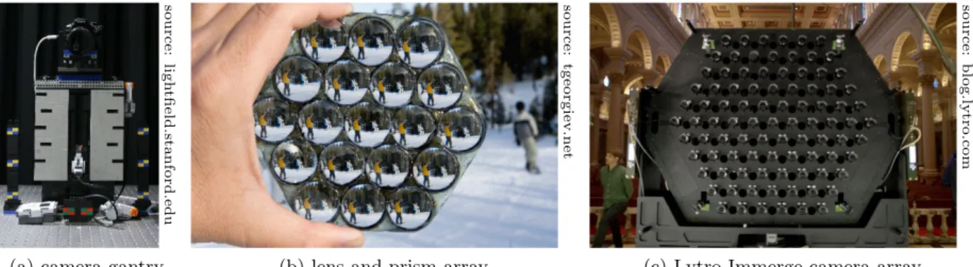
At first glance this parametrization seems to have quite a few limitations. Only the light field outside a convex hull and on a planar cut through the 3D space is covered. However, the two plane parametrization is sufficient for the data gathered by most of today’s light field capturing setups. Some of these setups are shown in Figure 2.3, which all basically form arrays of real or virtual cameras. Figure2.3ashows a gantry, which is able to capture the4Dlight field of a static scene by moving a camera in horizontal and vertical direction. Figure 2.3b shows an array of lenses and prisms, which can be used to capture a light field using a single camera. Figure 2.3c shows a large camera array, based on which high resolution light field videos of dynamic scenes can be captured.
A convenient feature of 4D light fields captured by camera arrays is that they already are recorded in a format conforming to the two plane parametrization. Consider a camera array, for instance, where all cameras are arranged on a plane and are pointing in the same direction.
The plane Ω can be defined as the plane of the camera lenses, while the plane Π defines the respective image plane. Hence, for the conventional pinhole camera model, the planeΠ is defined in distance f in front of the plane Ω, where f is the cameras’ focal length. Selecting certain coordinates (u, v) on the planeΩis equivalent to the selection of a certain camera in the array. In contrast selecting coordinates (s, t) would be equivalent to the selection of a respective pixel in the rectified images. Even though both coordinates (u, v) and (s, t) define positions on the respective plane, the coordinates (s, t) are referred to as spatial coordinates while (u, v) are referred to as angular coordinates. The coordinates (s, t) define the spatial samples in a single image of the camera array, while the coordinates (u, v) define the position of the respective pinhole camera and hence the viewing angle on the scene.
2.2 The Plenoptic Camera
For camera arrays it is quite intuitive to see that they capture a 4D light field which conforms to the two plane parametrization. However, it is not as obvious that a MLA based light field camera, as drawn in Figure2.4, does so, too.
In this section we will discuss both concepts ofMLAbased light field cameras: the traditional, unfocused plenoptic camera (or plenoptic camera 1.0) proposed byAdelson and Wang[1992] and
source:lightfield.stanford.edu
(a) camera gantry
source:tgeorgiev.net
(b) lens and prism array
source:blog.lytro.com
(c) Lytro Immerge camera array
Figure 2.3: Different setups to acquire 4D light fields. (a) Stanford’s Lego Mindstorms gantry.
Here an assembled DSLR camera can be moved in horizontal and vertical direction to capture images from different viewpoints on a plane. (b) Optical device byGeorgiev et al.[2006] consisting of 19 lenses and 18 prisms. It can be placed in front of a regular camera lens to capture4Dlight fields. (c) Lytro Immerge. Large camera array to capture 4Dlight field videos in cinema quality.
developed further byNg et al.[2005] and the focused plenoptic camera (or plenoptic camera 2.0) introduced byLumsdaine and Georgiev[2009] and commercialized byPerwaß and Wietzke[2012].
2.2.1 The Unfocused Plenoptic Camera
There are different ways to look at plenoptic cameras. In contrast to the perspective presented here, there are plenty of other ways to describe the concept of plenoptic imaging (e.g. Dansereau [2013] (Sec. 2.3)). Here, the plenoptic camera is considered to be an array of cameras that captures the light field inside the camera and therefore behind the main lens. As will be shown in the following, this light field conforms to the two plane parametrization. Hahne et al. [2014]
show how this array can be transformed into an array outside the camera. However, here the data conforms to the two plane parametrization only under certain conditions.
For an unfocused plenoptic camera, the focal length fM of the micro lenses is chosen to be equal to the distance B between sensor andMLA(see Fig.2.4). Thus, each micro lens is focused to infinity and thus each pixel under a micro lens integrates intensities over a bundle of rays which incident in parallel on the micro lens. For the light field parametrization one plane of the two plane parametrization can be chosen to be theMLAplane, where each micro lens is one sample, while the second plane is the main lens plane sampled by the pixels under a micro lens. Hence, the plane Ω is defined to be on theMLAand the planeΠ on the main lens.
This setup of the unfocused plenoptic camera is shown in Figure2.4. As one can see from the figure, each micro lens gathers light across the complete aperture of the main lens, while each pixel under the micro lens captures only rays from a small sub-aperture. From the previous section one can remember that picking a point (u, v) on the plane Ωcan be considered as selecting a specific camera from the camera array, while the central perspective image of this camera is formed on the plane Π. This can be done in a similar way for the plenoptic camera. By selecting a point (u, v) one chooses a certain sub-aperture on the main lens and respectively a certain pixel position under the micro lenses. Hence, by arranging the pixels with certain coordinates from each micro image in an array, according to the corresponding micro lens position (s, t), again, a central perspective view is obtained (see Figure 2.6a). This is a simplified perspective on the image recorded by a plenoptic camera, where it is assumed that theMLAconsists of rectangular micro lenses and each micro image consists of an integer number of pixels. For real data, interpolation and resampling have to be performed. However, the principle of the concept is as stated.
2.2. THE PLENOPTIC CAMERA 11
main lens sensor MLA
image plane
B =fM bL0
Figure 2.4: Setup inside of an unfocused plenoptic camera. While each micro lens captures light penetrating the whole of the main lens aperture (shown in blue), a single pixel on the sensor only gathers a bundle of rays penetrating a small subsection of the main lens aperture.
In this thesis, plenoptic cameras are mainly considered from a geometric perspective. But for interested readers who seek further insight into the topic of plenoptic imaging, the author would like to refer them to the work of Dansereau [2013]. In his PhD thesis (Dansereau [2013], Section 2.3), he compares a traditional camera to a plenoptic camera with respect to the captured depth of field (DOF) as well as the amount of light which is gathered.
2.2.2 The Focused Plenoptic Camera
One limitation of unfocused plenoptic cameras is that the spatial resolution, i.e. the resolution of the planeΩin the2PP, is limited by the number of micro lenses in theMLA. The idea behind the focused plenoptic camera or plenoptic camera 2.0 is to find an imaging concept which decouples this connection and therefore adds more degrees of freedom to the design of a plenoptic camera.
Instead of placing theMLAin the image plane of the main lens, it is placed either in front of or behind that image plane. Furthermore, the micro lenses are not focused at infinity, but at the image plane of the main lens. This is shown in Figure2.5for an image plane in front of theMLA, called Keplerian mode (Figure2.5a), and an image plane behind the MLA, called Galilean mode (Figure2.5b). A micro lens with focal length fM < B has to be chosen for the Keplerian mode and fM > B for the Galilean mode. More precisely, for the Keplerian mode the micro lens focal length is given by
fM = b·B
b+B, (2.5)
while for the Galilean mode a micro lens focal length of fM = b·B
b−B (2.6)
results from the thin lens equation. While in the Keplerian mode a real main lens image is formed and captured by theMLA, the image of the main lens in the Galilean mode exists only as virtual image behind the image sensor.
In the setup of a focused plenoptic camera, the micro images are focused subsections of the main lens image. Hence, this main lens image plane is sampled with a spatial resolution which is decoupled from the number of micro lenses in the MLA. Instead, the spatial resolution on the image plane is defined by the ratio Bb and the pixel pitch. Increasing the distancebbetween image plane and MLA will decrease the spatial resolution, while reducing the distance will increase it accordingly. At the same time that the spatial resolution is increased, the number of angular
main lens sensor
MLA
B
bL0
b bL
image plane
(a) Keplerian configuration
main lens sensor
MLA
B
bL0 b
bL image plane
(b) Galilean configuration
Figure 2.5: Setup inside of a focused plenoptic camera. (a) Keplerian configuration: the image plane of the main lens is in front of the MLA. (b) Galilean configuration: the image plane of the main lens is behind the MLA. In both cases the micro lens’ focal lengths are matched such that the main lens image is focused on the sensor. In this schematic drawing aperture matching between micro lenses and main lens was not considered.
samples decreases, since an image point is seen by fewer micro lenses. Thus, since the total number of rays is given by the number of sensor pixels, a tradeoff between spatial and angular resolution has to be found. This phenomena was discussed exhaustively byGeorgiev et al.[2006].
Assuming Bb = 1, for instance, would imply that each image point is seen by only a single micro lens. Therefore, for each image point there would exist only one angular sample, while the spatial domain is sampled at full sensor resolution. For this case the focused plenoptic camera would, in theory, act as the equivalent of a monocular camera.
Similar to the way that the number of captured light rays is directly coupled to the number of pixels on the sensor, the depth of field (DOF) captured by the camera is coupled to the angular resolution. Hence, increasing the spatial resolution will result in a decreasedDOF in comparison to the equivalent unfocused plenoptic camera.
In conclusion, the main difference between an unfocused and a focused plenoptic camera is the manner of sampling. In an unfocused plenoptic camera, theMLAsamples the spatial domain of the light field and the sensor pixels sample the angular domain. In the case of the focused plenoptic camera, the reverse is true. Generally speaking, an unfocused plenoptic camera exhibits more vagueness in the spatial domain, while a focused plenoptic camera exhibits more vagueness in the angular domain. This can also be seen when considering the ray bundle of a single pixel in Figure 2.4and Figure 2.5, respectively.
With regards to the2PP, the unfocused plenoptic camera already samples the light field in a uniform fashion, whereas the focused plenoptic camera performs a nonuniform sampling of the light field, which cannot be arranged directly in an equally spaced 2PP. Therefore, obtaining a uniformly sampled 2PP from a focused plenoptic camera requires depth estimation and interpo- lation of the light field (Wanner et al. [2011]).
A further extension to the focused plenoptic camera is the multi-focus plenoptic camera pro- posed byPerwaß and Wietzke[2012]. Here aMLAconsisting of different interlaced types of micro lenses is used. Each micro lens type has a different focal length and therefore is focused on a different image plane. This way the lost depth of field can be compensated for, to some degree.
2.3. VISUALIZATIONS OF 4D LIGHT FIELD RECORDINGS 13
(a) sub-aperture images (b) center sub-aperture image andEPIs
Figure 2.6: 4D light field visualizations. (a) Sub-aperture images: each image corresponds to a specific sample (u, v) on the plane Ω and hence is showing the scene from a slightly different perspective. (b) Epipolar plane images (EPIs): top and right part show slices through the (v, t) and (u, s) domain of the light field respectively. The resultingEPIs represent a point of the scene as a straight line of constant color. Here, the slope of the line is directly correlated to the depth of the scene point. The image in the center shows the central sub-aperture image. The light field was resampled from the recoding of a Lytro camera using the methods ofDansereau et al.[2013].
However, this setup makes the interpretation of the recorded data in the sense of a4Dlight field even more complicated.
2.3 Visualizations of 4D Light Field Recordings
There are mainly two popular ways to visualize recorded4Dlight fields. They will be discussed in the following. These are the so-calledsub-aperture images and theepipolar plane images (EPIs).
Both visualizations represent the light field as a set of2D functions and therefore as a set of 2D slices through the two plane parametrization (2PP).
The sub-aperture images are the most obvious visualization of light fields. As discussed before, selecting coordinates (u, v) on the plane Ω in the 2PP can be interpreted as picking a pinhole camera located on this plane. The sub-aperture images are simply the images of these pinhole cameras and thus2Dslices along the planeΠ. Figure2.6ashows the sub-aperture images extracted from a Lytro camera. Here, each of the images shows the same scene from a slightly different perspective and hence from different coordinates (u, v). Since each image is captured through only a subsection of the complete aperture, each image by itself has a very large depth of field. The set of sub-aperture images represent the complete 4D light field. This set can be used for disparity estimation and to synthesize a single full aperture image focused at different focal planes.
Figure 2.6b exemplary shows two EPIs as well as the center sub-aperture image. The EPIs represent slices along the (u, s) and (v, t) domains of the 2PP, respectively. As one can see from the figure, a single point in the 3D space corresponds to a straight line of constant color in the
B bL0 b
fL fL
bL zC
DM
DM DM
DL
main lens sensor
MLA
Figure 2.7: Cross section of a focused plenoptic camera in the Galilean mode. Main lens creates a virtual image of a real object behind the sensor. The virtual image is captured in multiple micro images on the sensor.
EPI. The distance of this point is encoded in the slope of the line. Let us consider a point lying on the plane Π, for instance. All rays corresponding to this point have the same coordinates s and t, respectively, while u and v can be swept across the entire range. Therefore, a point lying on the plane Π will result in a line of constant color which is perpendicular to the sand t axis, respectively. A point lying between the two planes Ω andΠ will result in a negative slope along the u and v axis respectively, while a point behind the plane Π (referred to Ω) will result in a positive slope.
Considering this depth encoding in the2PP, disparity estimation from the light field can be considered as the estimation of the slope of lines of constant color through the EPI(Wanner and Goldl¨ucke [2014]), while image refocusing can be performed by shearing theEPIs and integrating along the (u, v) domains.
2.4 Depth Estimation for Plenoptic Cameras
This thesis deals with light fields captured by focused plenoptic cameras. Therefore, the idea of depth estimation is discussed exclusively for this type of camera. Depth estimation from the image of an unfocused plenoptic camera can be considered either as finding pixel correspondences in the set of sub-aperture images (e.g. Jeon et al. [2015]) or as estimating the slope of straight lines of constant color in theEPIs (e.g. Wanner and Goldl¨ucke[2012]). The first task basically can be solved by standard stereo matching algorithms since the sub-aperture images form a multiple view stereo configuration. However, disparities have to be estimated with sub-pixel accuracy due to the small stereo baselines.
As discussed before, the light fields captured by focused plenoptic cameras do not conform to a uniformly sampled2PP. Hence, sub-aperture images can not be extracted directly. Instead, the task of depth estimation is solved by finding pixel correspondences directly in the recorded micro images. In the following, the concept of depth estimation is described for the Galilean mode.
However, it can be applied in a similar way to the Keplerian mode.
Figure2.7shows again a complete cross section of a focused plenoptic camera in the Galilean mode. The main lens produces a virtual image of an object, which is located at a distancezc in
2.4. DEPTH ESTIMATION FOR PLENOPTIC CAMERAS 15
front of the main lens, at the distance bLbehind the main lens. The relationship between image distance bL and object distancezC is defined by the thin lens equation:
1 fL
= 1 zC
+ 1 bL
. (2.7)
In general, a virtual image point is projected to multiple micro images. This can be guaranteed by placing the MLA with respect to the main lens’ focal length fL (min(bL) = fL). Since the minimum image distance min(bL) is equivalent to the main lens focal length fL, the parameter bL0 must be chosen in such a way that an image point at distance fL to the main lens is still visible in multiple micro images. Perwaß and Wietzke[2012] discuss this problem extensively for different MLAarrangements.
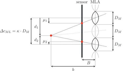
Figure2.7shows how the virtual image is projected by the three middle micro lenses onto dif- ferent pixels of the sensor. If it is known which pixels on the sensor correspond to the same virtual image point, the distanceb betweenMLAand virtual image can be calculated by triangulation.
To derive how the distance b can be calculated, Figure 2.8 shows an example of the trian- gulation for a virtual image point, based on the corresponding points in two micro images. In Figure2.8µi (fori∈ {1,2}) define the distances of the points in the micro images with respect to the principal points of their micro images. Similarly, di (fori∈ {1,2}) define the distances of the respective principal points to the orthogonal projection of the virtual image point on the MLA.
All distances µi, as well as di, are defined as signed values. Distances with an upwards pointing arrow in Figure2.8have positive values and those with a downward pointing arrow have negative values. Triangles which have equal angles are similar and therefore the following relations hold:
µi B = di
b −→ µi = di·B
b for i∈ {1,2}. (2.8)
The baseline distance∆cM L between the two micro lenses can be calculated as given in eq. (2.9).
∆cM L=d2−d1 (2.9)
The disparityµof the virtual image point is defined as the difference betweenµ2 andµ1, and the relation given in eq. (2.10) is obtained.
µ=µ2−µ1= (d2−d1)·B
b = ∆cM L·B
b (2.10)
After rearranging eq. (2.10), the distance b between a virtual image point and the MLAcan be described as a function of the baseline distance∆cM L, the distanceB betweenMLAand sensor, and the disparityµ, as given in eq. (2.11).
b= ∆cM L·B
µ (2.11)
The number of micro images in which a virtual image point will appear depends on its distance bto theMLA. Thus, the length of the longest baseline∆cM L, which can be used for triangulation, changes. It can be defined as a multiple of the micro lens diameter ∆cM L = κ·DM (κ ≥ 1).
Here, κ is not necessarily an integer, due to e.g. the 2Darrangement of the micro lenses in the MLA. Instead, for a hexagonally arranged MLA, which is the case for most plenoptic cameras, the first 10 values ofκ are as follows: 1.00, 1.73, 2.00, 2.65, 3.00, 3.46, 3.61, 4.00, 4.36, 4.58.
The baseline distance∆cM Land the disparityµare both defined in pixels and can be measured from the recorded micro lens images, while the distance B betweenMLA and sensor is a metric
µ1
µ2 d1
d2
∆cM L=κ·DM
DM
DM
DM
B b
sensor MLA
Figure 2.8: Depth estimation in a focused plenoptic camera based on the Galilean mode. The distance bbetween a virtual image point and theMLAcan be calculated based on its projection in two or more micro images.
dimension which cannot be measured precisely. Thus, the distance b is estimated relatively to the distance B. This relative distance, which is free of any unit and is called virtual depth, will be denoted by v throughout this thesis:
v= b
B = ∆cM L
µ . (2.12)
To retrieve the real depth, i.e. the object distance zC between an observed point and the camera, one has to estimate the relation between the virtual depth v and the image distance bL (which relies on B and bL0) in a calibration process. Then, one can use the thin lens equation (eq. (2.7)) to calculate the object distancezC.
Once the virtual depthv has been estimated from the micro images, one is able to project the corresponding points into the image space and therefore to reconstruct a convex surface of the virtual image, including the corresponding intensities. It will be focused on that in more detail in Chapter 5.
2.5 Visual SLAM
The task of visualSLAMis about finding the position and orientation of a camera moving through 3D space while simultaneously building a 3D map of its surroundings. This section introduces basic components ofSLAMsuch as transformations in3DEuclidean space and its representations or nonlinear optimization, which the work presented in this dissertation builds upon.
2.5.1 Rigid Body and Similarity Transformation
The orientation and position of a camera in 3Dspace can be described by a rigid body transfor- mation (or rigid body motion) which is also called a3Dspecial Euclidean transformation. Special means that reflections are excluded from the set of Euclidean transformations and therefore the respective transformation matrix has a determinate of +1. The set of all special Euclidean trans- formations in3Dis denoted by SE(3) and is also referred to as the special Euclidean group. The group of3Drotational transformations is a subgroup of the special Euclidean group SE(3).