A stochastic volatility Libor model and its robust calibration

(1)

SFB 649 Discussion Paper 2007-067

A stochastic volatility Libor model and its robust

calibration

Denis Belomestny*

Stanley Matthew**

John Schoenmakers*

* Weierstrass Institute Berlin, Germany

** Johann Wolfgang Goethe-Universität Frankfurt/Main, Germany

This research was supported by the Deutsche

Forschungsgemeinschaft through the SFB 649 "Economic Risk".

http://sfb649.wiwi.hu-berlin.de ISSN 1860-5664

SFB 649, Humboldt-Universität zu Berlin

S FB

6 4 9

E C O N O M I C

R I S K

B E R L I N

(2)

A stochastic volatility Libor model and its robust calibration

Denis Belomestny

^1,^∗

, Stanley Mathew

²

, and John Schoenmakers

¹

December 10, 2007

Keywords: Libor modelling, stochastic volatility, CIR processes, calibration AMS 2000 Subject Classification: 60G51, 62G20, 60H05, 60H10, 90A09, 91B28 JEL Classification Code: G12

Abstract

In this paper we propose a Libor model with a high-dimensional spe- cially structured system of driving CIR volatility processes. A stable calibration procedure which takes into account a given local correlation structure is presented. The calibration algorithm is FFT based, so fast and easy to implement.

1 Introduction

Since Brace, Gatarek, Musiela (1997), Jamshidian (1997), and Miltersen, Sand- mann and Sondermann (1997), almost independently, initiated the development of the Libor market interest rate model, research has grown immensely towards improved models that fit market quotes of standard interest rate products such as cap and swaption prices for different strikes and maturities. As a matter of fact, while caps can be priced using a Black type formula and swaptions via closed form approximations with high accuracy, an important drawback of the market model is the impossibility of matching cap and swaption volatility smiles and skews observed in the markets. As a remedy, various alternatives to the standard Libor market model have been proposed. They can be roughly categorized into three streams: local volatility models, stochastic volatility models, and jump-diffusion models. Especially jump-diffusion and stochastic

1Weierstrass Institute for Applied Analysis and Stochastics, Mohrenstr. 39, 10117 Berlin, Germany. {belomest,schoenma}@wias-berlin.de.

2Johann Wolfgang Goethe-Universit¨at, Senckenberganlage 31, 60325 Frankfurt am Main, Germany. mathew@math.uni-frankfurt.de.

∗partial support by the Deutsche Forschungsgemeinschaft through the SFB 649 ‘Economic Risk’ is gratefully acknowledged.

(3)

volatility models are popular due to their economically meaningful behavior, and the greater flexibility they offer compared to local volatility models for in- stance. For local volatility Libor models we refer to Brigo and Mercurio (2006).

Jump-diffusion models for assets go back to Merton (1976) and Eberlein (1998).

Jamshidian (2001) developed a general semimartingale framework for the Libor process which covers the possibility of incorporating jumps as well as stochastic volatility. Specific jump-diffusion Libor models are proposed, among others, by Glasserman and Kou (2003) and Belomestny and Schoenmakers (2006).

Levy Libor models are studied by Eberlein and ¨Ozkan (2005). Incorporation of stochastic volatility has been proposed by Andersen and Brotherton-Ratcliffe (2001), Piterbarg (2004), Wu and Zhang (2006), Zhu (2007).

In the present article we focus on a flexible particularly structured Heston type stochastic volatility Libor model that, due to its very construction, can be calibrated to the cap/strike matrix in a robust way. In this model we incorporate a core idea from Belomestny and Schoenmakers (2006), who propose a jump- diffusion Libor model as a perturbation of a given input Libor market model. As a main issue, Belomestny and Schoenmakers (2006) furnish the jump-diffusion extension in such a way that the (local) covariance structure of the extended model coincides with the (local) covariance structure of the market model. The approach of perturbing a given market model while preserving its covariance structure, has turned out to be fruitfull and is carried over into the design of the stochastic volatility Libor model presented in this paper. In fact, this idea is supported by the following arguments (see also Belomestny and Schoenmakers (2006)).

1. Cap prices do not depend on the (local) correlation structure of forward Libors in a Libor market model but, typically, do depend only weakly on this in a more general model. Since this correlation structure contains important information about, for example, prices of ATM swaptions, we do not want to destroy this (input) correlation structure while calibrating the extended model to the cap(let)-strike matrix.

2. The lack of smile behavior of a Libor market model is considered a conse- quence of Gaussianity of the driving random sources (Wiener processes).

Therefore we want to perturb this Gaussian randomness to a non-Gaussian one by incorporating a CIR volatility process, while maintaining the (local)correlation structureof the Libor market model we started with.

3. Preserving the correlation structure allows for robust calibration, since it significantly reduces the number of parameters to be calibrated while holding a realistic correlation structure.

Specifically, the perturbation part of the presented model will involve CIR volatility processes, and so the construction will finally resemble a Heston type Libor model (Heston (1993)). The CIR model, as developed by its founders Cox, Ingersoll, Ross (1985), was originally derived in a framework based on equilibrium assumptions.

(4)

The idea of utilizing a Heston type process has already been formulated in Wu and Zhang (2006), and Zhu (2007). However, the present article differs from these works in the following respects.

1. As opposed to a one-dimensional stochastic volatility process as in Wu &

Zhang, or a (possibly) vector valued one which inhibits only one source of randomness as in Zhu (2007), we will study multi-dimensional CIR vector volatility processes with each component being driven by its own Brownian motion. This leads to a more realistic local correlation structure and renders the model more flexible for calibration.

2. We suggest a multi-dimensional partial-Gaussian and partial-Heston type model, where each forward Libor is driven by a linear combination of CIR processes.

3. While in both papers the issue of robust calibration has not been ad- dressed, we give full consideration to this problem using novel ideas mentioned above.

Furthermore, approximative analytic pricing formulas for caplets and swaptions are derived for this new Libor model which allow for fast calibration to these products. Ultimately, complex structured Over The Counter products may be priced by Monte Carlo using guidelines for simulating Heston type models as given in Kahl and J¨ackel (2006).

2 Dynamics of the Libor Model

Consider a fixed sequence of tenor dates 0 =: T0 < T1 < . . . < Tn, called a tenor structure, together with a sequence of so called day-count fractions δi:=Ti+1−Ti, i= 1, . . . , n−1. With respect to this tenor structure we consider zero bond processesBi, i= 1, . . . , n,where eachBi lives on the interval [0, Ti] and ends up with its face valueBi(Ti) = 1. With respect to this bond system we deduce a system of forward rates, called Libor rates, which are defined by

Li(t) := 1 δ_i

Bi(t) B_i+1(t)−1

, 0≤t≤Ti, 1≤i≤n−1.

Note that Li is the annualized effective forward rate to be contracted at the datet, for a loan over a forward period [Ti, Ti+1]. Based on this rate one has to pay atTi+1 an interest amount of $δiLi(Ti) on a $1 notional.

For a pre-specified volatility processγi∈R^m,adapted to the filtration gen- erated by some standard Brownian motionW ∈R^m,the dynamics of the corresponding Libor model have the form,

dLi

Li

= (...)dt+γ_i^>dW (1)

i= 1, ..., n−1.The drift term, adumbrated by the dots, is known under different numeraire measures, such as the risk-neutral, spot, terminal and all measures

(5)

induced by individual bonds taken as numeraire. If the processest→γi(t) in (1) are deterministic, one speaks of a Libormarket model.

In this work we study extensions of a Libor market model, which is given via a deterministic volatility structureγ,with respect to an extended Brownian filtration. In particular, we consider extensions with the following structure,

dL_i Li

= (...)dt+ q

1−r²_iγ_i^>dW +riβ_i^>dU, 1≤i < n, (2)

dUk=√

vkdfWk 1≤k≤d, dvk=κk(θk−vk)dt+σk

√vk

ρkdfWk+ q

1−ρ²_kdWk

, (3)

where fW and W are mutually independentd-dimensional standard Brownian motions, both independent ofW. In (2),βi∈R^dare chosen to be deterministic vector functions. They will be specified later. Theri are constants that may be considered ”allotment” or ”proportion” factors, quantifying how much of the original input market model should be in play. Forr_i= 0 for alli, it is easily seen from (2) that the classical market model is retrieved. As such, for small values of ther_i,the extended model may be regarded as a perturbation of the former.

Finally, from a modeling point of view system (2) is obviously overparameterized in the following sense. By settingβ_ik=:α_kβe_ik andv_k =:α⁻²_k ve_k, θ_k =:α⁻²_k θe_k, σk =:α⁻¹_k eσk, we retrieve exactly the same model. From now on we therefore normalize by settingθk≡1 without loss of generality.

It is helpful to think of the Libor model as a vector-valued stochastic process of dimensionn−1 driven bym+ 2d standard Brownian motions with dynamics of the form

dL_i Li

= (...)dt+ Γ^>_i dW, i= 1, ..., n−1, where

Γ_i=







p1−r_i²γi1

p1−r_i²γ_i2

·

· p1−r²_iγim

r_iβ_i1√ v₁

·

· r_iβ_id√

v_d







dW=





 dW1

dW2

·

· dWm

dfW₁

·

· dfW_d







. (4)

In (4) the square-root processesv_k are given by (3) (withθ_k ≡1).

In our approach we will work throughout under the terminal measurePn. Fol- lowing Jamshidian (1997, 2001), the Libor dynamics in this measure are given

(6)

by

dLi

Li

=−

n−1

X

j=i+1

δLj

1 +δLj m+d

X

k=1

Γ_jkΓ_ik

!

dt+ Γ^>_i dW⁽ⁿ⁾. (5) Often it turns out technically more convenient to work with the log-Libor dynamics. A straightforward application of Itˆo’s lemma to (5) yields,

dlnL_i =−1

2|Γ_i|²dt−

n−1

X

j=i+1

δLj

1 +δL_j

m+d

X

k=1

Γ_jkΓ_ik

!

dt+ Γ^>_i dW⁽ⁿ⁾, 1≤i < n.

(6)

3 Reduction of parameters by covariance assump- tion

Within the particular framework constructed above, one could interpret the second diffusion part in (2), namelyriβ_i^>dU, as an extension or perturbation of a given Libor market model.

Let us integrate the diffusion part of (6) from zero totand define the resulting zero-mean random variable by

ξi(t) :=

Z t 0

Γ^>_i dW⁽ⁿ⁾. (7)

Recall that γi ∈R^m is the (given) deterministic volatility structure of the input market model obtained by some calibration procedure to ATM caps and ATM swaptions. We assume further that the matrix (γi,j(t))1≤i<n,1≤j≤m has full rankm for allt. The deterministic vector functions βi∈R^d will allow additional degrees of freedom for the upcoming fitting to the volatility curve.

We will now see that under the covariance assumption we will have to restrict ourselves to specified values for theβi.

For the covariance function ofξi(t) in the terminal measure we obtain En(ξi(t)ξj(t)) =

q 1−r_i²

q 1−r²_j

Z t 0

γ_i^>γjds+rirjEn

Z t 0

β_i^>dU· Z t

0

β_j^>dU

= q

1−r_i² q

1−r²_j Z t

0

γ_i^>γjds+rirj d

X

k=1

En

Z t 0

βikβjkdhUki

= q

1−r_i² q

1−r²_j Z t

0

γ_i^>γjds+rirj d

X

k=1

Z t 0

βikβjkEnvkds

=:

q

1−r_i²q 1−r²_j

Z t 0

γ_i^>γjds+rirj

Z t 0

β_i^>Λ(t)βjds (8)

(7)

where Λ(t) denotes a diagonal matrix inR^d×dwhose elements are the expected valuesλk=Envk∈R.

The square-root diffusions in (2) have a limiting stationary distribution. The transition law of the general CIR process

v(t) =v(u) + Z t

u

κ(θ−v(s))ds+σp

v(s)dW(s) ,

is known. In particular, we have the representation v(t) =σ² 1−e^−κ(t−u)

4κ χ²_α,c, t > u,

whereχ²_α,cis a noncentral chi-square random variable withαdegrees of freedom and noncentralityc,where

α:= 4θκ

σ² , c:= 4κe^−κ(t−u)

σ² 1−e^−κ(t−u)v(u).

For the expectation we have

E[v(t)| Fu] = (v(u)−θ)e^−κ(t−u)+θ, t≥u, (9) e.g. see Glasserman (2003) for details. It is natural to take the limit expectation as the starting value of the process. Thus, we set

v_k(0) =θ_k = 1, for k= 1, . . . , d, to obtainEvk(t)≡1,hence Λ =I is constant.

Let us now introduce the covariance restriction mentioned in the introduction, which will be in fact a modified version of the covariance restriction in Be- lomestny and Schoenmakers (2006). In the latter article one requires (in a jump-diffusion context)

En(ξi(t)ξj(t)) = Z t

0

γ_i^>γjds. (10) In view of (8) and as a next simplification, we set r_i≡r, to yield from (10),

Z t 0

γ_i^>γjds= Z t

0

β_i^>βjds, (11) which is obviously satisfied by takingβ ≡γ,and then, in particular, we have d= m. However, in order to obtain closed-form expressions for characteristic functions later on, we would likeβ(t) to be piecewise constant in time. For a better tractability we even assumeβ(t) to be time independent. In either case

(8)

this means that (11) has to be relaxed. As a first relaxation of (11) we require only

Z T_k 0

γ_i^>γjdt= Z T_k

0

β_i^>βjdt, k≤min(i, j), (12) which can be satisfied by takingβ(t) suitably piecewise constant. Unfortunately, for time independentβ, (12) can still not be matched in general. As a pragmatic solution for this case, we therefore relax (12) further to

β_i^>β_j = 1 min(i, j)

min(i,j)

X

k=1

1 T_k

Z Tk

0

γ_i^>γ_jdt, (13) or as an alternative,

β_i^>β_j= 1 Tmin(i,j)

Z T_min(i,j) 0

γ_i^>γ_jdt. (14) It can be shown that in both cases the matrix (β_i^>βj) is positive definite and so defines a covariance structure.

Of course there are further variations possible. Note that even when m <

n−1,exact fitting of (13) or (14), respectively, may required=n−1.Depending on the readers preferences however, one may choose anyd, d < n−1, and then fit (13) or (14) after dimension reduction via principal component analysis of the respective symmetric right-hand-sides.

4 Dynamics under various measures

4.1 Dynamics under forward measures

So far the Libor dynamics have been considered under the terminal measure.

In order to price caplets later on, however, we will need to represent the above process under various forward measures. In what follows we denote the time independent solution forβ of either (13), (14), or any other sensible choice of the reader for the covariance constraint, by γ ∈R^(n−1)×d. Thus, spelling out (5) withri≡r yields

dL_i Li

= −

n−1

X

j=i+1

δ_jL_j 1 +δjLj

"

(1−r²)γ_i^>γ_j+r²

d

X

k=1

γ_ikγ_jkv_k

# dt

+p

1−r²γ_i^>dW⁽ⁿ⁾+r

d

X

k=1

√vkγ_ikdfW_k⁽ⁿ⁾ (15)

with corresponding volatility processes dvk=κk(1−vk)dt+σk

√vk

ρkdfW_k⁽ⁿ⁾+ q

1−ρ²_kdW⁽ⁿ⁾_k

, (16)

(9)

under the measurePn.By rearranging terms we may write, dLi

L_i =p

1−r²γ_i^>



dW⁽ⁿ⁾−p 1−r²

n−1

X

j=i+1

δjLj

1 +δ_jL_jγjdt





+r

d

X

k=1

γ_ik√ vk



dfW_k⁽ⁿ⁾−r

n−1

X

j=i+1

δ_jL_j 1 +δjLj

γ_jk√ vkdt





=:p

1−r²γ_i^>dW⁽ⁱ⁺¹⁾+r

d

X

k=1

γ_ik√

vkdfW_k⁽ⁱ⁺¹⁾. (17)

Since L_i is a martingale under P_i+1, we have that both W⁽ⁱ⁺¹⁾ and fW⁽ⁱ⁺¹⁾ in (17) are standard Brownian motions under Pi+1. In terms of these new Brownian motions the volatility dynamics becomes

dvk =κk(1−vk)dt+rσkρk n−1

X

j=i+1

δ_jL_j 1 +δjLj

γ_jkvkdt

+ρkσk

√vkdfW_k⁽ⁱ⁺¹⁾+ q

1−ρ²_kσk

√vkdW^(n,i+1)_k . (18)

As shown in the Appendix, the processW^(n,i+1) in (18) is standard Brownian motion under both measuresPi+1 andPn.

By freezing the Libors at their initial values in (18), we obtain an approximative CIR dynamics

dv_k ≈κ⁽ⁱ⁺¹⁾_k

θ⁽ⁱ⁺¹⁾_k −v_k

dt+σ_k√ v_k

ρ_kdfW_k⁽ⁱ⁺¹⁾+ q

1−ρ²_kdW⁽ⁱ⁺¹⁾_k

(19) with reversion speed parameter

κ⁽ⁱ⁺¹⁾_k :=κk−rσkρk n−1

X

j=i+1

δjLj(0)

1 +δ_jL_j(0)γ_jk, (20) and mean reversion level

θ⁽ⁱ⁺¹⁾_k := κ_k κ⁽ⁱ⁺¹⁾_k

. (21)

The approximative dynamics (19) for the volatility process will be used for calibration in Section 5.

4.2 Dynamics under swap measures

An interest rate swap is a contract to exchange a series of floating interest payments in return for a series of fixed rate payments. Consider a series of

(10)

payment dates betweenTp+1andTq, q > p. The fixed leg of the swap paysδjK at each timeTj+1, j=p, . . . , q−1 whereδj =Tj+1−Tj. In return, the floating leg pays δjLj(Tj) at time Tj+1, where Lj(Tj) is the rate fixed at time Tj for payment atTj+1. Thus, the timetvalue of the interest rate swap is

q−1

X

j=p

δjBj+1(t)(Lj(t)−K).

The swap rate Sp,q(t) is the value of the fixed rate K, such that the present value of the contract is zero, hence after some rearranging

Sp,q(t) = Pq−1

j=pδ_jB_j+1(t)L_j(t) Pq−1

j=pδ_jB_j+1(t) = Bp(t)−Bq(t) Pq−1

j=pδ_jB_j+1(t). (22) So S_p,q is a martingale under the probability measure P_p,q, induced by the annuity numeraireB_p,q=Pq−1

j=pδ_jB_j+1(t). Therefore we may write

dSp,q(t) =σp,q(t)Sp,q(t)dW^(p,q)(t), (23) wheredW^(p,q)(t) is standard Brownian motion underP_p,q. From (22) we see that the swap rate can be expressed as a weighted sum of the constituent forwards rates,

S_p,q(t) =

q−1

X

j=p

w_j(t)L_j(t) with

w_j(t) = δ_jB_j+1(t) Bp,q

. An application of Ito’s Lemma yields

dSp,q(t) =

q−1

X

j=p

∂S_p,q(t)

∂Lj(t) dLj(t) +

q−1

X

j=p q−1

X

i=p

∂²S_p,q

∂Lj(t)∂Li(t)dLj(t)dLi(t)

=

q−1

X

j=p

∂S_p,q(t)

∂Lj(t) L_j(t)Γ^>_j h

dW⁽ⁿ⁾+ (. . .)dti

. (24)

Equating (23) and (24), gives dS_p,q(t) =S_p,q(t)





q−1

X

j=p

ν_j(t)Γ^>_j



dW^(p,q)(t)

withW^(p,q)= (W^(p,q),fW^(p,q)) and

νj(t) := ∂Sp,q(t)

∂Lj(t) Lj(t) Sp,q(t).

(11)

The change of measure from W⁽ⁿ⁾ to W^(p,q) can be found in Schoenmakers (2005). In particular,

dW^(p,q)=dW⁽ⁿ⁾−p 1−r²

q−1

X

i=p

wi n−1

X

j=i+1

δjLj

1 +δjLj

γjdt

and

dfW^(p,q)=dfW_k⁽ⁿ⁾−r

q−1

X

i=p

w_i

n−1

X

j=i+1

δ_jL_j 1 +δjLj

γ_jk√ v_kdt.

In terms of these new Brownian motions the volatility processes read, dvk =κk(1−vk)dt+rσkρk

q−1

X

i=p

wi(t)

n−1

X

j=i+1

δjLj

1 +δjLj

γ_jkvkdt

+ρkσk

√vkdfW_k^(p,q)+ q

1−ρ²_kσk

√vkdW^(p,q,n)_k . (25) As shown in the Appendix, the processW^(p,q,n) in (25) is standard Brownian motion under both measuresP_p,qandP_n.Assuming now that ^∂S_∂L^p,q^(t)

j(t) and_S^L^j^(t)

p,q(t)

are approximately constant in time, we freeze the weights at their initial time t= 0. Then the swap rate dynamic is approximately given by

dSp,q(t)≈Sp,q(t)





q−1

X

j=p

νj(0)Γ^>_j



dW^(p,q)(t). (26) Similarly, freezing the Libors in the drift term of (25) leads to an approximated volatility processvk given by

dvk ≈κ^(p,q)_k

θ_k^(p,q)−vk

dt+σk

√vk

ρkdfW_k^(p,q)+ q

1−ρ²_kdW^(p,q,n)_k

(27) with reversion speed parameter

κ^(p,q)_k :=κk−rσkρk q−1

X

i=p

wi(0)

n−1

X

j=i+1

δjLj(0)

1 +δjLj(0)γ_jk, (28) and mean reversion level

θ^(p,q)_k := κ_k κ^(p,q)_k

. (29)

5 Calibration to Caplet prices

A caplet for the period [Tj, Tj+1] with strikeKis an option that pays (Lj(Tj)− K)⁺δj at time Tj+1, where 1≤j < n.It is well-known that under the forward measurePj+1 thej-th caplet price at time zero is given by

Cj(K) =δjBj+1(0)Ej+1(Lj(Tj)−K)⁺.

(12)

Thus, underPj+1thej-th caplet price is determined by the dynamics ofLj only.

The FFT-method of Carr and Madan (1999) can be straightforwardly adapted to the caplet pricing problem as done in Belomestny and Schoenmakers (2006).

We here recap the main results.

In terms of the log-moneyness variable v:= ln K

L_j(0) (30)

thej-th caplet price can be expressed as

Cj(v) :=Cj(e^vLj(0)) =δjBj+1(0)Lj(0)Ej+1

e^X^j^(T^j⁾−e^v+

, whereX_j(t) = lnL_j(t)−lnL_j(0).One then defines the auxiliary function

O_j(v) :=δ_j⁻¹B_j+1⁻¹(0)L⁻¹_j (0)C_j(v)−(1−e^v)⁺ (31) and can show the following proposition.

Proposition 1 For the Fourier transform of the functionOj defined above and ϕj+1(·;t) denoting the characteristic function of the processXj(t) under Pj+1

we have

F {Oj}(z) = Z ∞

−∞

Oj(v)e^ivzdv= 1−ϕj+1(z−i;Tj)

z(z−i) . (32)

The proof can be found in Belomestny/Reiß (2006). Next, combining (30), (31), and (32) yields

Cj(K) =δBj+1(0) (Lj(0)−K)⁺ (33)

+δB_j+1(0)L_j(0) 2π

Z ∞

−∞

1−ϕ_j+1(z−i;T_j) z(z−i) e^−iz^ln

K Lj(0)dz.

We now outline a calibration procedure for the Libor structure (2), under the following additional assumptions.

(i) The input market Libor volatility structureγ∈R^(n−1)×m is assumed to be of full rank, that is m=n−1.(Strictly speaking it would be enough to require the right-hand-sides of (13) or (14) to be of full rank.)

(ii) The terminal log-Libor incrementdlnL_n−1is influenced by a single stochastic volatility shockdU_n−1, the one but last, hencedlnL_n−2,by onlydU_n−1 anddU_n−2, and so forth. Put differently, we assumeβ ∈R^(n−1)×d to be a squared upper triangular matrix of rankn−1,henced=n−1.

(iii) The ri are taken to be constant, that is ri ≡ r, and the matrix β is determined as the time independent upper triangular solution γ of the covariance condition (13) or (14), depending on the readers preference.

(13)

(iv) Recall thatvk(0)≡θk ≡1,1≤k < n.

For the Libor dynamics structured in the above way we thus have dlnLi(t) =−1

2

"

(1−r²)|γi|²+r²

n−1

X

k=i

γ²_ikvk

# dt

+p

1−r²γ_i^>dW⁽ⁱ⁺¹⁾

+r

n−1

X

k=i

γ_ik√

v_kdfW_k⁽ⁱ⁺¹⁾, 1≤i < n, (34) where fori=n−1 the dynamics ofv_n−1is given by (16), and fori < n−1 the dynamics ofvk, i≤k < n,is approximately given by (19).

We will calibrate the structure to prices of caplets according to the following roadmap.

1. First step i = n−1. Calibrate r and the parameter set (κ_n−1, θ_n−1 = 1, σ_n−1, ρ_n−1) to theT_n−1column of the cap-strike matrix via (33) using the explicitly known characteristic functionϕnof ln[L_n−1(T_n−1)/L_n−1(0)]

(see Appendix (8.0.1)).

2. Fori=n−2 down to 1 carry out the next iteration step:

3. The k-th stepi=n−k.Transform the yet known parameter set (κ_j, σ_j, ρ_j) i < j < n ,via (20) and (21) into the corresponding set

(κ⁽ⁱ⁺¹⁾_j , σ⁽ⁱ⁺¹⁾_j , ρ⁽ⁱ⁺¹⁾_j , θ_j⁽ⁱ⁺¹⁾), i < j < n. By the upper triangular structure of the square matrix γ we obviously have κ⁽ⁱ⁺¹⁾_i = κi, hence by (21)θ_i⁽ⁱ⁺¹⁾ = 1. Then calibrate the at this stage unknown parameter set (κi, σi, ρi) to the Ti column of the cap-strike matrix via (33) using the explicitly known characteristic functionϕi+1of ln[Li(Ti)/Li(0)] under the approximation (17)-(19) (see Appendix (8.0.1)).

The above calibration algorithm includes at each step, as usual, the minimiza- tion of some objective function. As such function we take the weighted sum of squares of the corresponding differences between observed market prices and prices induced by the model. The weights are taken to be proportional to Black- Scholes vegas. As an initial values for the local optimization routine at time stepi+ 1 the values of estimated parameters at time stepiare used.

6 Calibration to swaption prices

A European swaption over a period [Tp, Tq] gives the right to enter at Tp into an interest rate swap with strike rateK. The swaption value at time t≤Tp is

(14)

given by

Swpnp,q(t) =Bp,q(t)E_p,q^F^t(Sp,q(Tp)−K)⁺.

Since the approximative model (26)-(27) for S_p,q has an affine structure with constant coefficients one can write down the characteristic function ofS_p,q ana- lytically underPp,q and follow the lines of the previous section to calibrate the model.

Remark 2 Due to the covariance restrictions (13)-(14), one can expect that the model prices of ATM swaptions are not far from market prices because our model employs a covariance structure of LMM calibrated to the market prices of ATM swaptions.

7 Calibration to real data

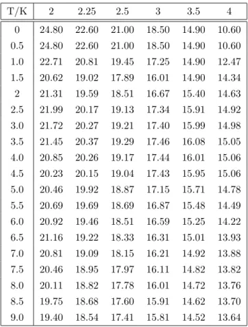
In this section we calibrate the model (17)-(19) to market data available on 14.08.2007. The caplet-strike volatility matrix is partially shown in Table 1.

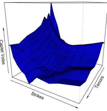
The corresponding implied volatility surface is shown in Figure 1.

Pronounced smiles are clearly observable. Due to the structure of the given data we are going to calibrate the jump diffusion model based on semi-annual tenors, i.e. δ_j ≡ 0.5, with n = 41, and where the initial calibration date 14.08.2007 is identified withT₀= 0.

In a pre-calibration a standard market model is calibrated to ATM caps and ATM swaptions using Schoenmakers (2005). However, we emphasize that the method by which this input market model is obtained is not essential nor a discussion point for this paper. For the pre-calibration we have used a volatility structure of the form

γ_i(t) =c_ig(T_i−t)e_i, 0≤t≤T_i, 1≤i < n,

where g is a simple parametric function and ei are unit vectors. The pre- calibration routine returnsei∈Rⁿ⁻¹ such that (ei,k) is upper triangular and

e^>_i ej =ρij = exp

−|j−i|

m−1(−lnρ_∞

−ηi²+j²+ij−mi−mj−3i−3j+ 3m+ 2 (m−2)(m−3)

, (35) i, j= 1, . . . , m:=n−1, 0≤η≤ −lnρ_∞,

withn= 41, ρ∞= 0.23, η= 1.42.The function gis given by g(s) =g_∞+ (1−g_∞+as)e^−bs.

witha= 0.32, b= 0.07, andg_∞= 0.58. The loading factorsci can be readily computed from

(σ^{AT M}_T_i )²Ti =c²_i Z T_i

0

g²(s)ds, i= 1, . . . , n−1,

(15)

T/K 2 2.25 2.5 3 3.5 4 0 24.80 22.60 21.00 18.50 14.90 10.60 0.5 24.80 22.60 21.00 18.50 14.90 10.60 1.0 22.71 20.81 19.45 17.25 14.90 12.47 1.5 20.62 19.02 17.89 16.01 14.90 14.34 2 21.31 19.59 18.51 16.67 15.40 14.63 2.5 21.99 20.17 19.13 17.34 15.91 14.92 3.0 21.72 20.27 19.21 17.40 15.99 14.98 3.5 21.45 20.37 19.29 17.46 16.08 15.05 4.0 20.85 20.26 19.17 17.44 16.01 15.06 4.5 20.23 20.15 19.04 17.43 15.95 15.06 5.0 20.46 19.92 18.87 17.15 15.71 14.78 5.5 20.69 19.69 18.69 16.87 15.48 14.49 6.0 20.92 19.46 18.51 16.59 15.25 14.22 6.5 21.16 19.22 18.33 16.31 15.01 13.93 7.0 20.81 19.09 18.15 16.21 14.92 13.88 7.5 20.46 18.95 17.97 16.11 14.82 13.82 8.0 20.11 18.82 17.78 16.01 14.72 13.76 8.5 19.75 18.68 17.60 15.91 14.62 13.70 9.0 19.40 18.54 17.41 15.81 14.52 13.64

Table 1: Caplet volatilities σ^K_T(in %) for different strikes and different tenor dates (in years).

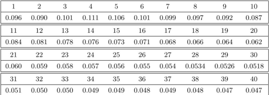
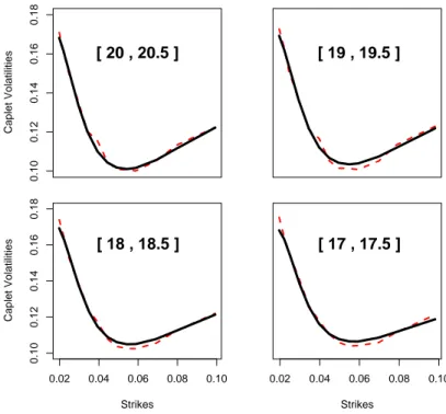
using the initial Libor curve, which is obtained by a standard stripping procedure from the yield curve at 14.08.2007. Table 2 shows the calibrated values of c_i. Finally, the calibration procedure presented in Section 5 delivers the following parameter values: r= 0.18 andρ, σ, κvarying across several chosen maturities as shown in Table 3. The quality of the calibration can be seen in Figure 2, where calibrated volatility curves are shown for several caplet periods (corresponding to Table 7) together with the market caplet volas. The overall relative root- mean-square fit we have reached shows to be 0.5%-5%, when the caplet maturity ranges from 0.5 to 20.

(16)

Tenors Strikes

Caplet Volas

Figure 1: Caplet implied volatility surfaceσ^K_T.

8 Appendix

8.0.1 The Conditional Characteristic Function

We need to determine the conditional characteristic function of lnL_j(T) given Lj(0) for all j= 1, ..., n−1.under the relevant measurePj+1when the Heston CIR-process has for each component k= 1, ..., n−1 the general form

dv_k =κ^(j+1)_k (θ^(j+1)_k −v_k)dt+σ_kρ_k√

v_kdfW_k^(j+1)+σ_k q

(1−ρ²_k)√

v_kdW^(j+1)_k , (36)

(17)

1 2 3 4 5 6 7 8 9 10 0.096 0.090 0.101 0.111 0.106 0.101 0.099 0.097 0.092 0.087

11 12 13 14 15 16 17 18 19 20

0.084 0.081 0.078 0.076 0.073 0.071 0.068 0.066 0.064 0.062

21 22 23 24 25 26 27 28 29 30

0.060 0.059 0.058 0.057 0.056 0.055 0.054 0.0534 0.0526 0.0518

31 32 33 34 35 36 37 38 39 40

0.051 0.050 0.050 0.049 0.049 0.048 0.049 0.048 0.047 0.047

Table 2: The values of loadings factorscicalibrated to ATM caplets volatilities.

Tenor 20 19 18 17

ρ -0.7832 -0.7832 -0.7832 -0.7832 σ 7.4920 7.4920 6.2427 5.0198 κ 2.3376 2.3376 3.9385 4.5590

Table 3: Parameters estimates for chosen tenors.

In this case and a forward Libor dynamic given by (34) , with generalv∈Rⁿ⁻¹, the solution is of the form

ϕj+1(z;T, l, v) =Ej+1

h

e^iz^ln^L^j^(T⁾

Lj(0) =l, vk(0) =vk, k= 1, ..., n−1i

=ϕ_j+1,0(z;T) exp(izlnl)

n−1

Y

k=j

ϕ_j+1,k(z;T) (37)

where

ϕj+1,0(z;T) = exp

−1

2(1−r²)η_j²(T) z²+iz

, η²_j(T) = Z T

0

|γj|²dt

and eachϕ_j+1,k(z;T) =ϕ_j+1,k(z;T, l, v_k) satisfies the parabolic equation

∂ϕj+1,k

∂T =κ^(j+1)_k (θ^(j+1)_k −vk)∂ϕj+1,k

∂v_k −1 2r²γ²_jkvk

∂ϕj+1,k

∂l +1 2σ_k²vk

∂²ϕj+1,k

∂v²_k +1

2r²γ²_jkvk

∂²ϕj+1,k

∂l² +σkρkrγ_jkvk

∂²ϕj+1,k

∂v_k∂l with the terminal condition

ϕj+1,k(z; 0, l, vk) = 1, as can be easily verified by the Feynman-Kac formula.

(18)

0.100.120.140.160.18

Caplet Volatilities

[ 20 , 20.5 ] [ 19 , 19.5 ]

0.02 0.04 0.06 0.08 0.10

0.100.120.140.160.18

Strikes

Caplet Volatilities

[ 18 , 18.5 ]

0.02 0.04 0.06 0.08 0.10 Strikes

[ 17 , 17.5 ]

Figure 2: Caplet volas from the calibrated model (solid lines) and market caplets volasσ^K_T (dashed lines) for different caplet periods.

Sinceγ_j are constant, the above equation can be solved explicitly. The ansatz ϕj+1,k(z;T, l, vk) = exp (Aj,k(z;T) +vkBj,k(z;T))

will yield

A_j,k(z;T) =κ^(j+1)_k θ_k^(j+1) σ_k²

(a_j,k+d_j,k)T−2 ln

1−g_j,ke^d^j,k^T 1−gj,k

Bj,k(z;T) =(aj,k+dj,k)(1−e^d^j,k^T) σ²_k(1−gj,ke^d^j,k^T) , where

aj,k=κ^(j+1)_k −irρkσkγ_jkz dj,k=

q

a²_j,k+r²γ²_jkσ_k²(z²+iz) g_j,k=aj,k+dj,k

a_j,k−d_j,k.

(19)

Note that the first lower index j + 1 at the characteristic function refers to the measure, whereas the first indexj at the introduced coefficients refers to relevant forward Libor. The second index refers to the component.

It is again the choice ofγ that enables the product in (37) to be startet at j.

This crucial feature will show to be beneficial in the calibration part. When j=n−1, for example, only the last ln-Libor will contribute a non-trivial factor to the characteristic function. For all others we have

ϕ_n,k ≡1, k= 1, ..., n−2.

8.0.2 CIR

Consider a CIR model of the form dv(t) =κ(θ−v(t))dt+σp

v(t)dW(t), κ, θ, σ >0.

Givenv(u),v(t) witht > uis distributed with density νχ²_d(νx, ξ)

whereχ²_d(x, ξ) is the density of a noncentral chi-square random variable withd degrees of freedom and noncentrality parameterξand

ν= 4κ

σ²(1−e^−κ(t−u)) ξ= 4κe^−κ(t−u)

σ²(1−e^−κ(t−u))v(u) d= 4θκ

σ² . The conditional mean ofv(t) is given by

E(v(t)|v(u)) =ν⁻¹(ξ+d) = (v(u)−θ)e^−κ(t−u)+θ and the conditional second moment is

E(v²(t)|v(u)) = (2(d+ 2ξ) + (ξ+d)²) ν²

=

1 + 2 d

[E(v(t)|v(u))]²−2

de^{−2κ(t−u)}v²(u).

(20)

8.0.3 Measure Invariance

Why isdW^(n,i+1)_k invariant under the various measures?

See Jamshidian for the compensator, which is given by µⁱ⁺¹

W⁽ⁿ⁾_k =hW⁽ⁿ⁾_k ,lnMi.

with

M = Πⁿ⁻¹_j=i+1(1 +δL_j).

That is, we have

hW⁽ⁿ⁾_k ,lnMi=dW⁽ⁿ⁾_k dlnM =dW⁽ⁿ⁾_k d





n−1

X

j=i+1

ln (1 +δLj)





=

n−1

X

j=i+1

dW⁽ⁿ⁾_k dln(1 +δLj)

=

n−1

X

j=i+1

δLj

1 +δLj

dW⁽ⁿ⁾_k dlnLj

A closer look at (15) reveils that all terms are negligible, since of higher order thandt, or zero due to independence ofW andW or fW, respectively. We thus have

hW⁽ⁿ⁾_k ,lnMi= 0 or in other words, as indicated bydW^(n,i+1)_k :

dW⁽ⁿ⁾_k =dW⁽ⁱ⁺¹⁾_k . Analoguosly we obtain by exchangingWk withWfk that

hfW_k⁽ⁿ⁾,lnMi=dfW_k⁽ⁿ⁾dlnM

=

n−1

X

j=i+1

δLj

1 +δL_jdfW_k⁽ⁿ⁾dlnLj

=

n−1

X

j=i+1

rδLj

1 +δL_jβjk

q v^k_tdt

(21)

References

[1] Andersen, L. and R. Brotherton-Ratcliffe (2001). Extended Libor Market Models with Stochastic Volatility. Working paper, Gen Re Securities.

[2] Andersen, L. and Piterbarg, V. (2007). Moment Explosions in Stochastic Volatility Models.Finance Stoch. 11, no. 1, 29–50.

[3] Belomestny, D. and M. Reiß (2006). Optimal calibration of exponential L´evy models.Finance Stoch. 10, no. 449-474, 29–50.

[4] Belomestny, D. and J.G.M. Schoenmakers (2006).A Jump-Diffusion Libor Model and its Robust Calibration, Preprint No. 1113, WIAS Berlin.

[5] Brigo, D. and F. Mercurio (2001)Interest rate models—theory and practice.

Springer Finance. Springer-Verlag, Berlin.

[6] Brace, A., Gatarek, D. and M. Musiela (1997). The Market Model of Interest Rate Dynamics.Mathematical Finance,7(2), 127–155.

[7] Carr, P. and D. Madan (1999). Option Valuation Using the Fast Fourier Transform,Journal of Computational Finance,2, 6174.

[8] Cox, J.C., Ingersoll, J.E. and S.A. Ross (1985). A Theory of the Term Struc- ture of Interest Rates,Econometrica 53, 385-407.

[9] Eberlein, E., Keller U. and K. Prause (1998). New insights into smile, mis- pricing, and value at risk: the hyperbolic model.Journal of Business,71(3), 371405.

[10] Eberlein, E. and F. ¨Ozkan (2005). The L´evy Libor model, Finance Stoch.

7, no. 1, 1–27.

[11] Glasserman, P.Monte Carlo methods in financial engineering. Applications of Mathematics (New York),53. Stochastic Modelling and Applied Proba- bility. Springer-Verlag, New York, 2004.

[12] Glasserman, P. and S.G. Kou (2003). The term structure of simple forward rates with jump risk.Mathematical Finance 13, no. 3, 383–410.

[13] Heston, S. (1993). A closed-form solution for options with stochastic volatility with applications to bond and currency options.The Review of Financial Studies, Vol. 6, No. 2, 327-343.

[14] Jamshidan, F.(1997). LIBOR and swap market models and measures. Fi- nance and Stochastics,1, 293–330.

[15] Jamshidian, F.(2001). LIBOR Market Model with Semimartingales, in Op- tion Pricing, Interest Rates and Risk Management, Cambridge Univ.

(22)

[16] Kahl Ch. and P. J¨ackel (2006). Fast strong approximation Monte Carlo schemes for stochastic volatility models. Quantitative Finance, 6(6), 513–

536.

[17] Kurbanmuradov, O., Sabelfeld, K. and J. Schoenmakers(2002) Lognormal approximations to Libor market models.Journal of Computational Finance, 6(1), 69–100.

[18] Merton, R.C. (1976). Option pricing when underlying stock returns are discontinuous.J. Financial Economics,3(1), 125–144.

[19] Miltersen, K., K. Sandmann, and D. Sondermann (1997). Closed-form so- lutions for term structure derivatives with lognormal interest rates.Journal of Finance, 409-430.

[20] Piterbarg,V. (2004). A stochastic volatility forward Libor model with a term structure of volatility smiles. Working paper. SSRN.

[21] Schoenmakers, J.: Robust Libor Modelling and Pricing of Derivative Prod- ucts. BocaRaton London NewYork Singapore: Chapman & Hall – CRC Press 2005

[22] Wu, L. and F. Zhang (2006). Libor Market Model with Stochastic Volatility.

Journal of Industrial and Management Optimization, 2, 199–207.

[23] Zhu, J. (2007). An extended Libor Market Model with nested stochastic volatility dynamics. Working paper. SSRN.

(23)

SFB 649 Discussion Paper Series 2007

For a complete list of Discussion Papers published by the SFB 649, please visit http://sfb649.wiwi.hu-berlin.de.

001 "Trade Liberalisation, Process and Product Innovation, and Relative Skill Demand" by Sebastian Braun, January 2007.

002 "Robust Risk Management. Accounting for Nonstationarity and Heavy Tails" by Ying Chen and Vladimir Spokoiny, January 2007.

003 "Explaining Asset Prices with External Habits and Wage Rigidities in a DSGE Model." by Harald Uhlig, January 2007.

004 "Volatility and Causality in Asia Pacific Financial Markets" by Enzo Weber,

January 2007.

005 "Quantile Sieve Estimates For Time Series" by Jürgen Franke, Jean- Pierre Stockis and Joseph Tadjuidje, February 2007.

006 "Real Origins of the Great Depression: Monopolistic Competition, Union Power, and the American Business Cycle in the 1920s" by Monique Ebell and Albrecht Ritschl, February 2007.

007 "Rules, Discretion or Reputation? Monetary Policies and the Efficiency of Financial Markets in Germany, 14th to 16th Centuries" by Oliver Volckart, February 2007.

008 "Sectoral Transformation, Turbulence, and Labour Market Dynamics in Germany" by Ronald Bachmann and Michael C. Burda, February 2007.

009 "Union Wage Compression in a Right-to-Manage Model" by Thorsten Vogel, February 2007.

010 "On σ−additive robust representation of convex risk measures for unbounded financial positions in the presence of uncertainty about the market model" by Volker Krätschmer, March 2007.

011 "Media Coverage and Macroeconomic Information Processing" by Alexandra Niessen, March 2007.

012 "Are Correlations Constant Over Time? Application of the CC-TRIG_t-test to Return Series from Different Asset Classes." by Matthias Fischer, March 2007.

013 "Uncertain Paternity, Mating Market Failure, and the Institution of Marriage" by Dirk Bethmann and Michael Kvasnicka, March 2007.

014 "What Happened to the Transatlantic Capital Market Relations?" by Enzo Weber, March 2007.

015 "Who Leads Financial Markets?" by Enzo Weber, April 2007.

016 "Fiscal Policy Rules in Practice" by Andreas Thams, April 2007.

017 "Empirical Pricing Kernels and Investor Preferences" by Kai Detlefsen, Wolfgang Härdle and Rouslan Moro, April 2007.

018 "Simultaneous Causality in International Trade" by Enzo Weber, April 2007.

019 "Regional and Outward Economic Integration in South-East Asia" by Enzo Weber, April 2007.

020 "Computational Statistics and Data Visualization" by Antony Unwin, Chun-houh Chen and Wolfgang Härdle, April 2007.

021 "Ideology Without Ideologists" by Lydia Mechtenberg, April 2007.

022 "A Generalized ARFIMA Process with Markov-Switching Fractional Differencing Parameter" by Wen-Jen Tsay and Wolfgang Härdle, April 2007.

SFB 649, Spandauer Straße 1, D-10178 Berlin http://sfb649.wiwi.hu-berlin.de

(24)

023 "Time Series Modelling with Semiparametric Factor Dynamics" by Szymon Borak, Wolfgang Härdle, Enno Mammen and Byeong U. Park,

April 2007.

024 "From Animal Baits to Investors’ Preference: Estimating and Demixing of the Weight Function in Semiparametric Models for Biased Samples" by Ya’acov Ritov and Wolfgang Härdle, May 2007.

025 "Statistics of Risk Aversion" by Enzo Giacomini and Wolfgang Härdle,

May 2007.

026 "Robust Optimal Control for a Consumption-Investment Problem" by Alexander Schied, May 2007.

027 "Long Memory Persistence in the Factor of Implied Volatility Dynamics"

by Wolfgang Härdle and Julius Mungo, May 2007.

028 "Macroeconomic Policy in a Heterogeneous Monetary Union" by Oliver Grimm and Stefan Ried, May 2007.

029 "Comparison of Panel Cointegration Tests" by Deniz Dilan Karaman Örsal, May 2007.

030 "Robust Maximization of Consumption with Logarithmic Utility" by Daniel Hernández-Hernández and Alexander Schied, May 2007.

031 "Using Wiki to Build an E-learning System in Statistics in Arabic Language" by Taleb Ahmad, Wolfgang Härdle and Sigbert Klinke, May 2007.

032 "Visualization of Competitive Market Structure by Means of Choice Data"

by Werner Kunz, May 2007.

033 "Does International Outsourcing Depress Union Wages? by Sebastian Braun and Juliane Scheffel, May 2007.

034 "A Note on the Effect of Outsourcing on Union Wages" by Sebastian Braun and Juliane Scheffel, May 2007.

035 "Estimating Probabilities of Default With Support Vector Machines" by Wolfgang Härdle, Rouslan Moro and Dorothea Schäfer, June 2007.

036 "Yxilon – A Client/Server Based Statistical Environment" by Wolfgang Härdle, Sigbert Klinke and Uwe Ziegenhagen, June 2007.

037 "Calibrating CAT Bonds for Mexican Earthquakes" by Wolfgang Härdle and Brenda López Cabrera, June 2007.

038 "Economic Integration and the Foreign Exchange" by Enzo Weber, June 2007.

039 "Tracking Down the Business Cycle: A Dynamic Factor Model For Germany 1820-1913" by Samad Sarferaz and Martin Uebele, June 2007.

040 "Optimal Policy Under Model Uncertainty: A Structural-Bayesian Estimation Approach" by Alexander Kriwoluzky and Christian Stoltenberg, July 2007.

041 "QuantNet – A Database-Driven Online Repository of Scientific Information" by Anton Andriyashin and Wolfgang Härdle, July 2007.

042 "Exchange Rate Uncertainty and Trade Growth - A Comparison of Linear and Nonlinear (Forecasting) Models" by Helmut Herwartz and Henning Weber, July 2007.

043 "How do Rating Agencies Score in Predicting Firm Performance" by Gunter Löffler and Peter N. Posch, August 2007.

(25)

044 "Ein Vergleich des binären Logit-Modells mit künstlichen neuronalen Netzen zur Insolvenzprognose anhand relativer Bilanzkennzahlen" by Ronald Franken, August 2007.

045 "Promotion Tournaments and Individual Performance Pay" by Anja Schöttner and Veikko Thiele, August 2007.

046 "Estimation with the Nested Logit Model: Specifications and Software Particularities" by Nadja Silberhorn, Yasemin Boztuğ and Lutz Hildebrandt, August 2007.

047 "Risiken infolge von Technologie-Outsourcing?" by Michael Stephan, August 2007.

048 "Sensitivities for Bermudan Options by Regression Methods" by Denis Belomestny, Grigori Milstein and John Schoenmakers, August 2007.

049 "Occupational Choice and the Spirit of Capitalism" by Matthias Doepke and Fabrizio Zilibotti, August 2007.

050 "On the Utility of E-Learning in Statistics" by Wolfgang Härdle, Sigbert Klinke and Uwe Ziegenhagen, August 2007.

051 "Mergers & Acquisitions and Innovation Performance in the Telecommunications Equipment Industry" by Tseveen Gantumur and Andreas Stephan, August 2007.

052 "Capturing Common Components in High-Frequency Financial Time Series: A Multivariate Stochastic Multiplicative Error Model" by Nikolaus Hautsch, September 2007.

053 "World War II, Missing Men, and Out-of-wedlock Childbearing" by Michael Kvasnicka and Dirk Bethmann, September 2007.

054 "The Drivers and Implications of Business Divestiture – An Application and Extension of Prior Findings" by Carolin Decker, September 2007.

055 "Why Managers Hold Shares of Their Firms: An Empirical Analysis" by Ulf von Lilienfeld-Toal and Stefan Ruenzi, September 2007.

056 "Auswirkungen der IFRS-Umstellung auf die Risikoprämie von Unternehmensanleihen - Eine empirische Studie für Deutschland, Österreich und die Schweiz" by Kerstin Kiefer and Philipp Schorn,

September 2007.

057 "Conditional Complexity of Compression for Authorship Attribution" by Mikhail B. Malyutov, Chammi I. Wickramasinghe and Sufeng Li,

September 2007.

058 "Total Work, Gender and Social Norms" by Michael Burda, Daniel S.

Hamermesh and Philippe Weil, September 2007.

059 "Long-Term Orientation in Family and Non-Family Firms: a Bayesian Analysis" by Jörn Hendrich Block and Andreas Thams, October 2007 060 "Kombinierte Liquiditäts- und Solvenzkennzahlen und ein darauf basierendes Insolvenzprognosemodell für deutsche GmbHs" by

Volodymyr Perederiy, October 2007

061 "Embedding R in the Mediawiki" by Sigbert Klinke and Olga Zlatkin- Troitschanskaia, October 2007

062 "Das Hybride Wahlmodell und seine Anwendung im Marketing" by Till Dannewald, Henning Kreis and Nadja Silberhorn, November 2007

063 "Determinants of the Acquisition of Smaller Firms by Larger Incumbents in High-Tech Industries: Are they related to Innovation and Technology Sourcing? " by Marcus Wagner, November 2007

(26)

064 "Correlation vs. Causality in Stock Market Comovement" by Enzo Weber, October 2007

065 "Integrating latent variables in discrete choice models – How higher- order values and attitudes determine consumer choice" by Dirk Temme, Marcel Paulssen and Till Dannewald, December 2007

066 "Modelling Financial High Frequency Data Using Point Processes" by Luc Bauwens and Nikolaus Hautsch, November 2007

067 "A stochastic volatility Libor model and its robustcalibration" by Denis Belomestny, Stanley Matthew and John Schoenmakers, December 2007