• Keine Ergebnisse gefunden

Worksheet 10: Integration June 6, 2014

N/A
N/A
Protected

Academic year: 2021

Aktie "Worksheet 10: Integration June 6, 2014"

Copied!
2
0
0

Wird geladen.... (Jetzt Volltext ansehen)

Volltext

(1)

Physik auf dem Computer SS 2014

Worksheet 10: Integration

June 6, 2014

General Remarks

• The deadline for the worksheets is Wednesday, 25 June 2014, 10:00 for the tutorial on Friday and Friday, 27 June 2014, 10:00 for the tutorials on Tuesday and Wednesday.

• On this worksheet, you can achieve a maximum of 10 points.

• To hand in your solutions, send an email to

Johannes ( zeman@icp.uni-stuttgart.de ; Tuesday, 9:45–11:15) Tobias (richter@icp.uni-stuttgart.de; Wednesday, 15:45–17:15) Shervin ( shervin@icp.uni-stuttgart.de ; Friday, 11:30–13:00) Task 10.1: One-dimensional Integration (7 points)

The error function is a sigmoidal function that is used in statistics and some other areas. It is defined as

erf(x) = 2

π

x

Z

0

e −τ

2

dτ (1)

The job in this task is to implement the error function.

10.1.1 (1 point) Implement a Python function integrate1d_midpoint(f,a,b,N) that approxi- mates R a b f(x) dx using the midpoint rule with N support points.

10.1.2 (1 point) Implement a Python function integrate1d_romberg(f,a,b,N) that approx- imates R a b f(x) dx using Romberg’s method with N support points on the finest level, i. e. use h = N b−a −1 as smallest step size.

Hint Note that the implementation in the lecture script uses N = 2 kmax support points, so choose kmax accordingly.

10.1.3 (1 point) Implement a Python function integrate1d_mc(f,a,b,N) that approximates R b

a f(x) dx using N steps of Monte-Carlo Integration.

10.1.4 (1 point) Implement the Python functions erf_midpoint(x,N) ,

erf_romberg(x,N) and erf_mc(x,N) that compute the error function for N points with the cor- responding integration rules.

10.1.5 (1 point) Evaluate the error function erf(x) on the interval [0, 2.0] at 100 equidistant points x using erf_romberg with N = 64, and plot the resulting approximation of the error function.

10.1.6 (1 point) Compute a reference value e ref = erf(1) using Romberg’s method with N = 512. Create a loglog plot of the accuracy of all implemented methods when computing erf(1) for N ∈ {4, 8, 16, 32, 64, 128, 256, 512}.

1

(2)

10.1.7 (1 point) Use the integrate1d_* functions to approximate π via π

4 = Z 1

0

p 1 − x 2 dx (2)

Create a loglog plot of the accuracy of the different integration schemes versus the number of points N ∈ {4, 8, 16, . . . , 512}. Use numpy.pi as reference value. Why does the accuracy behave differently this time?

Task 10.2: Multidimensional Monte-Carlo Integration (3 points)

In Gaussian units ( = 1), the interaction energy of two homogenously charged bodies V 1 and V 2 is given by

E = Z

V

1

Z

V

2

1

|~ x 1~ x 2 | d~ x 1 d~ x 2

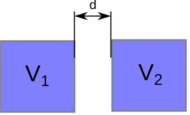
In this task, we consider the interaction of two homogenously charged cubes (in 3D; Q = 1) V 1 and V 2 with side length 1 at a distance d (see the figure below).

Figure 1: Two homogenously charged cubes V 1 and V 2 at distance d.

10.2.1 (2 points) Write a Python function that computes the interaction energy of the cubes at distance d using Monte-Carlo integration with N = 1000 steps.

10.2.2 (1 point) Compute the interaction energy for 10 different values of d between 10 −2 and 10 2 . Plot the interaction energy E versus the distance d in log-log-scale. In the same figure, add a plot of the interaction energy of two unit point charges at distance d.

2

Abbildung

Figure 1: Two homogenously charged cubes V 1 and V 2 at distance d.

Referenzen

ÄHNLICHE DOKUMENTE

В ближайшие годы также не прогнозируется существенного роста инновационной активно- сти промышленных организаций, особенно низким уровнем

In fact, we shall see that our problem is equivalent to determining the maximum number of translated copies of a regular n-dimensional simplex that can be placed in R n such that

I want to introduce to you the idea of interconnecting the subject-specific online reference service EconDesk 1 of the German National Library of Economics (ZBW) with the

The pentagrams denote poly-T Stretch, and the location and copy number of other repeat types are shown by colored dots: orange represents the second type; purple represents the

Based on an extended technology acceptance model (TAM), we therefore analyzed the moderating effects of Hofstede’s cultural dimensions on technological, social, and

Official import ban for MBM and ruminants from GB Elimination of risk material from animals > 6 month 1988: → No more import licences given for MBM from GB.. 1993: → MBM

Session 1 set the scene for the seminar by discussing the economic backdrop that would underpin discussions at the Leaders’ Summit in Brisbane. It was suggested that the

During this analysis we classified tests into unit and integration tests according to the definitions of the Institute of Electrical and Electronics Engineers (IEEE) and