table isotope geochemistry is concerned with variations of the isotopic compositions of elements arising from physicochemical processes rather than nuclear processes. Fractionation

W . M . W h i t e G e o c h e m i s t r y Chapter 9: Stable Isotopes

Chapter 9: Stable Isotope Geochemistry

9.1 Introduction

table isotope geochemistry is concerned with variations of the isotopic compositions of elements arising from physicochemical processes rather than nuclear processes. Fractionation

of the iso- topes of an element might at first seem to be an oxymoron. After all, in the last chapter we saw that the value of radiogenic isotopes was that the various isotopes of an element had identical chemical properties and therefore that isotope ratios such as

Sr/

Sr are not changed measurably by chemical processes. In this chapter we will find that this is not quite true, and that the very small differences in the chemical behavior of different isotopes of an element can provide a very large amount of useful in- formation about chemical (both geochemical and biochemical) processes.

The origins of stable isotope geochemistry are closely tied to the development of modern physics in the first half of the 20

century. The discovery of the neutron in 1932 by H. Urey and the demonstration of variations in the isotopic composition of light elements by A. Nier in the 1930’s and 1940’s were the precursors to the development of stable isotope geochemistry. The real history of stable isotope geo- chemistry begins in 1947 with the Harold Urey’s publication of a paper entitled “The Thermodynamic Properties of Isotopic Substances”. Urey not only showed why, on theoretical grounds, isotope fraction- ations could be expected, but also suggested that these fractionations could provide useful geological information. Urey then set up a laboratory to determine the isotopic compositions of natural sub- stances and experimentally determine the temperature dependence of isotopic fractionations, in the process establishing the field of stable isotope geochemistry.

What has been learned in the fifty years since that paper was published would undoubtedly as- tonish even Urey. Stable isotope geochemistry, like radiogenic isotope geochemistry, has become an essential part of not only geochemistry, but the earth sciences as a whole. In this chapter, we will at- tempt to gain an understanding of the principles underlying stable isotope geochemistry and then briefly survey its many-fold applications in the earth sciences. In doing so, we add the final tool to our geochemical toolbox.

9.1.1 Scope of Stable Isotope Geochemistry

The principal elements of interest in stable isotope geochemistry are H, Li, B, C, N, O, Si, S, and Cl.

Of these, O, H, C and S are of the greatest interest. Most of these elements have several common char- acteristics:

(1) They have low atomic mass.

(2) The relative mass difference between their isotopes is large.

(3) They form bonds with a high degree of covalent character.

(4) The elements exist in more than one oxidation state (C, N, and S), form a wide variety of com- pounds (O), or are important constituents of naturally occurring solids and fluids.

(5) The abundance of the rare isotope is sufficiently high (generally at least tenths of a percent) to fa- cilitate analysis.

It was once thought that elements not meeting these criteria would not show measurable variation in isotopic composition. However, as new techniques offering greater sensitivity and higher precision have become available (particularly use of the MC-ICP-MS), geochemists have begun to explore iso- topic variations of metals such as Mg, Ca, Ti, Cr, Fe, Zn, Cu, Ge, Se, Mo, and Tl. The isotopic variations observed in these metals have generally been quite small. Nevertheless, some geologically useful in- formation has been obtained from isotopic study of these metals and exploration of their isotope geo- chemistry continues. We do not have space to consider them here, but their application is reviewed in a recent book (Johnson et al., 2004).

The elements of interest in radiogenic isotope geochemistry are heavy (Sr, Nd, Hf, Os, Pb), most form dominantly ionic bonds, generally exist in only one oxidation state, and there is only small rela-

*

Fractionation refers to the change in an isotope ratio that arises as a result of some chemical or physical process.

S

W . M . W h i t e G e o c h e m i s t r y Chapter 9: Stable Isotopes

tive mass differences be- tween the isotopes of inter- est. Thus isotopic fractiona- tion of these elements is quite small and can gen- erally be ignored. Further- more, any natural frac- tionation is corrected for in the process of correcting much larger fractionations that typically occur during analysis (with the exception of Pb). Thus is it that one group of isotope geochemists make their living by measuring isotope frac- tionations while the other group makes their living by ignoring them!

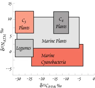
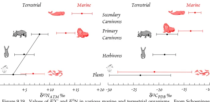
Stable isotope geochemistry has been be applied to a great variety of problems, and we will see a number of examples in this chapter. One of the most common is geothermometry. Another is process identification. For instance, plants that produce ‘C

’ hydrocarbon chains (that is, hydrocarbon chains 4 carbons long) as their primary photosynthetic product fractionate carbon differently than to plants that produce ‘C

’ chains. This fractionation is retained up the food chain. This allows us, for example, to draw some inferences about the diet of fossil mammals from the stable isotope ratios in their bones.

Sometimes stable isotope ratios are used as 'tracers' much as radiogenic isotopes are. So, for example, we can use oxygen isotope ratios in igneous rocks to determine whether they have assimilated crustal material, as crust generally has different O isotope ratios than does the mantle.

9.1.2 Some Definitions 9.1.2.1The δ Notation

As we shall see, variations in stable isotope ratios are typically in the parts per thousand to parts per hundred range and are most conveniently and commonly reported as permil deviations, δ, from some standard. For example, O isotope ratios are often reported as permil deviations from SMOW (standard mean ocean water) as:

!

O = (

O /

O)

" (

O /

O)

(

O /

O)

#

$ % &

' ( ) 10

9.1

Unfortunately, a dual standard developed for reporting O isotopes. While O isotopes in most sub- stances are reported relative to SMOW, the oxygen isotope composition of carbonates is reported rela- tive to the Pee Dee Belemite (PDB) carbonate standard

. This value is related to SMOW by:

δ

O

= 1.03086δ

O

+ 30.86 9.2

A similar δ notation is used to report other stable isotope ratios. Hydrogen isotope ratios, δD, are also reported relative to SMOW, carbon isotope ratios relative to PDB, nitrogen isotope ratios relative to atmospheric nitrogen (denoted ATM), and sulfur isotope ratios relative to troilite in the Canyon Diablo iron meteorite (denoted CDT). Table 9.1 lists the isotopic composition of these standards.

9.1.2.2 The Fractionation Factor

The fractionation factor, α, is the ratio of isotope ratios in two phases:

!

# R

R

^9.3

‡

There is, however, a good historical reason for this: analytical difficulties in the measurement of carbonate oxygen prior to 1965 required it be measured against a carbonate standard.

Table 9.1. Isotope Ratios of Stable Isotopes

Element Notation Ratio Standard Absolute Ratio Hydrogen δD D/H (

H/

H) SMOW 1.557 × 10

Lithium δ

Li

Li/

Li NIST 8545 (L-SVEC) 12.285

Boron δ

B

B/

B NIST 951 4.044

Carbon δ

C

C/

C PDB 1.122 × 10

Nitrogen δ

N

N/

N atmosphere 3.613 × 10

Oxygen δ

O

O/

O SMOW, PDB 2.0052 × 10

δ

O

O/

O SMOW 3.76 × 10

Sulfur δ

S

S/

S CDT 4.43 × 10

W . M . W h i t e G e o c h e m i s t r y Chapter 9: Stable Isotopes

The fractionation of isotopes between two phases is also often reported as ∆

= δ

– δ

. The relation- ship between ∆ and α is:

∆ ≈ (α - 1)10

or ∆ ≈ 10

ln α 9.4

As we will see, at equilibrium, α may be related to the equilibrium constant of thermodynamics by

α A-B = ( K/K

)

9.5

where n is the number of atoms exchanged, K _∞ is the equilibrium constant at infinite temperature, and K is the equilibrium constant written in the usual way (except that concentrations are used rather than activities because the ratios of the activity coefficients are equal to 1, i.e., there are no isotopic effects on the activity coefficient).

9.2 Theoretical Considerations

Isotope fractionation can originate from both kinetic effects and equilibrium effects. The former may be intuitively expected, but the latter may at first seem somewhat surprising. After all, we have been taught that the chemical properties of an element are dictated by its electronic structure, and that the nucleus plays no real role in chemical interactions. In the following sections, we will see that quantum mechanics predicts that the mass of an atom affect its vibrational motion therefore the strength of chemical bonds. It also affects rotational and translational motions. From an understanding of these ef- fects of atomic mass, it is possible to predict the small differences in the chemical properties of isotopes quite accurately.

9.2.1 Equilibrium Isotope Fractionations

Most isotope fractionations arise from equilibrium effects. Equilibrium fractionations arise from transla- tional, rotational and vibrational motions of molecules in gases and liquids and atoms in crystals because the en- ergies associated with these motions are mass dependent. Systems tend to adjust themselves so as to mini- mize energy. Thus isotopes will be distributed so as to minimize the vibrational, rotational, and trans- lational energy of a system. Of the three types of energies, vibrational energy makes by far the most important contribution to isotopic fractionation. Vibrational motion is the only mode of motion avail- able to atoms in a solid. These effects are, as one might expect, small. For example, the equilibrium constant for the reaction

¹ ₂ C

O

+ H

18

O ® ¹ ₂ C

O

+ H

16

O 9.6

is only about 1.04 at 25°C and the ∆G of the reaction, given by –RTln K, is only -100 J/mol (you'll recall most ∆G's for reactions are in typically in the kJ/mol range).

9.2.1.1 The Quantum Mechanical Origin of Isotopic Fractionations

It is fairly easy to understand, at a qualitative level at least, how some isotope fractionations can arise from vibrational motion. Consider the two hydrogen atoms of a hydrogen molecule: they do not remain at a fixed distance from one and other, rather they continually oscillate toward and away from each other, even at absolute zero. The frequency of this oscillation is quantized, that is, only discrete

†

To derive this, we rearrange equation 8.1 to obtain: R

= (δ

+ 10

)R

/ 10

Note that ∆ is sometimes defined as ∆ ≡ 10

ln α, in which case ∆

≈ δ

– δ

.

So that α may be expressed as: α = ^{( !}

^{+ 10}

3

) R

STD

/ 10

(!

+ 10

)R

/ 10

$ ( !

+ 10

)

(!

+ 10

) Subtracting 1 from each side and rearranging, we obtain:

α − 1 = ! " 1 = (#

#

)

(#

+ 10

) & (#

#

)

10

& !' 10

since δ is small. The second equation in 9.4 results from the approximation that for x ≈ 1, ln x ≈ x-1.

W . M . W h i t e G e o c h e m i s t r y Chapter 9: Stable Isotopes

frequency values are possible.

Figure 9.1 is a schematic dia- gram of energy as a function of interatomic distance in the hydrogen molecule. As the atoms vibrate back and forth, their potential energy varies as shown by the curved line.

The zero point energy (ZPE) is the energy level at which the molecule will vibrate in its ground state, which is the state in which the molecule will be in at low temperature.

The zero point energy is al- ways some finite amount above the minimum potential energy of an analogous har- monic oscillator.

The potential energy curves for various isotopic combina- tions of an element are identi- cal, but as the figure shows, the zero point vibrational en- ergies differ, as do vibration energies at higher quantum levels, being lower for the heavier isotopes. Vibration energies and frequencies are directly related to bond strength. Because of this, the energy required for the molecule to dissociate will differ for different isotopic combinations. For exam- ple, 440.6 kJ/mole is necessary to dissociate a D

(

H

) molecule, but only 431.8 kJ/mole is required to dissociate the

H

molecule. Thus the bond formed by the two deuterium atoms is 9.8 kJ/mole stronger than the H–H bond. The differences in bond strength can also lead to kinetic fractionations, since mole- cules that dissociate easier will react faster. We will discuss kinetic fractionations a bit later.

9.2.1.2 Predicting Isotopic Fractionations from Statistical Mechanics

Now let's attempt to understand the origin of isotopic fractionations on a more quantitative level.

We have already been introduced to several forms of the Boltzmann distribution law (e.g., equation 2.84), which describes the distribution of energy states. It states that the probability of a molecule having in- ternal energy E

is:

P

= g

e

g

e

"

^9.7

where g is a statistical weight factor

, k is Boltzmann's constant, and the sum in the denominator is taken over all possible states. The average energy (per molecule) is:

‡

This factor comes into play where more than one state corresponds to an energy level Ei (the states are said to be

‘degenerate’). In that case g

is equal to the number of states having energy level E

.

Figure 9.1. Energy-level diagram for the hydrogen molecule. Funda-

mental vibration frequencies are 4405 cm

for H ₂ , 3817 cm

for HD,

and 3119 cm

for D

. The zero-point energy of H

is greater than that of

HD which is greater than that of D

. Arrows show the energy, in

kJ/mol, required to dissociate the 3 species. After O’Niel (1986).

W . M . W h i t e G e o c h e m i s t r y Chapter 9: Stable Isotopes

E = E

P

!

^{= g}

^E

^e

"Ei/kT

!

g

e

!

^9.8

As we saw in Chapter 2, the partition function, Q, is the denomi- nator of this equation:

Q = g

e

"

^9.9

The partition function is related to thermodynamic quantities U and S (equations 2.90 and 2.91). Since there is no volume change associated with isotope exchange reactions, we can use the rela- tionship:

∆G = ∆U – T∆S 9.10

and equations 2.119 and 2.123 to derive:

!G

= "RT ln Q

$

^9.11

and comparing to equation 3.86, that the equilibrium constant is related to the partition function as:

K = Q

"

^9.12

for isotope exchange reactions. In the exchange reaction above (9.6) this is simply:

K = Q

0.5

Q

216O

Q

Q

218O

9.13

The usefulness of the partition function is that it can be calculated

from quantum mechanics, and from it we can calculate equilibrium fractionations of isotopes.

There are three modes of motion available to gaseous molecules: vibrational, rotational, and transla- tional (Figure 9.2). The partition function can be written as the product of the translational, rotational, vibrational, and electronic partition functions:

Q

= Q

Q

Q

Q

9.14

The electronic configurations and energies of atoms are unaffected by the isotopic differences, so the last term can be ignored in the present context.

The vibrational motion is the most important contributor to isotopic fractionations, and it is the only mode of motion available to atoms in solids. So we begin by calculating the vibrational partition func- tion. We can approximate the vibration of atoms in a simple diatomic molecule such as CO or O

by that of a harmonic oscillator. The energy of a ‘quantum’ oscillator is:

E

= (n + 1 2)h!

9.15

where ν

is the ground state vibrational frequency, h is Plank’s constant and n is the vibrational quan- tum number. The partition function for vibrational motion of a diatomic molecule is given by:

Q

= e

1 ! e

^9.16

‡

‡

Polyatomic molecules have many modes of vibrational motion available to them. The partition function is calcu- lated by summing the energy over all available modes of motion; since energy occurs in the exponent, the result is a product:

Figure 9.2. The three modes of motion, illustrated for a diatom- ic molecule. Rotations can occur about both the y and x axes;

only the rotation about the y

axis is illustrated. Since radial

symmetry exists about the z

axis, rotations about that axis

are not possible according to

quantum mechanics. Three

modes of translational motion

are possible: in the x, y, and z

directions. Possible vibrational

and rotational modes of motion

of polyatomic molecules are

more complex.

W . M . W h i t e G e o c h e m i s t r y Chapter 9: Stable Isotopes

Vibrations of atoms in molecules and crystals approximates that of harmonic oscillators. For an ideal harmonic oscillator, the relation between frequency and reduced mass is:

! = 1

2 k

µ ^9.17

where k is the forcing constant, which depends on the electronic configuration of the molecule, but not the isotope involved, and µ is reduced mass:

µ = 1

1 / m

+ 1 / m

= m

m

m

+ m

^9.18

Hence we see that the vibrational frequency, and therefore also vibrational energy and partition func- tion, depends on the mass of the atoms involved in the bond.

Rotational motion of molecules is also quantized. We can approximate a diatomic molecule as a dumbbell rotating about the center of mass. The rotational energy for a quantum rigid rotator is:

E

= j( j + 1)h

8!

I ^9.19

where j is the rotational quantum number and I is the moment of inertia, I = µr

, where r is the intera- tomic distance. The statistical weight factor, g, in this case is equal to (2j + 1) since there 2 axes about which rotations are possible. For example, if j = 1, then there are j(j + 1) = 2 quanta available to the molecule, and (2j + 1) ways of distributing these two quanta: all to the x-axis, all to the y-axis or one to each. Thus:

Q

= # (2 j + 1)e

^9.20

Because the rotational energy spacings are small, equation 9.20 can be integrated to yield:

Q

= 8!

IkT

" h

^9.21*

where σ is a symmetry factor whose value is 1 for heteronuclear molecules such as

O-

O and 2 for homonuclear molecules such as

O-

O. This arises because in homonuclear molecules, the quanta must be equally distributed between the rotational axes, i.e., the j’s must be all even or all odd. This re- striction does not apply to hetergeneous molecules, hence the symmetry factor.

Finally, translational energy associated with each of the three possible translational motions (x, y, and z) is given by the solution to the Schrödinger equation for a particle in a box:

E

= n

h

8ma

^9.22

where n is the translational quantum number, m is mass, and a is the dimension of the box. This ex- pression can be inserted into equation 9.8. Above about 2 K, spacings between translational energies levels are small, so equ. 9.8 can also be integrated. Recalling that there are 3 degrees of freedom, the re- sult is:

Q

= e

1 ! e

i

" ^9.16a

*

Equation 9.21 also holds for linear polyatomic molecules such as CO

. The symmetry factor is 1 if it has plane sym- metry, and 2 if it does not. For non-linear polyatomic molecules, 9.21 is replaced by:

Q

= 8!

(8!

ABC )

(kT )

"h

9.21a

where A, B, and C are the three principle moments of inertia.

W . M . W h i t e G e o c h e m i s t r y Chapter 9: Stable Isotopes

Q

= (2! mkT )

h

V 9.23

where V is the volume of the box (a

). Thus the full partition function is:

Q

= Q

Q

Q

= e

1 ! e

8"

IkT

# h

(2" mkT )

h

V 9.24

It is the ratio of partition functions that occurs in the equilibrium constant expression, so that many of the terms in 9.24 eventually cancel. Thus the partition function ratio for 2 different isotopic species of the same diatomic molecule, A and B, reduces to:

Q

Q

=

e

1 ! e

I

"

m

e

1 ! e

I

"

m

= e

(1 ! e

)I

"

m

e

(1 ! e

)I

"

m

9.25

Since bond lengths are essentially independent of the isotopic composition, this further reduces to:

Q

Q

= e

(1 ! e

) µ

"

m

e

(1 ! e

) µ

"

m

= e

(1 ! e

) µ

"

m

(1 ! e

) µ

"

m

9.26

Notice that all the temperature terms cancel except for those in the vibrational contribution. Thus vi- brational motion alone is responsible for the temperature dependency of isotopic fractionations.

To calculate the fractionation factor α from the equilibrium constant, we need to calculate K _∞ . For a reaction such as:

aA

+ bB

® aA

+ bB

where A

and A

are two molecules of the same substance differing only in their isotopic composition, and a and b are the stoichiometric coefficients, the equilibrium constant is:

K

= ("

/ "

)

("

/ "

)

^9.27

Thus for a reaction where only a single isotope is exchanged, K _∞ is simply the ratio of the symmetry factors.

9.2.1.3 Temperature Dependence of the Fractionation Factor

As we noted above, the temperature dependence of the fractionation factor depends only on the vi- brational contribution. At temperatures where T<< hν/k, the 1 - e

terms in 9.16 and 9.26 tend to 1 and can therefore be neglected, so the vibrational partition function becomes:

Q

! e

9.28

In a further simplification, since ∆ν is small, we can use the approximation e ^x ≈ 1 + x (valid for x<<1), so that the ratio of vibrational energy partition functions becomes

Q

/ Q

! 1 " h# $ / 2kT

Since the translational and rotational contributions are temperature independent, we expect a relation- ship of the form:

! " A + B

T 9.29

In other words, α should vary inversely with temperature at low temperature.

At higher temperature, the 1 - exp(-h ν /kT) term differs significantly from 1. Furthermore, at higher

vibrational frequencies, the harmonic oscillator approximation breaks down (as suggested in Figure

W . M . W h i t e G e o c h e m i s t r y Chapter 9: Stable Isotopes

9.1), as do several of the other simplifying assumptions we have made, so that the relation between the fractionation factor and temperature approximates:

ln ! " 1

T

9.30

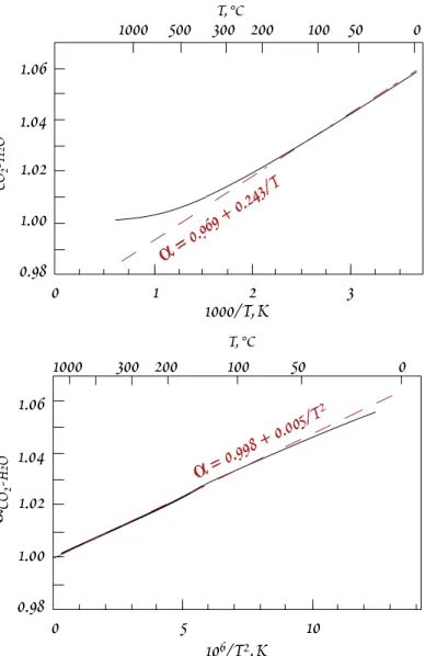
Since α is generally small, ln α ≈ 1 + α, so that α ∝ 1 + 1/T

. At infinite tempera- ture, the fractionation is unity, since ln α

= 0. This illustrated in Figure 9.3 for dis- tribution of

O and

O between CO

and H

O. The α ∝ 1/T relationship breaks down around 200°C; above that tempera- ture the relationship follows α ∝ 1/T

.

It must be emphasized that the simple calculations performed in Example 9.1 are applicable only to a gas whose vibrations can be approximated by a simple har- monic oscillator. Real gases often show fractionations that are complex functions of temperature, with minima, maxima, in- flections, and crossovers. Vibrational modes of silicates, on the other hand, are relatively well behaved.

9.2.1.4 Composition and Pressure Dependence

The nature of the chemical bonds in the phases involved is most important in determining isotopic fractionations. A general rule of thumb is that the heavy isotope goes into the phase in which it is most strongly bound. Bonds to ions with a high ionic potential and low atomic mass are associated with high vibrational frequen- cies and have a tendency to incorporate the heavy isotope preferentially. For ex- ample, quartz, SiO

is typically the most

18

O rich mineral and magnetite the least. Oxygen is dominantly covalently bonded in quartz, but dominantly ionically bonded in magnetite. The O is bound more strongly in quartz than in magnetite, so the former is typically enriched in

O.

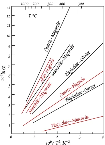
Substitution of cations in a dominantly ionic site (typically the octahedral sites) in silicates has only a secondary effect on the O bonding, so that isotopic fractionations of O isotopes between similar silicates are generally small. Substitutions of cations in sites that have a strong covalent character (generally tet- rahedral sites) result in greater O isotope fractionations. Thus, for example, we would expect the frac- tionation between the end-members of the alkali feldspar series and water to be similar, since only the substitution of K ⁺ for Na ⁺ is involved. We would expect the fractionation factors between end- members of the plagioclase series and water to be greater, since this series involves the substitution of Al for Si as well as Ca for Na, and the bonding of O to Si and Al in tetrahedral sites has a large covalent component.

Figure 9.3. Calculated value of α

O for CO

–H

O, shown vs. 1/T and 1/T

. Dashed lines show that up to ~200° C, α

≈ 0.969 + 0.0243/T. At higher temperatures, α ≈ 0.9983 +

0.0049/T

. Calculated from the data of Richet et al. (1977).

W . M . W h i t e G e o c h e m i s t r y Chapter 9: Stable Isotopes

366 November 30, 2005

Example
 9.1.
 Predicting
 Isotopic
 Fractionations


Consider the exchange of

O and

O between carbon monoxide and oxygen:

C

O +

O

O ® C

O +

O

The frequency for the C-

O vibration is 6.505 × 10

sec

, and the fre quency of the

O

vibration is 4.738 × 10

sec

. How will the fractionation factor, = (

O/

O) _CO /

O/

O) _O

, vary as a function of temperature?

Answer: The equilibrium constant for this reaction is: K = Q

Q

Q

Q

9 . 3 1

The rotational and translational contributions are independent of temperature, so we calculate them first. The rotational contribution is:

K

= Q

Q

Q

Q

⎛

⎝ ⎜ ⎞

⎠ ⎟

rot

= µ

σ

µ

σ

µ

σ

µ

σ

= 1 2

µ

µ

µ

µ

9 . 3 2

(the symmetry factor, , is 2 for

O

and 1 for the other molecules). Substituting values µ _C

_O = 6.857, µ _C

_O = 7.20, µ

_O

_O = 8.471, µ

_O

= 8, we find: K

= 0.9917/2.

The translational contribution is: K

= m

m

m

m

3/ 2

9.33

Substituting m _C

O = 28, m _C

O = 30, m

O

O = 34, m

O

= 32 into 9.33, we find K

= 1.0126.

The vibrational contribution to the equilibrium constant is:

K

= e

(1 − e

)(1 − e

) (1 − e

)(1 − e

)

9 . 3 4

To obtain the v ibrational contribution, we can a ssume the atoms vibrate as harmonic oscillators and, using experimentally determined vibrational frequencies for the

O molecules, solve equation 9.17 for the forcing constant, k, and calculate the vibrational frequencies for the

O-bearing molecules. These turn out to be 6.348 × 10

sec

for C-

O and 4.605 × 10

sec

for

O

O, so that 8.33a becomes:

K

= e

(1 − e

)(1 − e

) (1 − e

)(1 − e

)

If we carry the calculation out at T = 300 K, we find:

K = K

K

K

=

1

2 0.9917 × 1.0126 × 1.1087 = 1.0229 2

To calculate the fr actionation factor from the equilibrium constant, we ne ed to calcu- late K _∞

K

= (1 / 1)

(2 / 1)

= 1

2

so that α = K / K

= 2K

At 300 K, = 1.0233. The variat ion of with temperature is shown in Figure 9.4.

Figure 9.4. Fractionation factor, = (

O/

O) _CO /

(

O/

O) _O

, calculated from partition functions as

a function of temperature.

W . M . W h i t e G e o c h e m i s t r y Chapter 9: Stable Isotopes

367 November 30, 2005

Carbonates tend to be very

O rich because O is bonded to a small, highly charged atom, C

. The fractionation, ∆

O

, between calcite and water is about 30 per mil at 25° C. The cation in the car- bonate has a secondary role (due to the effect of the mass of the cation on vibrational frequency). The

∆

O _carb-H

_O decreases to about 25 when Ba replaces Ca (Ba has about 3 times the mass of Ca).

Crystal structure plays a secondary role. The ∆

O between aragonite and calcite is of the order of 0.5 permil. However, is there apparently a large fractionation (10 permil) of C between graphite and diamond.

Pressure effects on fractionation factors turn out to be small, no more than 0.1 permil over 0.2 GPa.

We can understand the reason for this by recalling that ∂∆G/∂P = ∆V. The volume of an atom is en- tirely determined by its electronic structure, which does not depend on the mass of the nucleus. Thus the volume change of an isotope exchange reaction will be small, and hence there will be little pressure dependence. There will be a minor effect because vibrational frequency and bond length change as crystals are compressed. The compressibility of silicates is of the order of 1 part in 10

, so we can expect effects on the order of 10

or less, which are generally insignificant.

9.2.2 Kinetic Isotope Fractionations

Kinetic isotope fractionations are normally associated with fast, incomplete, or unidirectional proc- esses like evaporation, diffusion, dissociation reactions, and biologically mediated reactions. As an ex- ample, recall that temperature is related to the average kinetic energy. In an ideal gas, the average ki- netic energy of all molecules is the same. The kinetic energy is given by:

E = 1

2 mv

9.35

Consider two molecules of carbon dioxide,

C

O

and

C

O

, in such a gas. If their energies are equal, the ratio of their velocities is (45/44)

, or 1.011. Thus

C

O

can diffuse 1.1% further in a given amount of time than

C

O

. This result, however, is largely limited to ideal gases, i.e., low pressures where collisions between molecules are infrequent and intermolecular forces negligible. For the case where molecular collisions are important, the ratio of their diffusion coefficients is the ratio of the square roots of the reduced masses of CO

and air (mean molecular weight 28.8):

D

D

= µ

µ

= 17.561

17.406 = 1.0044 9.36

Hence we would predict that gaseous diffusion will lead to a 4.4‰ rather than 11‰ fractionation.

Molecules containing the heavy isotope are more stable and have higher dissociation energies than those containing the light isotope. This can be readily seen in Figure 9.1. The energy required to raise the D

molecule to the energy where the atoms dissociate is 441.6 kJ/mole, whereas the energy required to dissociate the H

molecule is 431.8 kJ/mole. Therefore it is easier to break the H-H than D-D bond.

Where reactions attain equilibrium, isotopic fractionations will be governed by the considerations of equilibrium discussed above. Where reactions do not achieve equilibrium the lighter isotope will usually be preferentially concentrated in the reaction products, because of this effect of the bonds involving light iso- topes in the reactants being more easily broken. Large kinetic effects are associated with biologically mediated reactions (e.g., photosynthesis, bacterial reduction), because such reactions generally do not achieve equilibrium and do not go to completion (e.g., plants don’t convert all CO

to organic carbon).

Thus

C is enriched in the products of photosynthesis in plants (hydrocarbons) relative to atmospheric CO

, and

S is enriched in H

S produced by bacterial reduction of sulfate.

We can express this in a more quantitative sense. In Chapter 5, we found the reaction rate constant could be expressed as:

k = Ae

(5.24)

where k is the rate constant, A the frequency factor, and E

is the barrier energy. For example, in a dis-

sociation reaction, the barrier energy is the difference between the dissociation energy and the zero-

point energy when the molecule is in the ground state, or some higher vibrational frequency when it is

W . M . W h i t e G e o c h e m i s t r y Chapter 9: Stable Isotopes

not (Fig. 9.1). The frequency factor is independent of isotopic composition, thus the ratio of reaction rates between the HD molecule and the H

molecule is:

k

k

= e

e

9.37

or k

k

= e

9.38

Substituting for the various constants, and using the wavenumbers given in the caption to Figure 9.1 (remembering that ω = c ν , where c is the speed of light) the ratio is calculated as 0.24; in other words we expect the H

molecule to react four times faster than the HD molecule, a very large difference. For heavier elements, the rate differences are smaller. For example, the same ratio calculated for

O

and

18

O

O shows that the

O

will react about 15% faster than the

O

O molecule.

The greater translational velocities of lighter molecules also allow them to break through a liquid surface more readily and hence evaporate more quickly than a heavy molecule of the same com- position. Thus water vapor above the ocean is typically around δ

O = –13 per mil, whereas at equi- librium the vapor should only be about 9 per mil lighter than the liquid.

Let's explore this a bit further. An interesting example of a kinetic effect is the fractionation of O iso- topes between water and water vapor. This is an example of Rayleigh distillation (or condensation), and is similar to fractional crystallization. Let A be the amount of the species containing the major iso- tope, e.g., H

O, and B be the amount of the species containing the minor isotope, e.g., H

O. The rate at which these species evaporate is proportional to the amount present:

dA=k _A A 9.39a

and dB=k _B B 9.39b

Since the isotopic composition affects the reaction, or evaporation, rate, k

≠ k

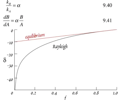
. Earlier we saw that for equilibrium fractionations, the fractionation factor is related to the equilibrium constant. For kinetic fractionations, the fractionation factor is simply the ratio of the rate constants, so that:

k

k

= ! 9.40

and dB

dA = ! ^B

A 9.41

Rearranging and integrating, we have:

ln B

B˚ = ! ln A A˚

or B

B˚ = A A˚

! "# $

%&

'

9.42

where A° and B° are the amount of A and B originally present. Dividing both sides by A/A°:

B / A

B° / A° = A A˚

! "# $

%&

' (1

9.43

Since the amount of B makes up only a trace of the total amount of H

O pre- sent, A is essentially equal to the total water present, and A/A° is essentially identical to ƒ, the fraction of the origi-

Figure 9.5. Fractionation of isotope ratios during Rayleigh

and equilibrium condensation. δ is the per mil difference

between the isotopic composition of original vapor and the

isotopic composition when fraction ƒ of the vapor remains.

W . M . W h i t e G e o c h e m i s t r y Chapter 9: Stable Isotopes

nal water remaining. Hence:

B / A

B° / A° = f

9.44

Subtracting 1 from both sides, we have: B / A – B° / A°

B° / A° = f

" 1 9.45

The left side of 9.45 is the relative deviation from the initial ratio. The permil relative deviation is sim- ply:

Δ = 1000(ƒ

– 1) 9.46

Of course, the same principle applies when water condenses from vapor. Assuming a value of α of 1.01, δ will vary with ƒ, the fraction of vapor remaining, as shown in Figure 9.5.

Even if the vapor and liquid remain in equilibrium through the condensation process, the isotopic composition of the remaining vapor will change continuously. The relevant equation is:

! = 1 " 1

(1 " f ) / # + f

$

%&

'

() * 1000 9.47

The effect of equilibrium condensation is also shown in Figure 9.5.

9.2.3 Mass Dependent and Mass Independent Fractionations

Oxygen and sulfur have both have more than two isotopes, as do, of course, many other elements.

How do we expect the fractionations between various isotope ratios to be related? For example, if a 4‰ fractionation of δ

O is observed in a particular sample, what value of δ

O do we predict? A first guess might be that we would expect the difference in the fractionation to be proportional to the mass difference. In other words, if δ

O is increased by 4‰ in some process, we would expect δ

O to be in- creased by about 2‰. If we think about this in a little more detail, we realize that fractionation factors are more complex functions of mass. Looking at equation 9.26, for example, we see that mass occurs in a variety of ways, as m

, as reduced mass, and complexly in the exponential term. Consequently, the ratio of fractionation of

O/

O to that of

O/

O won’t be exactly ½. In fact, in almost all cases the ra- tio is, on average, about 0.52. Thus the fractionation between isotopes does seem to be proportional to the difference in mass – this is referred to as mass dependent fractionation.

There are, however, some exceptions where the ratio of fractionation of

O/

O to that of

O/

O is close to 1. Since the extent of fractionation in these cases seems independent of the mass difference, this is called mass independent fractionation. Mass independent fractionation is rare. It was first observed oxygen isotope ratios in meteorites (see Chapter 10) and has subsequently been observed in oxygen iso- tope ratios of atmospheric gases, most dramatically in stratospheric ozone (Figure 9.6), and most re- cently in sulfur isotope ratios of Archean sediments and modern sulfur-bearing aerosols in ice. The causes of mass independent fractionation are poorly understood and it seems likely there may be more than one cause.

There is at least a partial theoretical explanation in the case of atmospheric ozone (Gao and Marcus, 2001). Their theory can be roughly explained as follows. Formation of ozone in the stratosphere typi- cally involves the energetic collision of monatomic and molecular oxygen, i.e.:

O + O

→ O

The ozone molecule thus formed is in an vibrationally excited state and, consequently, subject to disso-

ciation if it cannot loose this excess energy. The excess vibrational energy can be lost either by collisions

with other molecules, or by partitioning to rotational energy. In the stratosphere, collisions infrequent

compared hence repartitioning of vibrational energy represents an important pathway to stability. Be-

cause there are more possible energy transitions for asymmetric species such as

O

O

O and

O

O

O

than symmetric ones such as

O

O

O, the latter is repartition its excess energy and form a stable

molecule. At higher pressures, such as prevail in the troposphere, the symmetric molecule can loose

energy through far more frequent collisions, lessening the importance of the vibrational to rotational

W . M . W h i t e G e o c h e m i s t r y Chapter 9: Stable Isotopes

energy conversion. Gao and Marcus (2001) were able to closely match observed experimental fraction- ations, but their approach was in part empirical because a fully quantum mechanical treatment is not yet possible.

Theoretical understanding of mass independent sulfur isotope fractionations is less advanced. Mass independent fractionations similar to those observed (discussed below) have been produced in the laboratory by photo dissociation (photolysis) of SO

and SO using deep ultraviolet radiation (wave- lengths <220 nm). Photolysis at longer wavelengths does not produce mass independent fraction- ations. Current explanations therefore focus on ultraviolet photolysis. However, there as yet is no theo- retical explanation of this effect and alternative explanations, including ones that involve the role in symmetry in a manner analogous to ozone, cannot be entirely ruled out.

9.3 Isotope Geothermometry

One of the principal uses of stable iso- topes is geothermometry. Like “conven- tional” chemical geothermometers, stable isotope geothermometers are based on the temperature dependence of the equilibrium constant. As we have seen, this dependence may be expressed as:

ln K = ln ! = A + B

T

9.48

In actuality, the constants A and B are slowly varying functions of temperature, such that K tends to zero at absolute 0, corresponding to complete separation, and to 1 at infinite temperature, corresponding to no isotope separation. We can obtain a qualitative un- derstanding of why this as so by recalling

Table 9.2. Coefficients for Oxygen Isotope Fractionation at Low Temperatures ^:

∆ _Q

- φ = A + B × 10

/T

φ Α Β

Feldspar 0 0.97 + 1.04b*

Pyroxene 0 2.75

Garnet 0 2.88

Olivine 0 3.91

Muscovite –0.60 2.2

Amphibole –0.30 3.15

Biotite –0.60 3.69

Chlorite –1.63 5.44

Ilmenite 0 5.29

Magnetite 0 5.27

* b is the mole fraction of anorthite in the feldspar. This term therefore accounts for the compositional dependence discussed above. From Javoy (1976).

Figure 9.6. Oxygen isotopic composition in the stratosphere and troposphere show the effects of

mass independent fractionation. A few other atmospheric trace gases show similar effects. Es-

sentially all other material from the Earth and Moon plot on the terrestrial fractionation line.

W . M . W h i t e G e o c h e m i s t r y Chapter 9: Stable Isotopes

that the entropy of a system increases with temperature. At infinite tempera- ture, there is complete disorder, hence isotopes would be mixed randomly be- tween phases (ignoring for the moment the slight problem that at infinite tem- perature there would be neither phases nor isotopes). At absolute 0, there is perfect order, hence no mixing of iso- topes between phases. A and B are, however, sufficiently invariant over a limited range temperatures that they can be viewed as constants. We have also noted that at low temperatures, the form of equation 9.48 changes to K

∝ 1/T.

In principal, a temperature may be calculated from the isotopic fractiona-

tion between any two phases provided the phases equilibrated and the temperature dependence of the fractionation factor is known. And indeed, there are too many isotope geothermometers for all of them to be mentioned here. Figure 9.7 shows some fractionation factors between quartz and other minerals as a function of temperature. Figure 9.8 shows sulfur isotope fractionation factors be- tween various sulfur-bearing species and H

S.

Table 9.2 lists coefficients A and B for equa- tion 9.48 for the oxygen isotope fractionation factor between quartz and other oxides and silicates.

Because of the dependence of the equilib- rium constant on the inverse square of tem- perature, stable isotope geothermometry is employed primarily at low temperatures, that is, non-magmatic temperatures. At tempera- tures in excess of 800°C or so, the frac- tionations are generally small, making accu- rate temperatures difficult to determine from them. However, even at temperatures of the upper mantle (1000°C or more), fractiona- tions, although small, remain significant. Ex- perimentally determined fractionation factors for minerals in the temperature range of 600°

to 1300°C, which agree well with theoretical calculations, are given in Table 9.3.

Table 9.4 lists similar coefficients for the sulfur fractionation between H

S and sulfur- bearing compounds. Recall that if phases α and γ and α and β are in equilibrium with each other, then γ is also in equilibrium with β. Thus these tables may be used to obtain the fractionation between any two of the phases listed.

All geothermometers are based on the ap- Figure 9.7. Oxygen isotope fractionation for several

mineral pairs as a function of temperature.

Table 9.3 Coefficients for Oxygen Isotope Fractionations at Elevated Temperatures (600˚

- 1300˚C)

Cc Ab An Di Fo Mt

Qz 0.38 0.94 1.99 2.75 3.67 6.29

Cc 0.56 1.61 2.37 3.29 5.91

Ab 1.05 1.81 2.73 5.35

An 0.76 1.68 4.30

Di 0.92 3.54

Fo 2.62

Coefficients are for mineral pair fractionations expressed as

1000α = B × 10

/T

where B is given in the Table. Qz: quartz,

Cc: calcite, Ab: albite, An: anorthite, Di: diopside, Fo: forsterite,

Mt: magnetite. For example, the fractionation between albite

and diopside is 1000α

= 1.81×10

/T

(T in kelvins). From

Chiba et al. (1989).

W . M . W h i t e G e o c h e m i s t r y Chapter 9: Stable Isotopes

parently contradictory assumptions that com- plete equilibrium was achieved between phases during, or perhaps after, formation of the phases, but that the phases did not re-equilibrate when they subsequently cooled. The reason these as- sumptions can be made and geothermometry works at all is the exponential dependence of re- action rates on temperature that we discussed in Chapter 5. Isotope geothermometers have the same implicit assumptions about the achieve- ment of equilibrium as other geothermometers.

The importance of the equilibrium basis of geothermometry must be emphasized. Because most stable isotope geothermometers (though not all) are applied to relatively low temperature situations, violation of the assumption that com- plete equilibrium was achieved is not un- common. We have seen that isotopic fraction- ations may arise from kinetic as well as equilib-

rium effects. If reactions do not run to completion, the isotopic differences may reflect kinetic effects as much as equilibrium effects. There are other problems that can result in incorrect temperature as well;

for example, the system may partially re-equilibration at some lower temperature during cooling. A further problem with isotope geothermometry is that free energies of the exchange reactions are rela- tively low; meaning there is little chemical en-

ergy available to drive the reaction. Indeed, isotopic equilibrium probably often depends on other reactions occurring that mobilize the element involved in the exchange. Solid-state exchange reactions will be particularly slow at temperatures well below the melting point.

Equilibrium between solid phases will thus generally depend on reaction of these phases with a fluid. This latter point is true of ‘conven- tional’ geothermometers as well, and metamor- phism, one of the important areas of appli- cation of isotope geothermometry, generally occurs in the presence of a fluid.

Isotope geothermometers do have several advantages over conventional chemical ones.

First, as we have noted, there is no volume change associated with isotopic exchange reac- tions and hence no pressure dependence of the equilibrium constant. However, Rumble has suggested an indirect pressure dependence, wherein the fractionation factor depends on fluid composition, which in turn depends on pressure. Second, whereas conventional chemical geothermometers are generally based on solid solution, isotope geothermometers can make use of pure phases such as SiO

, etc.

Generally, any dependence on the composition of phases involved is of relatively second order

Table 9.4. Coefficients for Sulfur Isotope Fractionation:

∆ φ -H

S = A × 10

/T

+ B × 10

/T (T in kelvins )

φ Β A T°C

Range

CaSO

6.0±0.5 5.26 200-350

SO

–5±0.5 4.7 350-1050

FeS

0.4±0.08 200-700

ZnS 0.10±0.05 50-705

CuS –0.4±0.1

Cu

S –0.75±0.1

SnS –0.45±0.1

MoS

0.45±0.1

Ag

S –0.8±0.1

PbS –0.63±0.05 50-700

From Ohmoto and Rye (1979)

Figure 9.8. Relationship of S isotope fractionation

between H

S and other sulfur-bearing species and

temperature.