Assessing Data Quality –
A Probability-based Metric for Semantic Consistency
Authors:
Heinrich, Bernd, Department of Management Information Systems, University of Regensburg, Universitätsstr. 31, 93053 Regensburg, Germany, Bernd.Heinrich@ur.de Klier, Mathias, Institute of Technology and Process Management, University of Ulm, Helmholtzstr. 22, 89081 Ulm, Germany, Mathias.Klier@uni-ulm.de
Schiller, Alexander, Department of Management Information Systems, University of Regensburg, Universitätsstr. 31, 93053 Regensburg, Germany, Alexander.Schiller@ur.de Wagner, Gerit, Department of Management Information Systems, University of Regensburg, Universitätsstr. 31, 93053 Regensburg, Germany, Gerit.Wagner@ur.de
© 2018. This manuscript version is made available under the CC-BY-NC-ND 4.0 license http://creativecommons.org/licenses/by-nc-nd/4.0/
Citation: Bernd Heinrich, Mathias Klier, Alexander Schiller, Gerit Wagner, Assessing Data Quality –
A Probability-based Metric for Semantic Consistency, Decision Support Systems,Volume 110, June 2018, Pages 95-106, ISSN 0167-9236, DOI 10.1016/j.dss.2018.03.011
(https://www.sciencedirect.com/science/article/pii/S0167923618300599)
Assessing Data Quality –
A Probability-based Metric for Semantic Consistency
Abstract:
We present a probability-based metric for semantic consistency using a set of uncertain rules. As opposed to existing metrics for semantic consistency, our metric allows to consider rules that are expected to be fulfilled with specific probabilities. The resulting metric values represent the probability that the assessed dataset is free of internal contradictions with regard to the uncertain rules and thus have a clear interpretation. The theoretical basis for determining the metric values are statistical tests and the concept of the p-value, allowing the interpretation of the metric value as a probability. We demonstrate the practical applicability and effectiveness of the metric in a real-world setting by analyzing a customer dataset of an insurance company. Here, the metric was applied to identify semantic consistency problems in the data and to support decision-making, for instance, when offering individual products to customers.
Keywords: data quality, data quality assessment, data quality metric, data consistency
1 Introduction
Making use of large amounts of internal and external data becomes increasingly important for companies to gain competitive advantage and enable data-driven decisions in businesses (Ngai, Gunasekaran, Wamba, Akter, & Dubey, 2017). However, data quality problems still impede companies to generate the best value from data (Moges, van Vlasselaer, Lemahieu, & Baesens, 2016; Witchalls, 2014). Overall, poor data quality amounts to an average financial impact of $9.7 million per year and organization as reported by recent Gartner research (Moore, 2017). In particular, 63% of the respondents of a survey by Moges, Dejaeger, Lemahieu, and Baesens (2011, p. 639) indicated that “inconsistency (value and format) and diversity of data sources are main recurring challenges of data quality”.
Data quality can be defined as the “agreement between the data views presented by an information system and that same data in the real world” (Orr, 1998, p. 67). In this regard, data quality
is a multidimensional construct comprising different dimensions such as accuracy, consistency, completeness, and currency (Batini & Scannapieco, 2016; Redman, 1996; Zak & Even, 2017). In the following, we focus on consistency, in particular semantic consistency, as one of the most important dimensions (Blake & Mangiameli, 2011; Shankaranarayanan, Iyer, & Stoddard, 2012; Wand & Wang, 1996). We define semantic consistency as the degree to which assessed data is free of internal contradictions (cf. also Batini & Scannapieco, 2016; Heinrich, Kaiser, & Klier, 2007; Redman, 1996).
Contradictions are usually determined based on a set of rules (Batini & Scannapieco, 2006;
Heinrich et al., 2007; Mezzanzanica, Cesarini, Mercorio, & Boselli, 2012). Thereby, a rule represents a proposition consisting of two logical statements, where the first statement (antecedent) implies the second (consequent). For instance, in a database containing master data about customers in Western Europe, such a rule may be 𝑦𝑒𝑎𝑟 𝑜𝑓 𝑏𝑖𝑟𝑡ℎ = 2003 → 𝑚𝑎𝑟𝑖𝑡𝑎𝑙 𝑠𝑡𝑎𝑡𝑢𝑠 = 𝑠𝑖𝑛𝑔𝑙𝑒. Stored customer data regarding a married customer born in 2003 would contradict this rule, indicating a consistency problem.
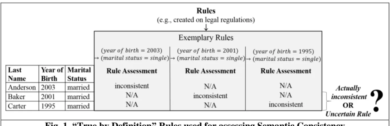
Existing data quality metrics for semantic consistency are based on rules which are considered as “true by definition” (cf. Section 2). This means that the rules have to be true for all of the assessed data and any violation indicates inconsistent data. Examples for such rules are provided in Figure 1, which also shows some selected records of a customer database serving as a basis for our discussion:
Fig. 1. “True by Definition” Rules used for assessing Semantic Consistency
Due to the fact that in Western Europe marriage is only legally allowed for people of age 16 and older, for an assessment in the year 2018, a value for year of birth of 2003 (antecedent of the first rule in Figure 1) implies the value single for marital status (consequent of the first rule), which is a typical example for a “true by definition” rule. In this case, the value married for marital status of the first record is assessed as inconsistent. However, for the assessment of semantic consistency it can be necessary to also consider rules such as 𝑦𝑒𝑎𝑟 𝑜𝑓 𝑏𝑖𝑟𝑡ℎ = 2001 → 𝑚𝑎𝑟𝑖𝑡𝑎𝑙 𝑠𝑡𝑎𝑡𝑢𝑠 = 𝑠𝑖𝑛𝑔𝑙𝑒 (second
rule in Figure 1). Here, one has to distinguish: On the one hand, violations of such a rule – assessed in 2018 – may indeed indicate an erroneous value which could have resulted from a random or systematic data error (cf. Alkharboush & Yuefeng Li, 2010; Fisher, Lauria, & Matheus, 2009). On the other hand, violations may stem from the fact that the rule is not “true by definition”, but only fulfilled with a specific probability. For example, some customers may indeed have married at the age of 16. Therefore, a violation of this rule does not necessarily imply that such data is inconsistent and of low quality. This also holds for other years of birth (e.g., 𝑦𝑒𝑎𝑟 𝑜𝑓 𝑏𝑖𝑟𝑡ℎ = 1995; third rule in Figure 1) or, in general, for other antecedents and consequents or applications where rules cannot be considered as “true by definition”. Hence, we are confronted with rules with uncertain consequent, to which we refer as uncertain rules in the following. To the best of our knowledge, none of the existing approaches aiming to measure semantic consistency has considered such relevant uncertain rules yet.
Thus, to (1) consider uncertain rules in a well-founded way and (2) ensure a clear interpretation of the resulting metric values, we propose a data quality metric for semantic consistency based on probability theory. To address uncertain rules, the metric delivers an indication rather than a statement under certainty regarding the degree to which assessed data is free of internal contradictions. We argue that the well-founded methods of probability theory are adequate and valuable to deal with uncertain rules. More precisely, the theoretical basis for determining the metric values are statistical tests and the concept of the p-value, allowing the clear interpretation of the metric values as probabilities.
The remainder of the paper is structured as follows. In the next section, we discuss related work and the research gap. Then, we present a probability-based metric for semantic consistency and outline possible ways to instantiate this metric. In the fourth section, we illustrate the case of an insurance company to demonstrate the practical applicability and effectiveness of the metric. Finally, we briefly summarize the findings and conclude with a discussion of limitations and directions for further research.
2 Related Work
The data quality dimension consistency is seen “as a multi-faceted dimension” (Blake & Mangiameli, 2009, p. 3) which can be defined in terms of representational consistency, integrity, and semantic consistency (Blake & Mangiameli, 2009). Since these three aspects stem from different domains, they
overlap in some cases. Representational consistency requires that data are “presented in the same format and are compatible with previous data” (Blake & Mangiameli, 2009; Wang & Strong, 1996). Integrity is often defined as entity, referential, domain, column, and user-defined integrity (Blake & Mangiameli, 2009; Lee, Pipino, Strong, & Wang, 2004). Entity integrity requires that data values considered as primary keys are unique and different from NULL. Referential integrity states that, given two relations, if an attribute is a primary key in one of them and is contained as a foreign key in the other one, the non- NULL data values from the second relation must be contained in the first one (Lee et al., 2004). Domain and column integrity require data values to be part of a predefined domain (e.g., 𝑖𝑛𝑐𝑜𝑚𝑒 ∈ ℝ+) and user-defined integrity requires the satisfaction of a set of general rules. Finally, semantic consistency refers to the absence of contradictions between different data values based on a rule set (Blake
& Mangiameli, 2009; Heinrich et al., 2007; Lee, Pipino, Funk, & Wang, 2006; Liu & Chi, 2002; Mecella et al., 2002; Mezzanzanica et al., 2012; Redman, 1996; Scannapieco, Missier, & Batini, 2005).
Generally, semantic consistency is equivalent to user-defined integrity.
In this paper, we focus on semantic consistency due to two reasons. First, assuring semantic consistency is crucial for decision support, as decision-making is typically based on data values. Second, both representational consistency and integrity have already been extensively studied in literature (Blake
& Mangiameli, 2009, 2011). Semantic consistency, however, is a field of research which gains more and more importance in the course of growing data volumes and their thorough analysis.
Underlining this importance, literature discusses several data quality problems and root causes which lead to inconsistencies with respect to data values (Kim, Choi, Hong, Kim, & Lee, 2003;
Laranjeiro, Soydemir, & Bernardino, 2015; Oliveira, Rodrigues, & Henriques, 2005; Rahm & Do, 2000;
Singh & Singh, 2010). These root causes are typically categorized in two ways. First, referring to the steps in the data management process (i.e., data entry/capturing, data transformation, data aggregation, data processing, etc.). And second, whether inconsistencies are caused by a single source or by multiple sources. Given this, a common and highly relevant root cause for inconsistencies are error-prone operative data entries via one single source (cf. Rahm & Do, 2000; Singh & Singh, 2010). This may be, for example, a call center employee, the person himself referred to in the considered record (e.g., a customer entering master data via a web application) or a damaged data capturing device (e.g., a
malfunctioning sensor). In all these scenarios, inconsistencies regarding, for instance, two data values of a customer record may arise. In the case of a call center employee or the customer himself, it is possible that only one of the two data values is correctly entered or changed. The second data value, however, may be entered or changed erroneously (or not at all). For instance, the value for 𝑦𝑒𝑎𝑟 𝑜𝑓 𝑏𝑖𝑟𝑡ℎ may be correctly entered as 2003, the value for 𝑚𝑎𝑟𝑖𝑡𝑎𝑙 𝑠𝑡𝑎𝑡𝑢𝑠, however, may be erroneously entered as 𝑚𝑎𝑟𝑟𝑖𝑒𝑑. Similarly, parts of a customer’s address may be entered incorrectly, leading to an inconsistency. A second prevalent root cause concerns the steps data aggregation and integration in the data management process with respect to multiple sources (e.g., different databases;
cf. Rahm & Do, 2000; Singh & Singh, 2010). Here, contradictory data values of, for instance, customer records may arise in scenarios in which the same customers are stored in multiple databases of departments and units of a company (e.g., after a merger). Contradictions may result from the integration of attributes or their values, for example when databases are integrated for a coordinated and comprehensive customer management. For instance, in one database, the 𝑚𝑎𝑟𝑖𝑡𝑎𝑙 𝑠𝑡𝑎𝑡𝑢𝑠 of a customer may be stored as 𝑠𝑖𝑛𝑔𝑙𝑒, but in a second database, the value for 𝑛𝑎𝑚𝑒 𝑜𝑓 𝑠𝑝𝑜𝑢𝑠𝑒 of the same customer may not be equal to NULL, indicating that the customer is 𝑚𝑎𝑟𝑟𝑖𝑒𝑑. Faulty business rules used for data transformation and leading to contradicting data values (cf. Singh & Singh, 2010) constitute another important scenario and root cause among many others, stressing the relevance of semantic consistency.
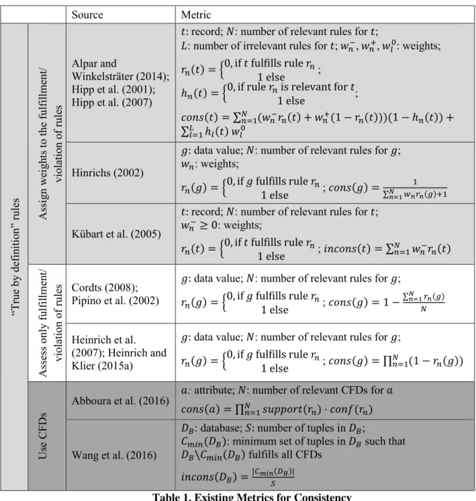
In the following, for reasons of simplicity, we will use the term consistency instead of semantic consistency. To provide an overview of existing works on metrics for consistency, we concentrate on metrics that are (i) formally defined (e.g., by a closed-form mathematical function) and (ii) result in a numerical metric value representing the consistency of the data values to be assessed. In that sense, we do not consider approaches that aim to identify potentially (in)consistent data values without providing numerical metric values for (in)consistency (e.g., Bronselaer, Nielandt, Mol, & Tré, 2016; Fan, Geerts, Tang, & Yu, 2013; Mezzanzanica et al., 2012). Table 1 presents existing metrics for consistency satisfying (i) and (ii). They follow the idea that consistency of data values can be determined based on the number of fulfilled rules, with a higher number of fulfilled rules implying higher consistency.
We discuss these metrics with regard to (1) the way they assess consistency and (2) the interpretation of the resulting metric values. Related to (1) the first three rows of Table 1 with the light
grey background contain metrics that assign weights to the fulfillment and violation of rules. The next two rows with the white background provide metrics assessing consistency purely as “true” or “false”
regarding the fulfillment and violation of rules. The last two rows with the dark grey background contain metrics relying on conditional functional dependencies (CFDs; Bohannon, Fan, Geerts, Jia, &
Kementsietsidis, 2007; Cong, Fan, Geerts, Jia, & Ma, 2007).
Source Metric
“True by definition” rules Assign weights to the fulfillment/ violation of rules
Alpar and
Winkelsträter (2014);
Hipp et al. (2001);
Hipp et al. (2007)
𝑡: record; 𝑁: number of relevant rules for 𝑡;
𝐿: number of irrelevant rules for 𝑡; 𝑤𝑛−, 𝑤𝑛+, 𝑤𝑙0: weights;
𝑟𝑛(𝑡) = {0, if 𝑡 fulfills rule 𝑟𝑛 1 else ; ℎ𝑛(𝑡) = {0, if rule 𝑟𝑛 is relevant for 𝑡
1 else ;
𝑐𝑜𝑛𝑠(𝑡) = ∑𝑁𝑛=1(𝑤𝑛−𝑟𝑛(𝑡) + 𝑤𝑛+(1 − 𝑟𝑛(𝑡)))(1 − ℎ𝑛(𝑡)) +
∑𝐿𝑙=1ℎ𝑙(𝑡) 𝑤𝑙0
Hinrichs (2002)
𝑔: data value; 𝑁: number of relevant rules for 𝑔;
𝑤𝑛: weights;
𝑟𝑛(𝑔) = {0, if 𝑔 fulfills rule 𝑟𝑛
1 else ; 𝑐𝑜𝑛𝑠(𝑔) = 1
∑𝑁𝑛=1𝑤𝑛𝑟𝑛(𝑔)+1
Kübart et al. (2005)
𝑡: record; 𝑁: number of relevant rules for 𝑡;
𝑤𝑛−≥ 0: weights;
𝑟𝑛(𝑡) = {0, if 𝑡 fulfills rule 𝑟𝑛
1 else ; 𝑖𝑛𝑐𝑜𝑛𝑠(𝑡) = ∑𝑁𝑛=1𝑤𝑛−𝑟𝑛(𝑡)
Assess only fulfillment/ violation of rules Cordts (2008);
Pipino et al. (2002)
𝑔: data value; 𝑁: number of relevant rules for 𝑔;
𝑟𝑛(𝑔) = {0, if 𝑔 fulfills rule 𝑟𝑛
1 else ; 𝑐𝑜𝑛𝑠(𝑔) = 1 −∑𝑁𝑛=1𝑟𝑛(𝑔)
𝑁
Heinrich et al.
(2007); Heinrich and Klier (2015a)
𝑔: data value; 𝑁: number of relevant rules for 𝑔;
𝑟𝑛(𝑔) = {0, if 𝑔 fulfills rule 𝑟𝑛
1 else ; 𝑐𝑜𝑛𝑠(𝑔) = ∏𝑁𝑛=1(1 − 𝑟𝑛(𝑔))
Use CFDs Abboura et al. (2016) 𝑎: attribute; 𝑁: number of relevant CFDs for 𝑎 𝑐𝑜𝑛𝑠(𝑎) = ∏𝑁𝑛=1𝑠𝑢𝑝𝑝𝑜𝑟𝑡(𝑟𝑛)⋅ 𝑐𝑜𝑛𝑓(𝑟𝑛)
Wang et al. (2016)
𝐷𝐵: database; 𝑆: number of tuples in 𝐷𝐵;
𝐶𝑚𝑖𝑛(𝐷𝐵): minimum set of tuples in 𝐷𝐵 such that 𝐷𝐵\𝐶𝑚𝑖𝑛(𝐷𝐵) fulfills all CFDs
𝑖𝑛𝑐𝑜𝑛𝑠(𝐷𝐵) =|𝐶𝑚𝑖𝑛(𝐷𝐵)|
𝑆
Table 1. Existing Metrics for Consistency
All metrics in the first three rows of Table 1 (Alpar & Winkelsträter, 2014; Hinrichs, 2002; Hipp et al., 2001; Hipp et al., 2007; Kübart et al., 2005) assign weights to the fulfillment and violation of rules. The considered rules correspond to association rules. For a given set of records, association rules are implications of the form 𝑋 → 𝑌 that satisfy specified constraints regarding minimum support and
minimum confidence (cf. Agrawal, Imieliński, & Swami, 1993; Srikant & Agrawal, 1996). Thereby, rule support 𝑠𝑢𝑝𝑝(𝑋 → 𝑌) is defined as the fraction of records that fulfill both antecedent 𝑋 and consequent 𝑌 of the rule; rule confidence 𝑐𝑜𝑛𝑓(𝑋 → 𝑌) denotes the fraction of records fulfilling the antecedent 𝑋 that also fulfill the consequent 𝑌 (cf. Agrawal et al., 1993). An example of an association rule is 𝑦𝑒𝑎𝑟 𝑜𝑓 𝑏𝑖𝑟𝑡ℎ = 1995 → 𝑚𝑎𝑟𝑖𝑡𝑎𝑙 𝑠𝑡𝑎𝑡𝑢𝑠 = 𝑠𝑖𝑛𝑔𝑙𝑒. If 80% of the records in the database with 𝑦𝑒𝑎𝑟 𝑜𝑓 𝑏𝑖𝑟𝑡ℎ = 1995 also fulfill 𝑚𝑎𝑟𝑖𝑡𝑎𝑙 𝑠𝑡𝑎𝑡𝑢𝑠 = 𝑠𝑖𝑛𝑔𝑙𝑒 and 5% of the records fulfill both 𝑦𝑒𝑎𝑟 𝑜𝑓 𝑏𝑖𝑟𝑡ℎ = 1995 and 𝑚𝑎𝑟𝑖𝑡𝑎𝑙 𝑠𝑡𝑎𝑡𝑢𝑠 = 𝑠𝑖𝑛𝑔𝑙𝑒, it follows that the support of the rule is 5%
while its confidence is 80%. To treat the violation of distinct association rules 𝑟𝑛 as differently severe when assessing consistency, for example Alpar and Winkelsträter (2014) and Hipp et al. (2007) use the rule confidence 𝑐𝑜𝑛𝑓( 𝑟𝑛) to determine respective weights. In particular, the idea of these authors is to assign a weight of 𝑐𝑜𝑛𝑓( 𝑟𝑛) to the fulfillment of a rule and a weight of −𝑐𝑜𝑛𝑓( 𝑟𝑛) to its violation. In order to determine consistency concerning several rules and a set of data values, the weights are calibrated and summed up.
While these approaches treat the violation of distinct rules as differently severe (i.e., depending on rule confidence), they assess the fulfillment of a rule to always be an indicator for high consistency by assigning a positive weight (i.e., 𝑐𝑜𝑛𝑓( 𝑟𝑛)) to rule fulfillments and vice versa. As only association rules above a chosen minimum threshold for confidence based on the dataset to be assessed are determined, rules below this threshold remain unconsidered in these approaches. However, rules with a lower confidence are also highly relevant for assessing consistency, as they can be an important indicator for inconsistent data. For example, a rule (confidence) stating that 30% of 17-year-olds are stored as being married would certainly help to identify inconsistencies because a much smaller percentage of 17- year-olds is actually married in Western Europe. In addition, solely using the rule confidence based on the assessed data can lead to misleading results if a large part of the data to be assessed is erroneous:
For instance, if 90% of all 17-year-olds are erroneously stored as being married in a database, a corresponding association rule and its rule confidence is determined (given a minimum rule confidence of e.g. 80%). On this basis, however, the 10% of 17-year-olds which are accurately stored as not being married would be considered as inconsistent. More generally, these approaches assess all rules with high confidence as “true by definition” and penalize violations against them as inconsistent.
To conclude, these metrics provide first, promising steps concerning the treatment of violations of distinct rules as differently severe. However, rules with low confidence are ignored and rules with high confidence are seen as “true by definition”. Further, the resulting values of these metrics suffer from a lack of clear interpretation (cf. (2)). Indeed, it remains unclear what a particular metric value actually means, obstructing its use for decision support. This is due to the summation of the (calibrated) weights (representing the rule confidences as “measures of consistency”). To illustrate this, we again consider the example of a customer database. A customer record may fulfill some association rules (e.g., the values for zip code and city) and violate others (e.g., the values for marital status and year of birth).
The respective calibrated weights are summed up, but the result of the summation is a real number with no clear interpretation (e.g., in terms of a probability whether the considered record is consistent).
Furthermore, the metric values are, in general, not interval-scaled and do not have a defined minimum and maximum. This may seriously hinder their usefulness for decision support: For example, in a second assessment of the customer data at a later point in time, the mined association rules and their confidence can differ from the first assessment. Then, a higher (or lower) metric value of the same, unchanged record in the second assessment does not necessarily represent higher (or lower) actual consistency. In fact, the consistency of the record may still be the same.
The metrics in the next two rows of Table 1 with the white background (Cordts, 2008; Heinrich et al., 2007; Heinrich & Klier, 2015a; Pipino et al., 2002) assess the consistency of data values only by
“true” or “false” statements regarding the fulfillment and violation of the considered rules. On this basis, they provide a clear interpretation of the metric values in terms of the percentage of data values consistent with respect to the considered rules (cf. (2)). These approaches, however, treat all rules equally as “true by definition” and thus have similar limitations as the metrics discussed above.
Finally, the metrics provided in the last two rows of Table 1 with the dark grey background (Abboura et al., 2016; Wang et al., 2016) assess consistency by using CFDs. A CFD is a pair (𝑋 → 𝑌, 𝑇𝑖) consisting of a functional dependency 𝑋 → 𝑌 (an implication of sets of attributes) and a certain tableau 𝑇𝑖 (with 𝑖 ∈ {1, 2, … , 𝑁}) which specifies values for the attributes in 𝑋 and 𝑌 (cf. Bohannon et al., 2007 for details). To give an example, stating that records with 𝑦𝑒𝑎𝑟 𝑜𝑓 𝑏𝑖𝑟𝑡ℎ = 1995 also fulfill 𝑚𝑎𝑟𝑖𝑡𝑎𝑙 𝑠𝑡𝑎𝑡𝑢𝑠 = 𝑠𝑖𝑛𝑔𝑙𝑒 can be represented by the following CFD: (𝑦𝑒𝑎𝑟 𝑜𝑓 𝑏𝑖𝑟𝑡ℎ →
𝑚𝑎𝑟𝑖𝑡𝑎𝑙 𝑠𝑡𝑎𝑡𝑢𝑠, 𝑇1), with 𝑇1 containing a row which includes 1995 as value for 𝑦𝑒𝑎𝑟 𝑜𝑓 𝑏𝑖𝑟𝑡ℎ and 𝑠𝑖𝑛𝑔𝑙𝑒 as value for 𝑚𝑎𝑟𝑖𝑡𝑎𝑙 𝑠𝑡𝑎𝑡𝑢𝑠. A probabilistic CFD is a pair consisting of a CFD and its confidence, where support and confidence of a probabilistic CFD are defined analogously to association rules (Golab, Karloff, Korn, Srivastava, & Yu, 2008). Abboura et al. (2016) define the consistency of an attribute to be the product of the support of a (probabilistic) CFD multiplied by its confidence. The product is taken over all CFDs relevant for the considered attribute. Thus, analogous to the approaches in the first three lines of Table 1, the approach assesses the considered CFDs as “true by definition” and penalizes violations against them as inconsistent. This results in similar problems as outlined above.
Additionally, the metric values do not provide a clear interpretation (cf. (2)). Wang et al. (2016) propose to determine a minimum subset of tuples in a database which – if corrected – would lead to the database fulfilling all CFDs. Then, the inconsistency of the database is measured by the ratio of the size of this minimum subset in relation to the size of the whole database.
Overall, existing metrics interpret their rules used for assessing consistency as “true by definition” resulting in several limitations. In particular, they do not deal with uncertain rules. Moreover, metrics which treat the violation of distinct rules as differently severe do not ensure a clear interpretation of the metric values. In the next section we address this research gap.
3 Probability-based Metric for Consistency
In this section, we present our metric for semantic consistency. First, we outline the general setting and the basic idea. Then, we describe methodological foundations which serve as a basis when defining the metric in the following subsection. Finally, we outline possible ways to instantiate the metric.
3.1 General Setting and Basic Idea
We consider the common relational database model and a database 𝐷𝐵 to be assessed. A relation consists of a set of attributes {𝑎1, 𝑎2, … , 𝑎𝑚} and a set of records 𝑇 = {𝑡1, 𝑡2, … , 𝑡𝑛}. The data value of record 𝑡𝑗 regarding attribute 𝑎𝑖 is denoted by 𝜙(𝑡𝑗, 𝑎𝑖). In line with existing literature (cf. Section 2), we use a rule set 𝑅 to assess consistency. Rules are propositions of the form 𝑟: 𝐴 → 𝐶, where 𝐴 (antecedent) and 𝐶 (consequent) are logical statements addressing either single attributes in 𝐷𝐵 or relations between them.
As opposed to existing approaches, we do not treat rules as “true by definition”. Rather, we aim to consider uncertain rules that are expected to be fulfilled with specific probabilities.
This allows to determine metric values which represent the probability that the assessed dataset is free of internal contradictions with regard to these uncertain rules. More precisely, for a data value 𝜙(𝑡𝑗, 𝑎𝑖) in 𝐷𝐵 and an uncertain rule 𝑟, we interpret consistency as the probability that 𝜙(𝑡𝑗, 𝑎𝑖) is free of contradictions with regard to 𝑟. A metric that results in a probability guarantees that the metric takes values in [0; 1] and the metric values have a clear interpretation.
The following running example from our application context (cf. Section 4) illustrates the idea of our metric: An insurer strives to conduct a product campaign targeting only married customers younger than 20 years. If the data stored in the customer database is of low quality, wrong decisions and economic losses may result. For instance, if a customer younger than 20 years is erroneously stored as married in the database, contacting him with a product offer will generate costs and may lead to lower customer satisfaction. In case the insurer aims to assess the consistency of its customer database before conducting the campaign, existing metrics for consistency would consider the rule 𝑟1: 𝑦𝑒𝑎𝑟 𝑜𝑓 𝑏𝑖𝑟𝑡ℎ >
1998 → 𝑚𝑎𝑟𝑖𝑡𝑎𝑙 𝑠𝑡𝑎𝑡𝑢𝑠 = 𝑠𝑖𝑛𝑔𝑙𝑒. This rule is selected because it is fulfilled by most people that are younger than 20 years (e.g., 95%), which goes along with a high rule confidence. However, such metrics would assess data regarding a married customer who is younger than 20 years as inconsistent. Thus, the determined metric values could not provide any support within the campaign.
Our metric, in contrast, additionally considers the rule 𝑟2: 𝑦𝑒𝑎𝑟 𝑜𝑓 𝑏𝑖𝑟𝑡ℎ > 1998 → 𝑚𝑎𝑟𝑖𝑡𝑎𝑙 𝑠𝑡𝑎𝑡𝑢𝑠 = 𝑚𝑎𝑟𝑟𝑖𝑒𝑑 and the probabilities with which 𝑟1 and 𝑟2 are expected to be fulfilled (e.g., based on census data). In particular, our approach evaluates the actual fulfillment of 𝑟1 and 𝑟2 in the customer database in comparison to the expected distribution of rule fulfillment. For example, the number of married people that are younger than 20 years is generally low, meaning that 𝑟2 is expected to be fulfilled only with a low frequency (e.g., 4.1%). Thus, if 𝑟2 is fulfilled similarly infrequently in the customer database (e.g., 4.2%), the corresponding data of married customers is assessed to have a high probability of being consistent.
This interpretation of metric values as probabilities is viable because statistical tests and the
concept of the p-value form the methodological foundation for determining the metric values (cf. Section 3.2). Moreover, by assessing consistency as a probability, the metric values for each customer can be integrated in decision support, for instance, into the calculation of expected values. Such a calculation may reveal that targeting a married customer younger than 20 years within the campaign is only beneficial if the consistency of the data of this customer – represented by a probability – is greater than 0.8. Thus, applying the rule 𝑟2, the metric can be used to determine whether this threshold is met (note that this threshold is totally different from rule confidence, as confidence of 𝑟2 is only 4.2%).
3.2 Methodological Foundations
3.2.1 Uncertain Rules
A rule 𝑟: 𝐴 → 𝐶 consists of logical statements 𝐴 and 𝐶, with 𝐴 and 𝐶 describing single attributes or relations between different attributes in 𝐷𝐵. The simplest form of a logical statement 𝑆 is defined as (Chiang & Miller, 2008; Fan et al., 2013):
< 𝑎𝑡𝑡𝑟𝑖𝑏𝑢𝑡𝑒 >< 𝑜𝑝𝑒𝑟𝑎𝑡𝑜𝑟 >< 𝑎𝑡𝑡𝑟𝑖𝑏𝑢𝑡𝑒 >
or (1)
< 𝑎𝑡𝑡𝑟𝑖𝑏𝑢𝑡𝑒 >< 𝑜𝑝𝑒𝑟𝑎𝑡𝑜𝑟 >< 𝑐𝑜𝑛𝑠𝑡𝑎𝑛𝑡 >
Here, < 𝑎𝑡𝑡𝑟𝑖𝑏𝑢𝑡𝑒 > is one of the attributes 𝑎𝑖 and < 𝑜𝑝𝑒𝑟𝑎𝑡𝑜𝑟 > is a binary operator such as =, ≥,
>, ≠ or 𝑠𝑢𝑏𝑠𝑡𝑟𝑖𝑛𝑔_𝑜𝑓. Simple logical statements can be linked by conjunction (AND, ∧), disjunction (OR, ∨) or negation (NOT, ¬) to form more complex logical statements. For instance, in the running example, we may have a rule of the following form:
𝑟3: 𝑦𝑒𝑎𝑟 𝑜𝑓 𝑏𝑖𝑟𝑡ℎ > 1998 ∧ 𝑔𝑒𝑛𝑑𝑒𝑟 = 𝑓𝑒𝑚𝑎𝑙𝑒 → 𝑚𝑎𝑟𝑖𝑡𝑎𝑙 𝑠𝑡𝑎𝑡𝑢𝑠 = 𝑠𝑖𝑛𝑔𝑙𝑒 (2) Here, 𝑦𝑒𝑎𝑟 𝑜𝑓 𝑏𝑖𝑟𝑡ℎ > 1998, 𝑔𝑒𝑛𝑑𝑒𝑟 = 𝑓𝑒𝑚𝑎𝑙𝑒, 𝑚𝑎𝑟𝑖𝑡𝑎𝑙 𝑠𝑡𝑎𝑡𝑢𝑠 = 𝑠𝑖𝑛𝑔𝑙𝑒, and 𝑦𝑒𝑎𝑟 𝑜𝑓 𝑏𝑖𝑟𝑡ℎ >
1998 ∧ 𝑔𝑒𝑛𝑑𝑒𝑟 = 𝑓𝑒𝑚𝑎𝑙𝑒 are logical statements. To determine whether a logical statement 𝑆 is true or false for a record 𝑡 of 𝐷𝐵, it can be applied to 𝑡 by replacing each attribute 𝑎𝑖 contained in 𝑆 by 𝜙(𝑡, 𝑎𝑖). In other words, the corresponding data values of the record are inserted. We further define the set of records in 𝐷𝐵 rendering 𝑆 true as 𝑓𝑢𝑙𝑓𝑖𝑙𝑙𝑖𝑛𝑔 𝑟𝑒𝑐𝑜𝑟𝑑𝑠(𝐷𝐵, 𝑆) ≔ {𝑡 ∈ 𝑇| 𝑆(𝑡) is 𝑡𝑟𝑢𝑒}.
As an example, we can apply the antecedent 𝑦𝑒𝑎𝑟 𝑜𝑓 𝑏𝑖𝑟𝑡ℎ > 1998 ∧ 𝑔𝑒𝑛𝑑𝑒𝑟 = 𝑓𝑒𝑚𝑎𝑙𝑒 and the consequent 𝑚𝑎𝑟𝑖𝑡𝑎𝑙 𝑠𝑡𝑎𝑡𝑢𝑠 = 𝑚𝑎𝑟𝑟𝑖𝑒𝑑 of the rule 𝑟3 to a record 𝑡 of the database 𝐷𝐵 with 𝜙(𝑡, 𝑦𝑒𝑎𝑟 𝑜𝑓 𝑏𝑖𝑟𝑡ℎ) = 2000, 𝜙(𝑡, 𝑔𝑒𝑛𝑑𝑒𝑟) = 𝑓𝑒𝑚𝑎𝑙𝑒 and 𝜙(𝑡, 𝑚𝑎𝑟𝑖𝑡𝑎𝑙 𝑠𝑡𝑎𝑡𝑢𝑠) = 𝑚𝑎𝑟𝑟𝑖𝑒𝑑. As
2000 > 1998, 𝑓𝑒𝑚𝑎𝑙𝑒 = 𝑓𝑒𝑚𝑎𝑙𝑒 and 𝑚𝑎𝑟𝑟𝑖𝑒𝑑 = 𝑚𝑎𝑟𝑟𝑖𝑒𝑑, it follows 𝐴(𝑡) 𝑡𝑟𝑢𝑒 and 𝐶(𝑡) 𝑡𝑟𝑢𝑒.
Thus, 𝑡 ∈ 𝑓𝑢𝑙𝑓𝑖𝑙𝑙𝑖𝑛𝑔 𝑟𝑒𝑐𝑜𝑟𝑑𝑠(𝐷𝐵, 𝐴) and 𝑡 ∈ 𝑓𝑢𝑙𝑓𝑖𝑙𝑙𝑖𝑛𝑔 𝑟𝑒𝑐𝑜𝑟𝑑𝑠(𝐷𝐵, 𝐶).
We call a rule 𝑟: 𝐴 → 𝐶 relevant for a record 𝑡 ∈ 𝑇 if 𝑡 ∈ 𝑓𝑢𝑙𝑓𝑖𝑙𝑙𝑖𝑛𝑔 𝑟𝑒𝑐𝑜𝑟𝑑𝑠(𝐷𝐵, 𝐴). If 𝑟 is relevant for 𝑡, we say that 𝑡 fulfills 𝑟, if 𝑡 ∈ 𝑓𝑢𝑙𝑓𝑖𝑙𝑙𝑖𝑛𝑔 𝑟𝑒𝑐𝑜𝑟𝑑𝑠(𝐷𝐵 , 𝐴 ∧ 𝐶), and that 𝑡 violates 𝑟 otherwise. As mentioned above, we consider uncertain rules and not just rules which are “true by definition”. To be more precise, an uncertain rule in our context is defined as:
(𝑟: 𝐴 → 𝐶, 𝑝(𝑟)) (3)
An uncertain rule (𝑟: 𝐴 → 𝐶, 𝑝(𝑟)) has two components. It comprises a rule 𝑟 containing the logical statements 𝐴 (antecedent) and 𝐶 (consequent) as well as a number 𝑝(𝑟) ∈ [0; 1] representing the probability with which 𝑟 is expected to be fulfilled. The probability 𝑝(𝑟) allows to specify the uncertainty of the rule 𝑟. In contrast to existing approaches, this allows to consider rules that are unlikely to be fulfilled as well as almost certain rules or rules which are “true by definition” (i.e., the special case 𝑝(𝑟) = 1) for the assessment of consistency. It is different from the confidence of an association rule as it is not based on the relative frequency of rule fulfillment in the dataset to be assessed. Moreover, the probability 𝑝(𝑟) is not used for selecting rules (e.g., with a high probability of being fulfilled), but rather for assessing consistency (the determination of uncertain rules will be outlined in Section 3.4.1).
3.2.2 Using Uncertain Rules for the Assessment of Consistency
Let 𝑟: 𝐴 → 𝐶 be a rule in the rule set 𝑅 and let 𝐷𝐵 be the dataset to be assessed. The rule 𝑟 is expected to be fulfilled with probability 𝑝(𝑟). Hence, if the records in 𝑓𝑢𝑙𝑓𝑖𝑙𝑙𝑖𝑛𝑔 𝑟𝑒𝑐𝑜𝑟𝑑𝑠(𝐷𝐵, 𝐴) are consistent with regard to 𝑟, the application of 𝑟 to such a record 𝑡 can be seen as a Bernoulli trial with success probability 𝑝(𝑟), where success is defined as 𝑡 ∈ 𝑓𝑢𝑙𝑓𝑖𝑙𝑙𝑖𝑛𝑔 𝑟𝑒𝑐𝑜𝑟𝑑𝑠(𝐷𝐵, 𝐴 ∧ 𝐶). This is, because applying 𝑟 to a record in 𝑓𝑢𝑙𝑓𝑖𝑙𝑙𝑖𝑛𝑔 𝑟𝑒𝑐𝑜𝑟𝑑𝑠(𝐷𝐵, 𝐴) has only two possible outcomes: The rule can either be fulfilled (with probability 𝑝(𝑟)) or violated (with probability 1 − 𝑝(𝑟)). Thus, the Bernoulli trial can be represented by a random variable 𝑟(𝑡) resulting in 𝑟(𝑡)~𝐵𝑒𝑟𝑛(𝑝(𝑟)):
𝑟(𝑡): = { 1 if 𝑡 ∈ 𝑓𝑢𝑙𝑓𝑖𝑙𝑙𝑖𝑛𝑔 𝑟𝑒𝑐𝑜𝑟𝑑𝑠(𝐷𝐵, 𝐴 ∧ 𝐶)
0 if 𝑡 ∉ 𝑓𝑢𝑙𝑓𝑖𝑙𝑙𝑖𝑛𝑔 𝑟𝑒𝑐𝑜𝑟𝑑𝑠(𝐷𝐵, 𝐴 ∧ 𝐶), 𝑡 ∈ 𝑓𝑢𝑙𝑓𝑖𝑙𝑙𝑖𝑛𝑔 𝑟𝑒𝑐𝑜𝑟𝑑𝑠(𝐷𝐵, 𝐴) (4) Similarly, 𝑟 can then be applied to all records 𝑡 in 𝐷𝐵 with 𝑡 ∈ 𝑓𝑢𝑙𝑓𝑖𝑙𝑙𝑖𝑛𝑔 𝑟𝑒𝑐𝑜𝑟𝑑𝑠(𝐷𝐵, 𝐴) and the
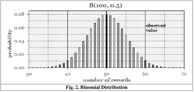
results can be summed up by the random variable 𝑋(𝑟): = ∑𝑡∈𝑓𝑢𝑙𝑓𝑖𝑙𝑙𝑖𝑛𝑔 𝑟𝑒𝑐𝑜𝑟𝑑𝑠(𝐷𝐵,𝐴)𝑟(𝑡). As a sum of independent Bernoulli-distributed random variables, 𝑋(𝑟) follows a binomial distribution with parameters |𝑓𝑢𝑙𝑓𝑖𝑙𝑙𝑖𝑛𝑔 𝑟𝑒𝑐𝑜𝑟𝑑𝑠(𝐷𝐵, 𝐴)| and 𝑝(𝑟): 𝑋(𝑟)~𝐵(|𝑓𝑢𝑙𝑓𝑖𝑙𝑙𝑖𝑛𝑔 𝑟𝑒𝑐𝑜𝑟𝑑𝑠(𝐷𝐵, 𝐴)|, 𝑝(𝑟)). An illustration for such a distribution with parameters 100 and 0.5 is presented in Figure 2.
Fig. 2. Binomial Distribution
If the records in 𝑓𝑢𝑙𝑓𝑖𝑙𝑙𝑖𝑛𝑔 𝑟𝑒𝑐𝑜𝑟𝑑𝑠(𝐷𝐵, 𝐴) are consistent with regard to 𝑟 and 𝑝(𝑟), it follows that
|𝑓𝑢𝑙𝑓𝑖𝑙𝑙𝑖𝑛𝑔 𝑟𝑒𝑐𝑜𝑟𝑑𝑠(𝐷𝐵, 𝐴 ∧ 𝐶)| is distributed as the successes of 𝑋(𝑟). Thus, to determine the consistency of the records in 𝑓𝑢𝑙𝑓𝑖𝑙𝑙𝑖𝑛𝑔 𝑟𝑒𝑐𝑜𝑟𝑑𝑠(𝐷𝐵, 𝐴), the actual value of
|𝑓𝑢𝑙𝑓𝑖𝑙𝑙𝑖𝑛𝑔 𝑟𝑒𝑐𝑜𝑟𝑑𝑠(𝐷𝐵, 𝐴 ∧ 𝐶)| is contrasted with the distribution of 𝑋(𝑟). In Figure 2, we observe
|𝑓𝑢𝑙𝑓𝑖𝑙𝑙𝑖𝑛𝑔 𝑟𝑒𝑐𝑜𝑟𝑑𝑠(𝐷𝐵, 𝐴 ∧ 𝐶)| = 60 and expected value 𝐸[𝑋(𝑟)] = 50, resulting in an indication of inconsistency.
Based on this idea, we develop a probability-based metric for consistency founded on the well- known concept of the (two-sided) p-value in hypothesis testing. Let 𝑝′(𝑟) be the relative frequency with which the rule 𝑟 is fulfilled by a relevant record in the dataset 𝐷𝐵. If the relevant records are consistent with regard to 𝑟, then 𝑝′(𝑟) should correspond to 𝑝(𝑟) (e.g., 0.5 in Figure 2). Thus, in statistical terms, measuring consistency implies testing the null hypothesis 𝐻0: 𝑝′(𝑟) = 𝑝(𝑟) against the alternative hypothesis 𝐻1: 𝑝′(𝑟) ≠ 𝑝(𝑟) for the binomially distributed random variable 𝑋(𝑟)~𝐵(|𝑓𝑢𝑙𝑓𝑖𝑙𝑙𝑖𝑛𝑔 𝑟𝑒𝑐𝑜𝑟𝑑𝑠(𝐷𝐵, 𝐴)|, 𝑝(𝑟)). A two-sided alternative hypothesis is used because both too many and too few fulfillments of 𝑟 indicate inconsistency: The more |𝑓𝑢𝑙𝑓𝑖𝑙𝑙𝑖𝑛𝑔 𝑟𝑒𝑐𝑜𝑟𝑑𝑠(𝐷𝐵, 𝐴 ∧ 𝐶)| deviates from 𝐸[𝑋(𝑟)], the more the consistency of 𝐷𝐵 decreases in regard to 𝑟.
This intuitive understanding is formalized by the two-sided p-value. It represents the probability that a value occurs under the null hypothesis which is equal to or more extreme than the observed value.
For example, in Figure 2, 𝐸[𝑋(𝑟)] = 50 and observed value |𝑓𝑢𝑙𝑓𝑖𝑙𝑙𝑖𝑛𝑔 𝑟𝑒𝑐𝑜𝑟𝑑𝑠(𝐷𝐵, 𝐴 ∧ 𝐶)| = 60.
Since the distribution is symmetric, values ≥ 60 and values ≤ 40 are equal to or more extreme than the observed value. Following this, the two-sided p-value is calculated by summing up the probabilities 𝑝(𝑋(𝑟) ≥ 60) and 𝑝(𝑋(𝑟) ≤ 40), represented by the dark grey bars.
In our case, the observed value is |𝑓𝑢𝑙𝑓𝑖𝑙𝑙𝑖𝑛𝑔 𝑟𝑒𝑐𝑜𝑟𝑑𝑠(𝐷𝐵, 𝐴 ∧ 𝐶)| and the expected value is 𝐸[𝑋(𝑟)]. Thus, the p-value represents the probability that, under the null hypothesis, the random variable 𝑋(𝑟) yields a value equal to or more extreme than |𝑓𝑢𝑙𝑓𝑖𝑙𝑙𝑖𝑛𝑔 𝑟𝑒𝑐𝑜𝑟𝑑𝑠(𝐷𝐵, 𝐴 ∧ 𝐶)|. Hence, it represents the probability that the assessed records in 𝐷𝐵 are free of contradictions with regard to the rule 𝑟. The two-sided p-value of the random variable 𝑋(𝑟)~𝐵(|𝑓𝑢𝑙𝑓𝑖𝑙𝑙𝑖𝑛𝑔 𝑟𝑒𝑐𝑜𝑟𝑑𝑠(𝐷𝐵, 𝐴)|, 𝑝(𝑟)) with respect to the observed value |𝑓𝑢𝑙𝑓𝑖𝑙𝑙𝑖𝑛𝑔 𝑟𝑒𝑐𝑜𝑟𝑑𝑠(𝐷𝐵, 𝐴 ∧ 𝐶)| is denoted as follows:
𝑝-𝑣𝑎𝑙𝑢𝑒(𝑋(𝑟)~𝐵(|𝑓𝑢𝑙𝑓𝑖𝑙𝑙𝑖𝑛𝑔 𝑟𝑒𝑐𝑜𝑟𝑑𝑠(𝐷𝐵, 𝐴)|, 𝑝(𝑟)), |𝑓𝑢𝑙𝑓𝑖𝑙𝑙𝑖𝑛𝑔 𝑟𝑒𝑐𝑜𝑟𝑑𝑠(𝐷𝐵, 𝐴 ∧ 𝐶)|) (5) Note that we are aware of the discussion regarding the p-value (cf., e.g., Goodman, 2008) and since this is not the main focus of our paper, we follow the above standard interpretation. The outlined methodological foundations allow for a formal definition of our metric in the next subsection and ensure a clear interpretation of the metric values.
3.3 Definition of the Metric for Consistency
Let 𝐷𝐵 be a database, 𝑡𝑗 ∈ 𝑇 be a record in 𝐷𝐵, 𝑎𝑖 be an attribute in 𝐷𝐵, and 𝑟: 𝐴 → 𝐶 with 𝑝(𝑟) ∈ [0; 1]
be an uncertain rule such that 𝑎𝑖 is part of 𝑟 and 𝑡𝑗∈ 𝑓𝑢𝑙𝑓𝑖𝑙𝑙𝑖𝑛𝑔 𝑟𝑒𝑐𝑜𝑟𝑑𝑠(𝐷𝐵, 𝐴 ∧ 𝐶). We define the consistency of the data value 𝜙(𝑡𝑗, 𝑎𝑖) with regard to 𝑟 as:
𝑄𝐶𝑜𝑛𝑠(𝜙(𝑡𝑗, 𝑎𝑖), 𝑟: 𝐴 → 𝐶):=
𝑝-𝑣𝑎𝑙𝑢𝑒(𝑋(𝑟)~𝐵(|𝑓𝑢𝑙𝑓𝑖𝑙𝑙𝑖𝑛𝑔 𝑟𝑒𝑐𝑜𝑟𝑑𝑠(𝐷𝐵, 𝐴)|, 𝑝(𝑟)), |𝑓𝑢𝑙𝑓𝑖𝑙𝑙𝑖𝑛𝑔 𝑟𝑒𝑐𝑜𝑟𝑑𝑠(𝐷𝐵, 𝐴 ∧ 𝐶)|) (6)
This definition ensures that only attributes which are part of the antecedent or consequent and records which fulfill the rule are considered. The metric value 𝑄𝐶𝑜𝑛𝑠(𝜙(𝑡𝑗, 𝑎𝑖), 𝑟: 𝐴 → 𝐶) represents the probability that, if the relevant records are consistent with regard to 𝑟, the random variable 𝑋(𝑟) yields
a value which is equal to or more extreme than |𝑓𝑢𝑙𝑓𝑖𝑙𝑙𝑖𝑛𝑔 𝑟𝑒𝑐𝑜𝑟𝑑𝑠(𝐷𝐵, 𝐴 ∧ 𝐶)|.
The metric in Definition (6) measures consistency with regard to a single rule. If multiple rules can be used to assess the consistency of a specific data value, these rules can be aggregated for the assessment. This can be achieved by using conjunctions (AND, ∧). For example, let 𝑟1: 𝐴1→ 𝐶1 and 𝑟2: 𝐴2 → 𝐶2 be two rules available for the assessment of the data value 𝜙(𝑡𝑗, 𝑎𝑖). Then, it holds that 𝑡𝑗∈ 𝑓𝑢𝑙𝑓𝑖𝑙𝑙𝑖𝑛𝑔 𝑟𝑒𝑐𝑜𝑟𝑑𝑠(𝐴1∧ 𝐶1∧ 𝐴2∧ 𝐶2) while 𝑎𝑖 is part of 𝐴1 or 𝐶1 and part of 𝐴2 or 𝐶2, respectively.
Thus, instead of the single rules 𝑟1 and 𝑟2, the aggregated rule 𝑟3: 𝐴1∧ 𝐴2→ 𝐶1∧ 𝐶2 can be considered and used to assess consistency in a well-founded manner by means of Definition (6). Analogously, an iterative aggregation can be applied if more than two rules are available.
Definition (6) allows the identification of data values which are likely to be inconsistent due to both random and systematic data errors. On the one hand, random data errors may lead to erroneous data values, thus contradicting a rule in the rule set 𝑅. On the other hand, systematic data errors may occur which usually bias the data values “in one direction” and thus cause |𝑓𝑢𝑙𝑓𝑖𝑙𝑙𝑖𝑛𝑔 𝑟𝑒𝑐𝑜𝑟𝑑𝑠(𝐷𝐵, 𝐴 ∧ 𝐶)|
to differ considerably from 𝐸[𝑋(𝑟)] for a rule 𝑟: 𝐴 → 𝐶 in 𝑅. Thus, for both random and systematic data errors, the considered p-value is low. As a result, both types of errors lead to low metric values indicating inconsistency of the corresponding data values with regard to 𝑅.
The metric in Definition (6) assesses consistency on the level of data values. On this basis, aggregated metric definitions for records, attributes, relations, and the whole database 𝐷𝐵 can be determined. To do so, the weighted arithmetic mean of the metric values of the corresponding data values can be used similarly to, for example, Heinrich and Klier (2011). This allows the assessment of consistency on different data view levels and to support decisions relying on, for instance, the consistency of 𝐷𝐵 as a whole.
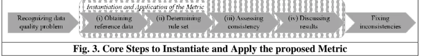
3.4 Metric Instantiation
In this subsection, we describe how to instantiate our metric. In particular, we describe how uncertain rules can be obtained and how the metric values can be calculated.
3.4.1 Obtaining Uncertain Rules
For the application of the metric, it is crucial to determine an appropriate set of uncertain rules 𝑅 and the corresponding values 𝑝(𝑟) for each uncertain rule 𝑟 ∈ 𝑅. Generally, there are different possibilities to determine this rule set. We briefly describe the following three ways: (i) Analyzing a reference dataset, (ii) Conducting a study, and (iii) Surveying experts.
Ad (i): A promising option is to use a quality assured reference dataset 𝐷𝑅 (in case such exists). This reference dataset 𝐷𝑅 needs to be representative for the data of interest in 𝐷𝐵 to allow the determination of meaningful uncertain rules. Such a reference dataset may, for example, be reliable historical data owned by the organization itself. With more and more external data being provided by recent open data initiatives, reliable publicly available data from public or scientific institutions (e.g., census data, government data, data from federal statistical offices and institutes) can be analyzed as well. The German Federal Statistical Office, for instance, offers detailed data about the population of Germany and thus for many attributes of typical master data (e.g., of customers). Further examples are traffic data as well as healthcare databases providing detailed (anonymized) data about diseases and patients. From such a reference dataset 𝐷𝑅, it is possible to determine uncertain rules for the assessment of 𝐷𝐵 directly and with a high degree of automation. In the following, we exemplarily discuss three possible ways for determining uncertain rules based on a reference dataset.
First, an association rule mining algorithm (Agrawal et al., 1993; Kotsiantis & Kanellopoulos, 2006) can be applied to 𝐷𝑅. The resulting association rules can subsequently be used as input for the metric. Applying an association rule mining algorithm in this context differs from existing works using association rules for the assessment of consistency (e.g., Alpar & Winkelsträter, 2014). In our context the rules and their confidence are not determined based on the dataset to be assessed itself, but on a reference dataset, which prevents possibly misleading results in case part of the dataset to be assessed is erroneous. Moreover, using an association rule mining algorithm in our context means that uncertain rules with a rule confidence below a chosen threshold for minimum rule confidence are not excluded.
Such rules with low confidence are beneficial for assessing consistency with the metric presented in this paper and, thus, should also be mined. This can be achieved using common association rule mining algorithms (e.g., the Apriori algorithm; Agrawal & Srikant, 1994).
Still, it is possible that for a specific data value, no association rule can be used to assess consistency because the data value is not part of an antecedent or consequent in any rule. Thus, we suggest further ways to determine or enhance a set of uncertain rules based on a reference dataset.
As a second way, we propose the use of so-called column rules, which can also be determined in an automated manner. Using column rules to assess the consistency of 𝐷𝐵 means that dependencies between different attributes are not considered. These rules consist of a tautological antecedent ⊤ (i.e., thelogical statement 𝐴 is always true) and 𝑎𝑙 = 𝜙(𝑡𝑚, 𝑎𝑙) as a consequent for all records 𝑡𝑚 in 𝐷𝑅 and attributes 𝑎𝑙 of 𝐷𝑅. This results in the rule set of the form 𝑅𝑐= {𝑟:⊤ → 𝑎𝑙 = 𝜙(𝑡𝑚, 𝑎𝑙)}, where the probability of a rule represents the relative frequency of occurrence of 𝜙(𝑡𝑚, 𝑎𝑙) in 𝐷𝑅. For example, for a record 𝑡 in 𝐷𝑅 with 𝜙(𝑡, 𝑦𝑒𝑎𝑟 𝑜𝑓 𝑏𝑖𝑟𝑡ℎ) = 1997 and 𝜙(𝑡, 𝑚𝑎𝑟𝑖𝑡𝑎𝑙 𝑠𝑡𝑎𝑡𝑢𝑠) = 𝑠𝑖𝑛𝑔𝑙𝑒, 𝑟1:⊤ → 𝑦𝑒𝑎𝑟 𝑜𝑓 𝑏𝑖𝑟𝑡ℎ = 1997 and 𝑟2:⊤ →𝑚𝑎𝑟𝑖𝑡𝑎𝑙 𝑠𝑡𝑎𝑡𝑢𝑠 = 𝑠𝑖𝑛𝑔𝑙𝑒 would be added to 𝑅𝑐.
Third, so-called row rules can also be used. Row rules are very strict with regard to their fulfillment, as all of the data values of a record need to match. These rules with tautological antecedent 𝐴 =⊤ and ⋀ (𝑎𝑎𝑙 𝑙 = 𝜙(𝑡𝑚, 𝑎𝑙)) as consequent for all 𝑡𝑚 in 𝐷𝑅 can be generated in an automated manner as well. This leads to the rule set of the form 𝑅𝑟 = {𝑟:⊤ →⋀ (𝑎𝑎𝑙 𝑙 = 𝜙(𝑡𝑚, 𝑎𝑙)) }, where the probability of a rule represents the relative frequency of occurrence of 𝑡𝑚 in 𝐷𝑅. To give an example, for a record 𝑡 in 𝐷𝑅 with 𝜙(𝑡, 𝑦𝑒𝑎𝑟 𝑜𝑓 𝑏𝑖𝑟𝑡ℎ) = 1997 and 𝜙(𝑡, 𝑚𝑎𝑟𝑖𝑡𝑎𝑙 𝑠𝑡𝑎𝑡𝑢𝑠) = 𝑠𝑖𝑛𝑔𝑙𝑒 (and no other attributes in 𝐷𝑅), the rule 𝑟3:⊤ →𝑦𝑒𝑎𝑟 𝑜𝑓 𝑏𝑖𝑟𝑡ℎ = 1997 ∧ 𝑚𝑎𝑟𝑖𝑡𝑎𝑙 𝑠𝑡𝑎𝑡𝑢𝑠 = 𝑠𝑖𝑛𝑔𝑙𝑒 would be added to 𝑅𝑟.
These three ways for obtaining uncertain rules based on a reference dataset 𝐷𝑅 were presented because of their general applicability. A large variety of further uncertain rules can be determined, for example by considering fixed attributes in the antecedent or by using different operators. Depending on 𝐷𝐵 and the specific application, any of these possibilities (or a combination of them) can be favorable as the dependencies between attributes may vary. For instance, in a context where dependencies of attributes do not have to be analyzed at all, using column rules is promising. Another example is provided in Section 4, where uncertain rules based on a reference dataset from the German Federal Statistical Office are determined. In any of these ways, the relative frequency with which 𝑟 is fulfilled in 𝐷𝑅 can be calculated and used as 𝑝(𝑟). Thereby, based on 𝐷𝑅 both rules and corresponding
probabilities of fulfillment can be determined with a high degree of automation. This allows a use of multiple rule sets to focus on different aspects of the data to be assessed or to analyze the specific reasons for inconsistencies in the data (cf. Section 4).
When using a reference dataset 𝐷𝑅 for determining rules, the number
|𝑓𝑢𝑙𝑓𝑖𝑙𝑙𝑖𝑛𝑔 𝑟𝑒𝑐𝑜𝑟𝑑𝑠(𝐷𝑅, 𝐴 ∧ 𝐶)| of records in 𝐷𝑅 fulfilling a rule needs to be sufficiently large to ensure reliable metric values with respect to this rule. To be more precise, the statistical significance of 𝑝(𝑟) needs to be assured. If an association rule mining algorithm is used, a suitable minimum support can be fixed to exclude rules based on a non-significant proportion of records. In any case, a statistical test can be applied in order to determine the minimal number of records required such that a rule has a significant explanatory power (cf. Section 4). Moreover, to provide a statistically reliable basis and to circumvent the aforementioned issue, rules can be aggregated (e.g., by using a disjunction). In this way, robust estimations of 𝑝(𝑟) can be obtained, allowing the determination of reliable metric values.
Ad (ii): If neither internal nor external reference data is available, conducting a study is a further possibility. For example, if a customer database is to be assessed, a random sample of the customers can be drawn and surveyed. The survey results can be used to determine appropriate uncertain rules by analyzing the customers’ statements. Moreover, the corresponding values of 𝑝(𝑟) for each rule 𝑟 can be obtained by analyzing how many of the surveyed customers fulfill the rule. Thus, the input parameters for the metric are provided. As a result of the survey, one obtains quality assured data of the surveyed customers and can also assess the consistency of the data of customers not part of the survey.
Ad (iii): Another possibility is to use an expert-based approach (similar to Mezzanzanica et al., 2012;
Baker & Olaleye, 2013; Meyer & Booker, 2001). Here, the idea is to survey qualified individuals. For rules in a customer database of an insurer taking into the account the attributes number of insurance relationships, insurance group and fee paid, insurance experts could be surveyed. Another example concerns very rare events such as insurance exclusions without reimbursement, for which not enough (reference) data is available. The experts can assess which rules are suitable to describe the expected structure of the considered data values and can specify the respective values of 𝑝(𝑟) for each rule.
3.4.2 Calculating the Metric Values
Based on a set of uncertain rules 𝑅 with values 𝑝(𝑟) for each 𝑟 ∈ 𝑅, the metric values can be calculated in an automated manner. The values |𝑓𝑢𝑙𝑓𝑖𝑙𝑙𝑖𝑛𝑔 𝑟𝑒𝑐𝑜𝑟𝑑𝑠(𝐷𝐵, 𝐴)| and |𝑓𝑢𝑙𝑓𝑖𝑙𝑙𝑖𝑛𝑔 𝑟𝑒𝑐𝑜𝑟𝑑𝑠(𝐷𝐵, 𝐴 ∧ 𝐶)| can be determined efficiently via simple database queries. In addition, based on the value of 𝑝(𝑟), the corresponding binomial distribution can be instantiated. Then, the (two-sided) p-value with regard to |𝑓𝑢𝑙𝑓𝑖𝑙𝑙𝑖𝑛𝑔 𝑟𝑒𝑐𝑜𝑟𝑑𝑠(𝐷𝐵, 𝐴 ∧ 𝐶)| can be calculated in order to obtain the metric values.
In the literature, several different approaches to calculate the two-sided p-value have been proposed (Dunne, Pawitan, & Doody, 1996). These include doubling the one-sided p-value and clipping to one, summing up the probabilities less than or equal to the probability of the observed result, and more elaborate ways. In practical applications, for non-symmetric distributions, the approaches to calculate the two-sided p-value may lead to slightly different results. However, the larger the sample size (in our case |𝑓𝑢𝑙𝑓𝑖𝑙𝑙𝑖𝑛𝑔 𝑟𝑒𝑐𝑜𝑟𝑑𝑠(𝐷𝐵, 𝐴)|), the smaller the differences between the results of the different approaches are. This is due to the fact that for 𝑝(𝑟) ∈ (0; 1), the binomial distribution converges to the (symmetric) normal distribution (de Moivre-Laplace theorem).
4 Evaluation
In this section we evaluate (E1) the practical applicability as well as (E2) the effectiveness (Prat, Comyn- Wattiau, & Akoka, 2015) of our metric for consistency in a real-world setting. First, we discuss the reasons for selecting the case of a German insurer and describe the assessed customer dataset. Then, we show how the metric could be instantiated for this case. Subsequently, we present and discuss the results of the application. Finally, we compare the results with those of existing metrics for consistency.
4.1 Case Selection and Dataset
The relevance of managing customer data at a high data quality level is well acknowledged (cf. e.g., Even, Shankaranarayanan, & Berger, 2010; Heinrich & Klier, 2015b). The metric was applied in cooperation with one of the major providers of life insurances in Germany. High data quality of customer master data is critical for the insurer and plays a particularly important role in the context of customer management. However, the staff of the insurer suspected data quality issues due to negative customer feedback (e.g., in the context of product campaigns). Customers claimed to have a marital status
different from the focused target group of campaigns. Thus, they either were not interested in the product offerings or were not even eligible to participate. To analyze these issues, we aimed to assess the consistency of the customers’ marital status depending on their age.
This setting seemed particularly suitable for showing the applicability and effectiveness of our metric for the following reasons: First, the marital status of a customer is a crucial attribute for the insurer, because insurance tariffs and payouts often vary depending on marital status. Indeed, for example a customer whose marital status is erroneously stored as widowed may receive unwarranted life insurance payouts. Additionally, the marital status also significantly influences product offerings, as customers with different marital statuses tend to have varying insurance needs. In fact, as mentioned above, customers may even only be eligible for a particular insurance if they have a specific marital status. Second, interpretable metric values are of particular importance in this setting, for instance to facilitate the aforementioned product offerings. Third, using traditional rules which are “true by definition” is not promising here as except for children, who are always single, no marital status is definite or impossible for customers. For example, a 60-year-old customer may be single, married, divorced, widowed, etc., each with specific probability.
To conduct the analyses described above, the insurer provided us with a subset of its customer database. The analyzed dataset contains five attributes storing data about customers of the insurer born from 1922 onwards and represents the state of the customer data from 2016. The subset consists of 2,427 records which had a value for both the attribute marital status and the attribute date of birth. Each record represents a specific customer of the insurer. The marital status of the customers was stored as a numerical value representing the different statuses single, married, divorced, widowed, cohabiting, separated and civil partnership. As the marital statuses cohabiting and separated are not recognized by German law (Coordination Unit for IT Standards, 2014), we matched these statuses to the respective official statuses single and married. The date of birth was stored in a standard date format. On this basis, customers’ age could easily be calculated and stored as an additional attribute age. Moreover, an attribute gender was available both in the customer dataset as well as in the data used for the instantiation of the metric (cf. following subsection). As gender may have a significant impact on marital status as well, we also included this attribute in our analysis. Each of the 2,427 records contained a value for
gender, classifying the respective customer as either male or female.
4.2 Instantiation of the Metric for Consistency
In Section 3.4.1, we described possibilities to obtain a set of uncertain rules for the instantiation of our metric. In our setting, we were able to use publicly available data from the German Federal Statistical Office as a reference dataset and thus chose option (i). The German Federal Statistical Office provides aggregated data regarding the number of inhabitants of Germany having a specific marital status. We used the most recent data available, which is based on census data from 2011 and was published in 2014 (German Federal Statistical Office, 2014). The data is broken down by age (in years) as well as gender and includes all Germans regardless of their date of birth, containing in particular the data of the insurer’s customers. Overall, the data from the German Federal Statistical Office seems to be an appropriate reference dataset for our setting and could be used to determine meaningful uncertain rules and the probabilities 𝑝(𝑟) for each rule 𝑟.
As it was our aim to examine consistency of the marital status of customers depending on their age and gender, both attributes age and gender were part of the antecedent of the rules while the attribute marital status was contained in the consequent. To determine a rule set, we proceeded as follows: First, for each marital status m, each gender g and each possible value of age a ∈ ℕ, we specified rules of the following form:
𝑟𝑚,𝑔𝑎 : (𝑎𝑔𝑒 = 𝑎) ∧ (𝑔𝑒𝑛𝑑𝑒𝑟 = 𝑔) → 𝑚𝑎𝑟𝑖𝑡𝑎𝑙 𝑠𝑡𝑎𝑡𝑢𝑠 = 𝑚 (7) Second, we calculated the probabilities 𝑝(𝑟𝑚,𝑔𝑎 ) based on the data from the German Federal Statistical Office. Third, starting at an age of 0 years, we systematically aggregated these rules to rules of the form:
(𝑎𝑔𝑒 ≥ 𝑎1) ∧ (𝑎𝑔𝑒 < 𝑎2) ∧ (𝑔𝑒𝑛𝑑𝑒𝑟 = 𝑔) → 𝑚𝑎𝑟𝑖𝑡𝑎𝑙 𝑠𝑡𝑎𝑡𝑢𝑠 = 𝑚 (8) Here, 𝑎1, 𝑎2∈ ℕ (with 𝑎1 < 𝑎2) specify an age group. The aggregation of the rules 𝑟𝑚,𝑔𝑎 was performed to increase the number of records each rule was relevant for. However, age groups also have to be homogeneous and thus, the differences in probabilities of rule fulfillment within an age group were required to not exceed a specific threshold. More precisely, for a given value of 𝑎1, the value 𝑎2 was determined to be the maximum of all values 𝑗 ∈ ℕ for which |𝑝(𝑟𝑚,𝑔𝑗 ) − 𝑝(𝑟𝑚,𝑔𝑘 )| ≤ 0.1 held for all
𝑎1≤ 𝑘 ≤ 𝑗. In this way the following rule 𝑟̃ for single men between 42 and 49 was obtained:
𝑟̃: (𝑎𝑔𝑒 ≥ 42) ∧ (𝑎𝑔𝑒 < 50) ∧ (𝑔𝑒𝑛𝑑𝑒𝑟 = 𝑚𝑎𝑙𝑒) → 𝑚𝑎𝑟𝑖𝑡𝑎𝑙 𝑠𝑡𝑎𝑡𝑢𝑠 = 𝑠𝑖𝑛𝑔𝑙𝑒 (9)
Afterwards, for each rule 𝑟 ∈ 𝑅 the probabilities 𝑝(𝑟) were calculated based on the data from the German Federal Statistical Office. For example, as approximately 26.4% of men between 42 and 49 are single according to the German Federal Statistical Office, this resulted in 𝑝(𝑟̃)=0.264. Moreover, a statistical test to the significance level of 0.05 was applied to ensure that each rule is based on a statistically significant number of relevant records in both the reference dataset and the customer dataset.
Rules not fulfilling the test were excluded from further analysis to guarantee reliable metric results. This way, 37 different rules and corresponding probabilities were determined.
Each customer record of the insurer belonged to one of the age groups and had the value male or female for the attribute gender and the value single, married, divorced, widowed or civil partnership for the attribute marital status as represented by our rule set. Accordingly, a metric value could be determined for the value of the attribute marital status of each of these records. For instance, to assess the consistency of the marital status single of a 46-year-old male customer 𝑡, 𝑟̃ was used. The calculation of the metric value by means of Definition (6) yielded a consistency of 0.888:
𝑄𝐶𝑜𝑛𝑠(𝜙(𝑡, 𝑠𝑖𝑛𝑔𝑙𝑒), 𝑟̃) = 𝑝-𝑣𝑎𝑙𝑢𝑒(𝑋(𝑟̃)~𝐵(57,0.264), 14) = 0.888 (10)
To calculate the two-sided p-value, we doubled the one-sided and clipped to one (Dunne et al., 1996).
4.3 Application of the Metric for Consistency and Results
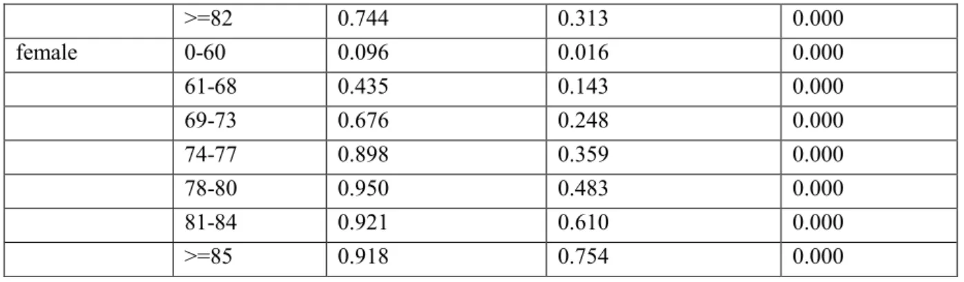
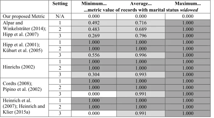
Having instantiated the metric, we applied the metric to the 2,427 customer records by means of a Java implementation. The results for the marital status widowed seemed particularly interesting and alarming.
Indeed, in contrast to the other marital statuses, analyses for this marital status revealed that the metric values were very low across all customer records. In fact, for the 1,160 records with a marital status of widowed, the metric value was always below 0.001 (cf. Table 2).
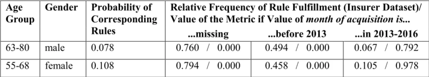
Gender Age Group Relative Frequency of Rule Fulfillment (Insurer Dataset)
Probability of Corresponding Rule (Statistical Office)
Value of the Metric for Consistency
male 0-74 0.139 0.012 0.000
75-81 0.713 0.132 0.000