Randomly Pinned Systems: Interfaces and Luttinger Liquids

Interfaces and Luttinger Liquids

Inaugural-Dissertation zur

Erlangung des Doktorgrades

der Mathematisch-Naturwissenschaftlichen Fakult¨ at der Universit¨ at zu K¨oln

vorgelegt von Friedmar Sch¨ utze

aus Leipzig

K¨oln, 2010

Tag der m¨ undlichen Pr¨ ufung: 15. Oktober 2010

Contents

Introduction 1

1 AC-driven interfaces in random media 3

1.1 Introduction . . . . 3

1.2 The model . . . . 5

1.2.1 The equation of motion . . . . 5

1.2.2 The mean-field equation of motion . . . . 6

1.3 Mean field theory . . . . 7

1.3.1 The zero frequency limit . . . . 8

1.3.2 Finite Frequencies . . . . 18

1.4 Perturbation theory . . . . 25

1.4.1 The diagrammatic expansion . . . . 26

1.4.2 The failure of perturbation theory for D ≤ 4 . . . . 29

1.4.3 Interfaces subject to a constant driving force . . . . 31

1.5 Mean field perturbation theory . . . . 33

1.5.1 The diagrammatic expansion . . . . 33

1.5.2 Regularity of the perturbative series . . . . 35

1.5.3 Validity of perturbation theory . . . . 35

1.5.4 Perturbative harmonic expansion . . . . 36

1.6 Summary and Conclusions . . . . 40

2 The effect of electroelastic coupling on ferroelectric domain walls 41 2.1 Introduction . . . . 41

2.2 Electrostrictive coupling . . . . 42

2.2.1 The model . . . . 43

2.2.2 The effective Hamiltonian . . . . 44

2.2.3 The interface Hamiltonian . . . . 45

2.3 A simple model for KDP-type ferroelectrics . . . . 48

2.3.1 The model . . . . 48

2.3.2 The interface Hamiltonian in harmonic approximation . . . . 50

2.3.3 Domain wall roughness in the presence of random field disorder . . . . . 52

2.3.4 Needle domains . . . . 53

3 Luttinger liquids with disorder 55

3.1 Introduction . . . . 55

3.2 The model . . . . 57

3.2.1 The disorder term . . . . 57

3.2.2 The replica action . . . . 60

3.3 Absence of the Mott Glass phase . . . . 62

3.3.1 Generalised rigidities . . . . 62

3.3.2 The ac conductivity . . . . 63

3.3.3 Fixed points and phases . . . . 64

3.3.4 The phase diagram . . . . 66

3.3.5 Concluding remarks . . . . 68

3.4 The replica instanton approach . . . . 68

3.4.1 The Euler-Lagrange equations . . . . 69

3.4.2 Solution of the Euler-Lagrange equations . . . . 70

3.4.3 A toy model . . . . 76

A Appendices to chapter 1 83 A.1 Numerics . . . . 83

A.2 Generation of disorder forces with a cusped correlator . . . . 85

A.3 Derivation of the potential energy balance . . . . 86

A.4 The functional integral approach . . . . 87

A.5 The regularity of all perturbative orders in case D > 4 . . . . 89

A.6 Analysis of the bush graphs . . . . 94

A.7 The width of ac-driven interfaces . . . . 96

A.8 Regularity of the mean-field perturbation expansion . . . . 98

B Appendices to chapter 2 101 B.1 Interface Hamiltonian for the φ ⁴ model . . . 101

B.2 The harmonic approximation . . . 102

B.3 Derivation of H ee . . . 103

Bibliography 105

Danksagungen 113

Abstract 115

Zusammenfassung 117

Erkl¨ arung 119

Lebenslauf 121

Introduction

Over many decades, pioneering work in classical statistical mechanics has bred a canonical formalism to describe macroscopic systems in equilibrium, starting from microscopic models.

The basic concept consists in averaging over microscopic degrees of freedom, that are irrele- vant for macroscopic properties. These ideas have later been adopted to include also systems of many quantum particles. Their quantum nature becomes important at low temperatures.

Nowadays, the application arena of statistical mechanics includes not only the evident fields of solid state physics, atomic physics, optics and chemistry but also covers the realms of cosmol- ogy as well as biology. Recent years have witnessed that the scope of statistical mechanics even successfully strives beyond the frontiers of pure natural sciences towards theoretical computer science, coding theory and quantitative finance.

The present challenges of statistical mechanics are mainly provided by systems out of equilibrium, noise induced behaviour and phenomena arising from the presence of disorder. In these areas, even classical physics is far from being exhaustively explained. The significance of an understanding of disordered systems can thereby hardly be overestimated. On the one hand, impurities and lattice defects are ubiquitous in everyday life materials, which suggests the technological quest for a quantitative description of possible deviations from results obtained using models for pure systems. On the other hand, the presence of disorder also has a major impact on the underlying physics. For instance, arbitrarily weak amounts of disorder increase the lower critical dimension of the Ising model [1] and drive non-interacting electronic systems from metallic to insulating behaviour in less than or equal to two dimensions [2]. Remarkably, some exciting phenomena, like the integer quantum Hall effect, even require the presence of disorder to appear.

A major difficulty with the study of random systems consists in the, frequently rather hidden, collapse of useful mathematical tools. A prominent illustrative example is the failure of dimensional reduction in connection with the random field Ising model [1], which has led to a long controversy about the lower critical dimension of this system. The idea of dimensional reduction is based on a conclusion from perturbation theory, that a d-dimensional random field system obeys the same critical behaviour like its pure counterpart in d − 2 dimensions [3].

It relies, however, on the incorrect assumption that perturbation theory is applicable. This will be discussed in more detail in chapter 1. It demonstrates, that for disordered systems, the art is to develop simple arguments which, fortunately, often turn out to be astonishingly robust. An example for such a stable but simple tool is the Imry-Ma argument [4].

In this thesis we treat two different kinds of systems exposed to disorder. In the first

two chapters, we are dealing with elastic interfaces and in the last part, we take a look at

one-dimensional fermionic quantum systems, so called Luttinger liquids. It is important to distinguish between two types of disorder.

(1) On the one hand, disorder may arise from isolated strong impurities, which serve as single pinning centres or scatterers.

For elastic interfaces, the pinning at single strong impurities sets a length scale, which is given by the typical distance l _imp between the impurities. This kind of pinning is of course only possible, if l imp is large enough as compared to the thickness of the interface.

In Luttinger liquids, the effect of an isolated strong impurity is relevant in case of repulsive interaction (K < 1, for the meaning of K cf. chapter 3) [5].

(2) On the other hand, disorder can also be created by a finite density of weak impurities which act collectively. This is the so called Gaussian disorder.

Applied to elastic interfaces, where the disorder competes with the elasticity, the effect of many weak impurities has to accumulate to be able to oppose the elastic forces. Thus, in sufficiently low dimensions, the interplay of randomness and elasticity introduces a new length scale, called the Larkin length, above which disorder is strong enough to overcome elasticity. Whence beyond the Larkin length the static configuration of the system is mainly determined by the disorder and the interface is pinned at the fluctuations of the impurity density. In high dimensions, the elastic term dominates on all length scales and the interface is not pinned by weak disorder.

In Luttinger liquids the critical K below which the disorder is relevant is now shifted to K c = 3/2 [6], whence also for weak attractive interaction disorder leads to localisation.

In this thesis, the focus is on quenched disorder of the second type, i.e. weak Gaussian disorder.

In the remainder of this introduction, we provide an outline of this thesis. Three different topics are considered, each of which is assigned an own chapter. All chapters should be self-contained to the greatest possible extent and can be read independently. Moreover, a comprehensive introduction to each topic is provided at the beginning of every chapter, so that in the following we describe only briefly the subjects and how this thesis is organised.

The topic of chapter 1 concerns interfaces in disordered systems, driven by an external force. Emphasis is put on the case of an ac-driving, for which we analyse the mean-field theory and study the perturbation expansion. In chapter 2, we consider a special case of elastic interfaces, namely domain walls in ferroelectric materials. The work in this part concentrates on the statics. We examine the effect of electroelastic coupling on the domain wall stiffness and use an Imry-Ma argument to predict the roughness in the presence of random-field disorder.

In chapter 3, we leave the realm of purely classical physics and consider one-dimensional

fermionic quantum liquids. First, we study the effect of randomness on the Mott state and

dismiss the idea of a Mott glass phase, the existence of which has been hypothesised in recent

publications. Then, we discuss the replica trick applied to the quantitative analysis of the

conductivity in disordered one-dimensional electronic systems.

AC-driven interfaces in random media

1.1 Introduction

The overdamped motion of an elastic manifold in a disordered environment, subject to an external driving force, is a key problem in the field of non-equilibrium statistical mechanics, that has attracted much attention for now more than two decades [7, 8]. Examples of phys- ical systems that can be described by such models include interfaces, e.g. domain walls in disordered ferroic systems [9] or interfaces between immiscible fluids that are pushed through porous media [10, 11], as well as vortex lines in impure superconductors [12, 13, 14], dislocation lines in a solid [15] or driven charge density waves [16].

The importance of the effect of disorder on the motion of elastic systems arises in different contexts. In type-II superconductors, flux lines enclose normal conducting electrons in their core. The motion of a flux line thus ultimately causes energy dissipation. The presence of disorder leads to a pinning of the flux lines at attractive impurities and hence prevents their motion, so superconductivity is sustained. Other examples are the hardening of steel through pinning of dislocation lines by randomly distributed carbon atoms in the material, and the suppression of domain wall motion in ferroic memories.

Quite generally, elastic systems in random media exhibit a depinning threshold [17]. At zero temperature and below a certain critical driving force h p , the system is pinned and remains at rest. Only if the force h exceeds h _p , the system moves with a finite velocity. Close to depinning, this velocity obeys a power-law dependence on the distance to the threshold, v ∼ (h − h _p ) ^β . For finite temperatures, creep motion is present also below the critical force.

The depinning phenomenon at zero temperature shares many features with continuous

phase transitions in equilibrium. In this analogy, v can be considered to play the role of an

order parameter and one expects critical behaviour close to depinning. It is, however, highly

non-trivial to obtain a quantitative understanding of this dynamic critical phenomenon. After

a long controversy about the lower critical dimension d _l of the random field Ising model,

which has been predicted to be d _l = 3 by dimensional reduction and d _l = 2 by Imry-Ma

domain wall arguments [4], it has been pointed out by D.S. Fisher [1], that disordered elastic

systems have to be studied within a functional renormalization group (FRG) approach. The latter is necessary because the disorder force correlator develops a cusp singularity in the course of the FRG flow. Using FRG methods, the critical behaviour of finite dimensional interfaces [18, 19, 20, 21], charge density waves [22] and contact lines [23] has been worked out. These FRG studies have even been extended to take into account higher loop corrections [24, 25, 26]. The influence of finite temperatures has been studied as well, both, close to depinning [27, 28, 29, 30] and in the creep regime [28, 31, 32].

Beyond the problem of constant forces, the dynamics of ac-driven interfaces in random media recently became a subject of increasing prominence. Of special experimental interest is the ac susceptibility of ferroic systems [33, 34] which gets a considerable contribution from the domain wall motion [35, 36]. A phenomenological understanding of different regimes has been reported in Ref. [37], where the concept of waiting time distributions has been used.

Moreover, an extension of the FRG flow equations from the problem with a constant driving force, combined with a scaling analysis has been used to work out the main characteristics of the velocity hysteresis loop [38]. In the limit of small frequencies, scaling behaviour has been found and the exponents of the remanent velocity at depinning as a function of frequency that have been determined for all dimensions D < 4 agree very well with numerical results. Further study of ac-driven elastic systems has been devoted to vortex lattices [39] and structural defects in liquid crystals [40].

Many questions related to ac-driven interfaces remain open. The mean-field equation of motion is not yet analysed, and a quantitative description of the velocity hysteresis has so far not been achieved. In this chapter, we are going to address some of the unsolved problems in the field. Our results are published in Refs. [41, 42]. A description of our work and how it embeds in the framwork of previous study, is given at the beginning of each section. Here, we briefly describe how the present chapter is organised.

In the following section, we introduce the model equation of motion, discuss some impor- tant scales and derive the associated mean field theory.

In section 1.3, we study the mean field problem of driven interfaces in random media, where we distinguish between a smooth force correlator and a force correlator that has a cusp singularity at the origin. We start with an analysis of the problem with constant driving forces for which we discuss the motion close to depinning and derive the critical exponents. Then, we go over to consider ac-driven interfaces. Our main focus lies on the critical dynamics for small driving frequencies, which we study by analytical and numerical methods. We find power-law scaling for the velocity as well as the hysteresis loop area.

In section 1.4, we aim at going beyond mean-field theory and investigate the perturbative

expansion of the equation of motion for ac-driven domain walls. After analysing the first

non-vanishing order, we derive the diagrammatic expansion to account for higher orders. This

can be used to argue, that perturbation theory works for D > 4. We will, however, see that in

all physically interesting dimensionalities D ≤ 4, perturbation theory is no longer useful. The

failure of perturbation theory for D ≤ 4 is analysed and explained. The well-known use of

perturbation theory for estimates of the velocity of domain walls driven by a constant force,

far in the sliding regime, does not contradict our statements for the ac-driving. We are going

to take a look at this as well. The technically involved and more mathematical treatments are

taken out of the main text and given in the appendices.

Formally corresponding to infinite dimensionality, mean-field theory admits a regular per- turbation expansion. In section 1.5, we explore the perturbative series and numerically show, that it agrees very well with the solution to the full mean field equation. We prove, that the perturbative corrections are regular, i.e. they remain bounded in all orders. The bulk part of this inductive proof, the induction step, is outsourced to appendix A.8. Based on a numerical analysis, we conjecture a power-law scaling of the decay constants for the Fourier coefficients of the mean velocity with the strength of the driving force.

1.2 The model

1.2.1 The equation of motion

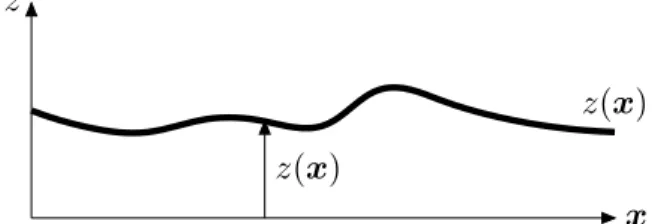
Our analysis models interfaces and domain walls that are thin such that they can be described by elastic D-dimensional manifolds, embedded in a D + 1-dimensional space. The manifold

z

x z( x )

z( x )

Fig. 1.1: Illustration of an elastic manifold, parametrised by a D-dimensional vector x x x. Overhangs are not allowed.

itself is parametrised by a D-dimensional set x x x of coordinates and its position in space is given by z(x x x, t). We confine ourselves to the study of the zero-temperature case, i.e. we do not take thermal noise into account. Moreover, our model assumes small gradients and does not allow for overhangs. We expose the interface to a periodic driving force

h(t) = h · cos ωt. (1.1)

Then, the overdamped dynamics of elastic interfaces can be described by the equation of motion

γ

¹ ∂ _t z(x x x, t) = Γ ∇ x ² x x z + h(t) + u · g(x x x, z), (1.2) which has already been introduced in earlier works [43, 44, 45]. In Eq. (1.2), Γ and γ are the stiffness and the inverse mobility of the domain wall. For simplicity, we set γ = 1 in the following. The function g(x x x, z) describes the quenched disorder, taken to be Gaußian with the correlators given by

h g(x x x, z) i = 0 (1.3)

g(x x x, z)g(x x x

, z

)

= δ ^D (x x x − x x x

)∆(z − z

), (1.4)

where h . . . i denotes the average over disorder. The disorder correlator in z-direction is taken

symmetric around 0 and decays exponentially on a length scale ℓ. Further, we demand ∆(0) =

1, as the strength of the disorder shall be measured by u. To be definite, we choose

∆(z − z

) = exp

"

−

z − z

ℓ

2 #

(1.5) in case we need a precise formula. This choice corresponds to the case of an elastic interface exposed to random field disorder [20]. Throughout the whole chapter we assume weak disorder.

This means, that pinning forces are weak and the interface is pinned at the fluctuations of the impurity concentration, and not at single pinning centres. A more precise definition can be found e.g. in Ref. [46]. For weak disorder, the random forces have to accumulate to overcome the elasticity. On small length scales, elastic forces dominate and the interface is essentially flat. By comparing the elastic and the disorder term in (1.2) one can estimate the length scale L _p , called the Larkin length, at which the two competing effects are of the same order. The result is

L _p = Γℓ

u

. (1.6)

Thus, the elastic term dominates on all length scales for D > 4. Finally, we have to specify the initial configuration for the equation of motion (1.2), which we choose to be a flat wall z(x x x, t = 0) ≡ 0.

1.2.2 The mean-field equation of motion

To obtain the mean field equation corresponding to our original equation of motion (1.2), we have to replace the elastic term by a uniform long-range coupling (cf. e.g. [47]). To do this, we formulate the model (1.2) on a lattice in x x x-direction, i.e. the coordinates that parameterise the interface itself are discretised. The lattice Laplacian reads

∇ ² x x x z(x x x _i ) =

D

X

d=1

z(x x x _i + aeee _d ) + z(x x x _i − aeee _d ) − 2z(x x x _i )

a ² =

D

X

d=1 N

X

j

=1

J _ij

z(x x x _j

) − z(x x x _i )

, (1.7) J ij

= 1

a ²

δ j

+1,i + δ j

1,i

, (1.8)

where a denotes the lattice constant. To get the mean field theory, J _ij is replaced by a uniform coupling but such that the sum over all couplings P

j J _ij remains the same. Hence, we choose J _ij ^MF = 1

a ² N . (1.9)

Now, the disorder has to be discretised as well, which is achieved if we replace the delta function in the correlator (1.4) by δ ^D (x x x i − x x x j ) → δ ij a

^D/2 (cf. Ref. [44]). The resulting equation of motion should be independent of x x x, just the lattice constant a and the dimension enter because the disorder scales with a factor a

^D/2 . Further, we replace the spatial average by the ensemble average with respect to the probability distribution of the disorder P [g]

X

i

z(x x x _i , t) = Z

Dg(z) P [g(z)]z(t) ≡ h z(t) i , (1.10)

which is justified in the thermodynamic limit, where the spatial average does not fluctuate.

Finally, for the mean-field equation of motion, we obtain

∂ _t z = c · [ h z i − z] + h(t) + η · g(z), (1.11) where c = Γ/a ² and η = u/a ^D/2 . The disorder remains Gaußian with

h g(z) i = 0 (1.12)

g(z)g(z

)

= ∆(z − z

). (1.13)

As before, ∆(z) is a function that decays to zero on a length scale ℓ and obeys ∆(0) = 1. For the mean field equation of motion we are going to consider two different types of correlators. We distinguish between a correlator that is smooth and a correlator that shows a cusp singularity at the origin. As has been mentioned in the introduction, a cusp singularity in the correlator emerges as a fixed point solution of the functional renormalization group (FRG) flow in 4 − ǫ dimensions and describes the effective randomness on scales larger than the Larkin length.

This leads to the existence of a depinning threshold in all dimensions d < 4. Of course, in the framework of the mean field approximation an FRG study is senseless and a correlator with a cusp singularity has to be included manually.

The physical picture of the mean field equation of motion is that of a system of distinct particles, moving in certain realisations of the disorder. All of them are harmonically coupled to their common mean, i.e. the elastic coupling between neighbouring wall segments Γ ∇ ² x x x z is now replaced by a uniform coupling c · [ h z i − z] to the disorder averaged position h z i , which in turn is determined self-consistently by the single realisations.

Apart from the correlation length ℓ of the disorder, there is another important length scale in the system. In the absence of any driving force (i.e. h = 0), we can easily determine the mean deviation of the coordinate z of a special realisation from the disorder averaged position h z i . For h = 0 we have ˙ z = 0 and (1.11) straightforwardly leads to

( h z i − z) ²

≃ η ²

c ² . (1.14)

So, η/c measures the order of the average distance from the common mean.

In what follows, the disorder averaged velocity v = h z ˙ i will be denoted by the symbol v.

1.3 Mean field theory

A useful tool to achieve first insight in complicated physical problems is the mean field ap- proximation. Before embarking on our mean-field treatment of driven domain walls, we briefly highlight the historical development of this field.

More than two decades ago, in a seminal work, D.S. Fisher has studied the depinning of

charge density waves (CDW) from randomly distributed pinning centres [48, 47] by an external

field h. He showed that the depinning transition is a dynamical critical phenomenon where

the velocity close to the depinning threshold h _p plays the role of an order parameter exhibiting

a power law behaviour v ∼ (h − h _p ) ^β . Within the mean-field approach, developed in [48, 47], the exponent β was found to be β = 3/2.

The mean field theory for driven interfaces in disordered systems has first been considered by Koplik and Levine [45] within the framework of perturbation theory. They found that the interface either follows a solution which moves with constant velocity or it remains pinned.

They were, however, not able to extend their findings to the problem of spatially extended interfaces, because their perturbative approach lacks the necessary FRG analysis.

In a subsequent work, Leschhorn studied the mean field theory for domain walls in a model which treats the disorder in a simplified manner [49]. He considered a discretised lattice system and allowed the random force field to take values out of three possibilities only: − 1, 0 or +1.

For his model, he also found pinned and sliding solutions and determined the velocity exponent as β = 1, which is the same as for CDWs when the disorder force has discontinuous jumps [22].

Vannimenus and Derrida [50] simplified the Leschhorn model even further and were able to derive an exact solution. The basic simplification of their model concerns the assumption of unit moves. This means, that per unit time step a segment of the interface either remains at rest, if the total force is smaller or equal to zero. Otherwise, it moves exactly one step forward, independent of the magnitude of the force. Though this assumption admits an exact solution, the restriction to unit moves entails a non-uniform periodic behaviour of the mean velocity close to the threshold. The time averaged velocity (over one period) has then a different exponent β = 1/2.

In the following, we present our work on the mean field theory for driven interfaces, modeled by Eq. (1.11). If not otherwise stated, throughout this section we measure z in units of ℓ and t in units of ℓ/η, such that ℓ = η = 1.

1.3.1 The zero frequency limit

In this subsection, we consider a special case of the equation of motion (1.11), for which the driving force is constant in time. The equation of motion reads

∂z

∂t = c ( h z i − z) + h + g(z). (1.15) At sufficiently large driving force h, the average particle position h z i will move with constant velocity v ≥ 0. In this case, Eq. (1.15) can be written as

∂ _t z = c (vt − z) + h + g(z) = g(z) − [c (z − vt) + h]. (1.16)

In the following we will consider the case where the velocity is sufficiently small v ≪ h. The

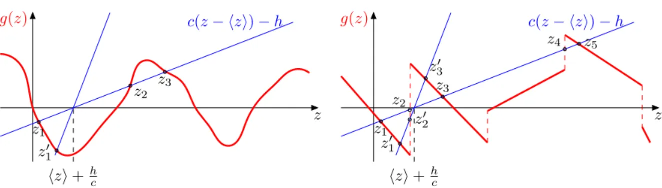
positions where ∂ _t z = 0 follow from the intersection of g(z) with the straight line c(z − vt) − h

which moves to the right with velocity v (cf. Fig. 1.2). For sufficiently small c and smooth

g(z) there are in general 2n + 1 intersections which we denote by z ₁ < z ₂ < z ₃ < . . .. For

z < z ₂ , z is driven towards z ₁ , for z ₂ < z < z ₄ it is driven towards z ₃ etc. If the particle starts

with an arbitrary initial value, it will first develop towards the closest stable fixed point of

(1.16), where the particle velocity is small. Let us assume this is z ₁ . The force free point z ₁

will then change according to z ₁ (t) = vt + h/c + g(z ₁ )/c. Eventually, the intersection point

c(z − hzi) − h

z

z

z

z

z

hzi +

g(z)

Fig. 1.2: Plot of the left and the right hand side of equation (1.20) for random forces with a smooth correlator. For small c there are several intersec- tion points, for small values of c there is only one solution.

c(z − hzi) − h

z

z

z

z

z

z

z

z

z

hzi +

g(z)

Fig. 1.3: Plot of the left and the right hand side of equation (1.20) for random forces accociated to a scalloped potential, which shows a cusp singularity in the correlator. Random force realisations with a jump close to the origin yield more than one solution even for very small values of c.

z ₁ (t) merges with z ₂ (t) and then disappears. In this case z(t) will grow sufficiently fast until it reaches z 3 (t) and the process repeats if we replace z n → z n

2 . Thus, the motion of the particle is jerky: periods of slow motion with velocity v are intermitted by fast periods where the particle is driven towards a new stable fixed point. Below, we will analyse this process in detail.

The general picture

A first overview results from considering some limiting cases.

(i) For large but finite c we can apply perturbation theory. Decomposing z(t) = vt + ζ (t), to lowest non-trivial order one obtains for the mean velocity (the derivation is analogous to the perturbation theory derived in Sec. 1.5)

v = h + Z

0

dt e

^ct ∆

(vt) . (1.17)

The depinning threshold h _p,

for h ≶ 0 follows from taking the limit v → ± 0, h → ± h _p ± 0 h _p,

≡ − lim

ε

0 c

¹ ∆

( ± ε). (1.18)

Thus, the force correlator has to have a cusp singularity to produce a finite threshold. If there is no cusp, perturbation theory in c

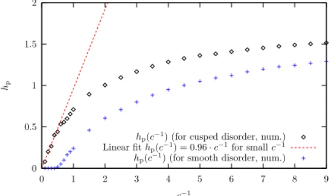
¹ signals the absence of a depinning threshold. This argument applies however only to the region where perturbation theory is applicable, i.e. for c ≫ 1. This perturbative result is in accordance with our numerical analysis, as is shown in Fig. 1.4.

As has been mentioned in the introduction, a cusp singularity in the correlator emerges as a

fixed point solution of the functional renormalization group (FRG) flow in 4 − ǫ dimensions and

describes the effective randomness on scales larger than the Larkin length. This leads to the

existence of a depinning threshold in all dimensions D < 4. Of course, in the framework of the

mean field approximation an FRG study is senseless and a correlator with a cusp singularity has to be included manually. Nevertheless, as we already see here, in many aspects the assumption of a correlator with a cusp gives different results compared to a smooth correlator.

0 0.5 1 1.5 2

0 1 2 3 4 5 6 7 8 9

hp

c⁻¹

h_p(c⁻¹) (for cusped disorder, num.) Linear fith_p(c⁻¹) = 0.96·c⁻¹for smallc⁻¹ h_p(c⁻¹) (for smooth disorder, num.)

Fig. 1.4: Depinning threshold as a function of c

in the case of a dc-drive, ω = 0. For the case of a cusp-correlator of the random forces (diamonds) the depinning threshold remains finite as long c

is finite. For a smooth correlator (crosses) the threshold vanishes for small c

as expected from perturbation theory.

(ii) Finally, we consider the case c ≪ 1. For c = 0 the equation of motion (1.15) can be integrated

Z _z

0

dz

h + g(z

) = t. (1.19)

To calculate the integral we assume that h > 0 and h +g(0) > 0. Then for small z the lefthand side is positive and hence t as well, so the velocity is finite. However, since g(z) is unbounded there is a value z ₁ at which the denominator vanishes. The integral is then dominated by the integration in the vicinity of z 1 which gives const. + a ln(z 1 − z) = t. Thus if z approaches z 1

the time scale diverges and the velocity vanishes, the particle is pinned at z = z ₁ . The same argument works for h < 0.

Static solution

One special class of solutions to the equation of motion (1.15) are the static solutions z _s with

∂ t z s ≡ 0. Here, we are going to analyse under which circumstances such solutions can exist ¹ . From the equation of motion Eq. (1.15) it is clear that

c (z _s − h z i ) − h = g(z _s ) (1.20)

must be obeyed, i.e. the system has to be located at force-free positions. Besides Eq. (1.20), one has to take into account that the self-consistency condition

h = −h g(z _s ) i , (1.21)

1

Here and below we closely follow the arguments of D.S. Fisher [47] who considered the slightly different

charge density wave problem.

which follows from averaging (1.20) holds. The maximal value on the righthand side of (1.21) is realised, if z s ≡ z 1 . Thus,

h _p = − h g(z ₁ ) i (1.22)

is a critical field strength, above which no static solutions are possible. Conversely, we can conclude that close to depinning all particles are localised at the leftmost force free points.

Let us now apply this argument to the case c ≫ 1. For a smooth potential as depicted in Fig. 1.2 there is typically only one solution z ₁

. For this single solution, g(z ₁

) can be positive or negative with equal probability. Thus, a pinned solution obeying h = − h g(z ₁

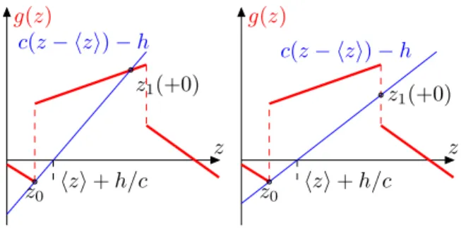
) i does not exist apart from the case h = 0. Hence, in this case the interface is never pinned, in agreement with our result from perturbation theory. The situation is different in the case when the random force exhibits infinite slopes as is shown in Fig. 1.3. Then, due to the discontinuities there are in general several solutions z _i for any value of c from which the leftmost ones dominate the behavior in the neighborhood of the depinning threshold. Of course, the larger the value of c the smaller is the fraction of disorder realisations which allow for more than one force free solution. Thus, for large c, the depinning threshold is diminished but finite. The presence of infinite slopes is a special feature of disorder forces, the correlator of which has a cusp singularity at the origin. A detailed analysis of the cusped disorder, as is sketched in Fig. 1.3 is presented in App. A.2, where we discuss how such a class of disorder forces can be realised and derive the correlator explicitly.

To test these predictions, we have solved equation (1.15) numerically. The depinning threshold h p is plotted in Fig. 1.4 as a function of c. It is clearly seen that the threshold increases with c

¹ , it vanishes for c > c _c for smooth random force correlations. For cusp correlations c _c → ∞ . These findings support the results from perturbation theory.

Scaling behaviour above depinning - general considerations

Now, we consider the behaviour slightly above the depinning threshold h & h _p , when h z i = vt but v ≪ 1. Our goal is to work out the scaling exponent β for the sliding velocity v, which we anticipate to vanish as a power law

v ∼ (h − h p ) ^β . (1.23)

To this aim, we solve the equation of motion in an approximate manner. As the velocity of the interface is small, v ≪ 1, we can also expect that ∂ _t z ≪ 1 for most of the time. Thus, z(t) follows essentially from the vanishing of the righthand side of (1.16), which means that z(t) stays close to the leftmost fixed point z ₁ (t). Since the disorder averaged position h z i is in motion, we have to keep in mind, that the root of the straight line in Figs. 1.2 and 1.3 is now moving relative to g(z). The intersection point z ₁ (t) satisfies the relation

z ₁ (t) = vt + c

¹ (h + g(z ₁ (t))). (1.24)

Without loss of generality, we restrict ourselves to v > 0, so z ₁ (t) moves now to the right. In

this part of the motion, z ₁ changes slowly (of order v). Eventually, z ₁ merges with z ₂ . Let us

assume that this happens at t = 0. For further reference we denote

z ₀ ≡ z ₁ ( − 0) = z ₂ ( − 0). (1.25)

For t > 0, these two solutions disappear and the intersection point z ₃ ( − 0) becomes the new leftmost intersection point, i.e. z 3 ( − 0) → z 1 (+0), so effectively z 1 jumps instantaneously.

Thus, at t > 0, the position z(t) is not any more close to a force free position and therefore it moves faster to approach the new intersection point z ₁ (t). The idea is now, that the mean velocity v is mainly determined by those disorder realisations, which move fast. In order to determine the scaling exponent β of v, it is thus our task to work out a quantitative description of the motion of a particle in a certain disorder realisation during a period of time between two collapses of force-free points. The temporal distance between two jumps of the leftmost force-free position is approximately given by

T = v

¹ , (1.26)

because this is the time needed to travel through a correlated region of the disorder (the length of which is of order O (1)). We denote the distance to the new leftmost intersection point z ₁ (t) by

θ(t) = z(t) − z ₁ (t). (1.27)

Note, that by definition θ(t) is negative. Now, Eq. (1.24) yields the identity

0 = h z(t) − vt i = 1 T

T

Z

0

dt h z ₁ (t) + θ(t) − vt i = 1 T

T

Z

0

dt h c

¹ h + c

¹ g(z ₁ ) + θ(t) i . (1.28)

Using Eq. (1.22), we obtain from (1.28) h − h p

c = − 1 T

Z T

0

dt h θ(t) i . (1.29)

The integral on the righthand side of (1.29) depends on the velocity. But, in order to use Eq.

(1.29) to determine the scaling exponent, we have to describe the interface motion for t > 0, i.e. in the region of the fast motion between the previous and the new force free position. We are going to do this separately for the two types of disorder considered in this section.

Scaling theory for disorder with a smooth correlator

The motion of the interface position after the collaps of the two leftmost force-free points is best analysed in several steps. First of all, we note that at t = 0 when z 1 and z 2 merge, the relation

c = g

(z ₀ ) (1.30)

holds. For t & 0, we can expect that z(t) is still close to z ₀ , so we can expand (1.16) around z 0 . Writing

ζ(t) = z(t) − z 0 (1.31)

and using (1.30), we obtain

∂ t ζ = cvt + g

(z 0 )

2 ζ ² + O (ζ ³ ), ζ(0) = 0. (1.32) For small ζ , we can neglect the second term on the righthand side and obtain

ζ(t) ≈ cvt ² /2. (1.33)

On time scales t ≥ t ₀ = 2[cvg

(z ₀ )]

the second term on the righthand side of (1.32) domi- nates the time evolution and we obtain

ζ(t) ≈ 2

g

(z ₀ )(t _d − t) , t _d = 3

2 t ₀ . (1.34)

Clearly, this result can only be used until a time t ₁ ≃ t _d − 2

g

(z ₀ ) , (1.35)

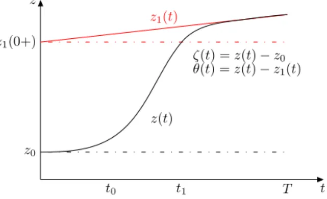
for which ζ(t ₁ ) . 1 since we made an expansion in ζ. It shows, however, that for t ₀ . t . t ₁ the coordinate z increases rapidly until it comes close to the new leftmost minimum z ₁ (t). For t > t 1 , θ(t) is already close to zero and therefore gives only higher order contributions to the righthand side of Eq. (1.29). The motion in between two jumps is sketched in Fig. 1.5

t z

z

z

(0+)

t

t

T

z

(t)

z(t)

ζ(t) = z(t) − z

θ(t) = z(t) − z

(t)

Fig. 1.5: Illustration of the motion z(t) in between two jumps in the case of smooth disorder.

Now, we are going to evaluate the integral over θ(t) that occurs in Eq. (1.29). The equations (1.27) and (1.31) relate θ(t) and ζ (t)

θ(t) = ζ(t) + z ₀ − z ₁ (t). (1.36)

The time dependence of z ₁ (t) can be estimated from Eq. (1.24) as

∂ _t z ₁ (t) = v + c

¹ g

(z ₁ (t))∂ _t z ₁ (t) ⇒ ∂ _t z ₁ (t) = cv

c − g

(z ₁ (t)) = cv

γ + O (v ² ), (1.37) where we have introduced γ = [c − g

(z ₁ (0+))] for notational convenience. Since z ₁ (0+) is a stable fixed point, we have γ > 0. Using

z ₀ − z ₁ (t) ≃ θ(0) − cv

γ t, (1.38)

we obtain

t

Z

0

dt θ(t) =

t

Z

0

dt

ζ (t) + θ(0) − cv γ t

= cvt ³ ₀

6 + t ₀ θ(0) − cv γ

t ² ₀ 2

= 2v

θ(0)[cg

(z 0 )]

+ O (1). (1.39) Further, for t ₀ < t < t ₁ , we have

t

Z

t

dt θ(t) =

t

Z

t

dt

ζ(t) + θ(0) − cv γ t

= 2

g

(z ₀ ) ln t _d − t ₁

t _d − t ₀ + θ(0)(t ₁ − t ₀ ) − cv γ

t ² ₁ − t ² ₀ 2

= v

θ(0)[cg

(z ₀ )]

+ O (ln v). (1.40) As we have already said, the integral over the remaining time t ₁ . . . T contributes to O (1) only.

Thus, up to orders O (v ln v), from (1.39) and (1.40) the expression on the righthand side of Eq. (1.29) follows as

1 T

Z T

0

dt h θ(t) i ≃ − v

3 D

| θ(0) | [cg

(z ₀ )]

E

. (1.41)

From (1.29) and (1.41), we obtain therefore

v ∼ (h − h _p ) ^3/2

c , (1.42)

i.e. β = 3/2.

Scaling theory for disorder with a cusped correlator

As we have mentioned before, if ∆(z) has a cusp singularity, the typical disorder force realisa-

tion exhibits discontinuous jumps, as is depicted in Fig. 1.3. A moment reflection shows, that

a merging of two force free solutions z ₁ and z ₂ is only possible at such a discontinuity of the

force field. The requirement, that z ₁ is a stable fixed point entails that such a discontinuity is

given by an upward jump in the force field. For the calculation we have to distinguish several

cases.

c(z − hzi) − h

hzi + h/c

c(z − hzi) − h

hzi + h/c

z

z

z

(+0) z

(+0)

z g(z)

z g(z)

Fig. 1.6: Left: This picture corresponds to our assumption for case 1 that the new intersection point z

(+0) is left of the next discontinuity of the disorder force g(z). It is obvious, that the inequality (1.43) has to be fulfilled. Right: A scenario contrary to case 1 is possible. However, the basic fact that the particle moves from the very beginning with a velocity g(z) − [c(z − h z i ) − h] = O (1) and therefore needs a time t

= O (1) to approach z

(+0), remains unchanged. So does the exponent β .

Case 1: In this case we assume, that the next stable intersection point occurs before the next discontinuity. Then, we have the inequality (cf. Fig. 1.6)

c > g

(z 0 +). (1.43)

It turns out that we have to solve the equation of motion in two time regimes. First, close to t = 0, z(t) is in the vicinity of z 0 and we consider again the equation for

ζ(t) = z(t) − z ₀ . (1.44)

Now, since the merging of two fixed points occurs at the discontinuities of the potential, Eq.

(1.30) is not meaningful, but instead z ₀ fulfills the equation

cz ₀ = g(z ₀ − ) + h. (1.45)

Using Eq. (1.45), it is easy to see that the equation of motion for ζ(t) takes the form

∂ _t ζ(t) ≈ c(vt − z ₀ ) + g(z ₀ +) + (g

(z ₀ +) − c)ζ + h = cvt − (c − g

(z ₀ +))ζ (t) + δg. (1.46) Here, δg = g(z ₀ +) − g(z ₀ − ) denotes the jump of g(z) which is of order one. Integration of (1.46) gives for short times t & 0

ζ(t) ≈ δg t. (1.47)

This result is approximately correct for t < t ₀ with

t ₀ = (c − g

(z ₀ +))

¹ . (1.48)

Note, that due to (1.43) the time t ₀ is always finite and positive, in fact generically of order O (1). For t > t ₀ , also the term in Eq. (1.46) proportional to ζ (t) becomes relevant. Now, z ₀ + ζ (t ₀ ) has to be compared with z ₁ (+0) which is the new leftmost intersection point for t > 0. From (1.24) we deduce that z ₁ (+0) fulfills the equation

cz ₁ (+0) ≈ h + g(z ₀ +) + g

(z ₀ +)(z ₁ (+0) − z ₀ ), (1.49)

from which we obtain

z ₁ (+0) ≈ h + g(z ₀ +) − g

(z ₀ +)z ₀

c − g

(z ₀ +) = [c − g

(z ₀ +)]z ₀ + δg

c − g

(z ₀ +) = ζ(t ₀ ) + z ₀ = z(t ₀ ). (1.50) In the second step, we have replaced h using Eq. (1.45). Thus, after the time t ₀ the particle has reached already the new intersection point z ₁ .

To determine the exponent β, we want to employ equation (1.29) again. For t ≤ t 0 , the relevant function θ(t) as has been obtained so far reads

θ(t) = z 0 − z 1 (t) + ζ(t) ≈ z 0 − z 1 (t) + δgt. (1.51) To approximate the time dependence of z 1 (t), we expand z 1 (t) around z 1 (+0) and get

z ₁ (t) ≃ z ₁ (+0) + ˙ z ₁ (0)t. (1.52) Here, ˙ z ₁ (0) can be deduced from the defining equation (1.24), it follows as ˙ z ₁ (0) = cvt ₁ with

t ₁ = (c − g

(z ₁ (0)))

¹ . (1.53) Thus, in the regime where θ(t) changes fast, i.e. for t ≤ t ₀ , we can write

θ(t) ≈ z ₀ − z ₁ (t) + ζ (t) ≃ δg(t − t ₀ ) − cvt ₁ t. (1.54) This shows, that for t > t 0 , θ(t) = O (v). However, the time scale t 0 is of the order O (1), and is thus small compared to T , t ₀ ≪ T . Therefore, it is important to carefully analyse the function θ(t) also for t > t ₀ . For t > t ₀ we expand around z ₁ (t) and the approximated equation of motion reads

∂ _t z ≃ c(vt − z) + g(z ₁ ) + g

(z ₁ )(z − z ₁ ) + h = − 1 t 1

θ(t), (1.55)

where t ₁ is defined in (1.53). Then, using (1.24) and (1.27), we find

∂ _t θ ≃ − 1

t ₁ θ(t) − cvt ₁ . (1.56)

The solution to this equation, matching with equation (1.54) gives

θ(t) ≈ − cvt ² ₁ + cvt ₁ (t ₁ − t ₀ ) e

^(t

^t

^)/t

. (1.57) The motion z(t) in between two jumps is sketched in Fig. 1.7

Now, we can determine β using equation (1.29). In calculating

− 1 T

Z T

0

dt h θ(t) i ≃ v δgt ² ₀

2 + ct ² ₁

+ O (v ² ), (1.58)

t z

z

z

(0+)

t

t

t

T

z

(t)

z(t)

z

(t) ζ(t) = z(t) − z

θ(t) = z(t) − z

(t)

Fig. 1.7: Illustration of the motion z(t) in be- tween two jumps in the case of disorder with a cusped correlator. The difference between the ab- sence (case 1, solid line) and the presence (case 2, dashed line) of a discontinuity of the force field g(z) in between z

and z

(0+) is the appearance of a sharp kink in the curve z

(t) at t = t

.

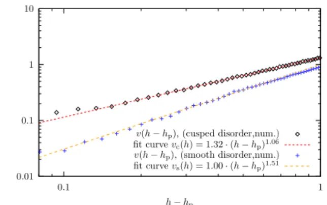
0.01 0.1 1 10

0.1 1

v

h−h_p

v(h−h_p), (cusped disorder,num.) fit curvev_c(h) = 1.32·(h−h_p)^1.06 v(h−h_p), (smooth disorder,num.) fit curvev_s(h) = 1.00·(h−h_p)^1.51

Fig. 1.8: The velocity as a function of h − h

for c = 0.67 in a double logarithmic plot. The numer- ically determined exponent for this measurement is β = 1.06 ± 0.08 for cusp-like singularity of ∆ (diamonds) and β = 1.51 ± 0.08 for smooth force correlation (crosses).

we have decomposed the integral into the intervals 0 . . . t ₀ and t ₀ . . . T , respectively. This gives v ∼ h − h _p

c , (1.59)

from which we conclude, that in the case of cusped disorder the velocity exponent is β = 1.

Case 2: Now, we have to discuss what can change if there is a discontinuity of g(z) in between z ₀ and z ₁ (0+). One possible scenario for this case is depicted in the right part of Fig.

1.6. We are going to discuss now, that our main result β = 1 remains unchanged. Indeed, as can be concluded from our previous calculation, the essential point that lead to the exponent β = 1 was the fact, that z(t) approaches z ₁ (+0) on a time scale t ₀ which is of order O (1).

Responsible for this is, that immediately after a collapse of the leftmost intersection point, the particle starts to move with a velocity of order δg = O (1). This remains unchanged. In Fig.

1.7 we have also sketched the motion when a discontinuity occurs in between z ₀ and z ₁ (0+).

The respective quantities in Fig. 1.7 carry a prime. The only effect of the discontinuity that is crossed at a time t

_j is a singularity of the velocity ˙ z

(t) at t = t

_j . The fundamental characteristics of the motion remain unchanged.

Thus, in case of k jumps of g(z) the foregoing calculation remains basically unchanged, apart from the fact, that one should now decompose the motion in one more parts: 0 . . . t j

; t _j

. . . t _j

; . . .; t _j

. . . t ₀ ; t ₀ . . . T . The first k pieces of the motion yield contributions to the integral (1.29) which are clearly all of the same type. Of course, this consideration changes the prefactor in Eq. (1.59), which is, however, anyway beyond our accuracy.

The two exponents β = 3/2 for smooth and β = 1 for cusped disorder are confirmed by

our numerical solution as depicted in Fig. 1.8.

1.3.2 Finite Frequencies

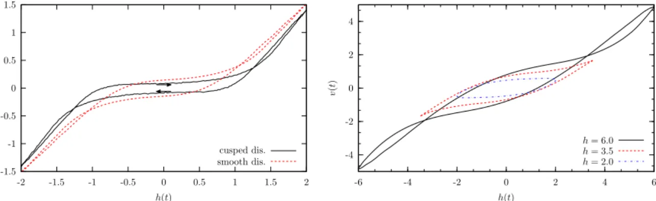
In the finite frequency case, the disorder average over the solutions to the equation of motion (1.11) forms a hysteresis in the v-h-plane, as is illustrated in Fig. 1.9 for the two types of disorder considered here.

-1.5 -1 -0.5 0 0.5 1 1.5

-2 -1.5 -1 -0.5 0 0.5 1 1.5 2

v(t)

h(t)

cusped dis.

smooth dis.

Fig. 1.9: In the presence of an ac driving field, a velocity hysteresis emerges. In this picture we illustrate these hystereses for the cusped and the smooth disorder for c = 0.5, h = 2.0 and ω = 0.1.

The inner hysteresis is traversed clockwise, the outer loops are passed through counter-clockwise

-4 -2 0 2 4

-6 -4 -2 0 2 4 6

v(t)

h(t)

h= 6.0 h= 3.5 h= 2.0

Fig. 1.10: The double hysteresis is only present for large enough driving field amplitudes. For small h, there is only a single hysteresis loop. This plot has been achieved for smooth disorder with the parameters c = 1.0 and η = 2.5, where t and z are measured in units such that ω = ℓ = 1.

The hystereses are invariant under the transformation v → − v and h → − h. This can be explained directly using the equation of motion (1.11) and a statistical inversion symmetry.

Taking the disorder average of (1.11) yields

∂ _t h z i = v = h cos ωt + h g(z(t)) i . (1.60) It is easy to see, that the aforementioned symmetry under v → − v and h → − h holds true if the probability density P [g] (cf. Eq. (1.10)) obeys P [g] = P [ˆ g] where ˆ g(z) = − g( − z). This is obviously the case for our assumption of Gaußian disorder.

An interesting consequence of this symmetry is, that the even Fourier coefficients of the solution v(t) (which is periodic with period 2π/ω) vanish. Once the steady state is reached, the symmetry requires v(t) = − v(t + π/ω). For the even Fourier modes this means

c _2N =

2π

Z

0

dt v(t)e ^{i2N ωt} =

π

Z

0

dt v(t)e ^{i2N ωt} +

π

Z

0

dt v t + π

ω

e ^{i2N ωt} = 0. (1.61)

As the frequency is sent to zero ω → 0, the hysteretic trajectory approaches the depinning

curve for an adiabatic change of the driving field that we have discussed in the previous

subsection. This is shown in fig. 1.11. Moreover, the effect of large c is to reduce the effect of

disorder. Clearly, for c → ∞ we have h z(t) i = z(t) and hence after averaging over the disorder

one finds h z i (t) = (h/ω) sin ωt and v(t) = h(t) as expected. Thus, for large c the hysteresis

winds tightly around the diagonal.

-6 -4 -2 0 2 4 6

-6 -4 -2 0 2 4 6

v(t)

h(t)

ω= 1.0ω₀ ω= 0.1ω0

Fig. 1.11: Numerical solution of equation (1.11) for h = 6.0, c = 1.0 and η = 2.5 for different frequencies and smooth disorder, t and z being measured in units such that ω

= ℓ = 1.

-40 -20 0 20 40

-40 -20 0 20 40

v(t)

h(t)

c= 1.0 c= 10.0

Fig. 1.12: Numerical solution of equation (1.11) for different elastic constants and h = 40.0, η = 10.0. The disorder is smooth and the units of t and z are chosen such that ω = ℓ = 1.

Qualitative discussion of the motion

To understand the shape of the hysteresis, we consider the motion of a particle for half of a period for the case h ≫ h _p and small frequency ω ≪ c. We start at a time t = 0, when h(0) = − h _p and the field increases. Then, we can expect each particle to be located close to the rightmost force free point, i.e. the rightmost solution of

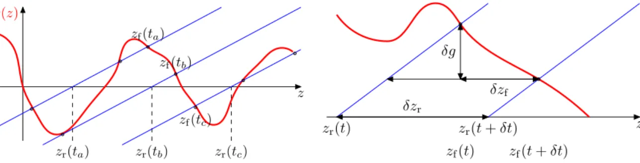
c (z _f (t) − h z i (t)) − h(t) = g(z _f (t)). (1.62) In Fig. 1.13 it is illustrated, that due to the change of the driving field towards larger values,

z

(t

) z

(t

)

z

(t

) z

(t

) z

(t

) z

(t

)

z g(z)

Fig. 1.13: At h(t

) ≈ − h

, the particle is close to the rightmost force free point z

(t

). This inter- section point moves, due to the change of the zero z

(t) = h z i (t) + h(t)/c. The particle is following this point. At a later time t

, when h(t

) ≈ h

this force free point has become the leftmost one.

δz

δz

δg

z

(t) z

(t + δt)

z

(t) z

(t + δt) z

Fig. 1.14: Illustration for the velocity estimate.

The motion of the root z

of the straight line c(z − h z i ) − h entails a change in z

, that can be easily estimated in terms of simple trigonometry.

the root of the straight line, given by

z _r ≡ h z i (t) + h(t)/c (1.63)

moves with a velocity

˙

z r = v(t) + h(t) ˙

c . (1.64)

Since ˙ h(t) > 0, this velocity is positive although the value of the field is still negative. There- fore, also the intersection point z _f (t) to which the particle is connected, moves to the right.

This fact is observed in the hysteresis loop, illustrated in Fig. 1.9. Actually, this understand- ing allows to estimate the velocity in simple geometrical terms. Using the notation explained in Fig. 1.14, we have δg/δz _f ≃ g

(z _f ) and thus

δz r − δz _f = − δg

c = − g

(z _f )δz _f

c , ⇒ δz r = c − g

(z _f )

c δz _f . (1.65)

Now, Eq. (1.64) yields

δz _r

δt = c − g

(z _f ) c

δz _f δt ≃ δz _f

δt + h(t) ˙

c . (1.66)

Solving the last approximate equality for δz _f /δt, we obtain

˙

z _f ≃ − h/g ˙

(z _f ). (1.67)

During the motion of z _f (t), other intersection points to the left of z _f (t) vanish, and new solutions to the right emerge. Finally, when h(t ₁ ) ≈ h _p , z _f (t ₁ ) has become the leftmost intersection point. From approximately this time on it happens, that occasionally in some disorder realisations z _f (t) merges with an unstable fixed point and vanishes, so that the particle moves fast in order to catch up with the new leftmost force free point. This procedure has already been discussed earlier in Sec. 1.3.1. Since the velocity of a particle is given by the difference between g(z) and the straight line c(z − h z i ) − h, it must fall back behind the leftmost intersection point to speed up. This can only happen due to the disappearance of force free points. Thus, the velocity grows slowly because after each jump the particle moves fast and thus approaches again the new intersection point. On the other hand, by virtue of Eq. (1.64), the larger v(t) the faster z _r (t) and thus also the faster the intersection points move.

This leads to a positive feedback and entails a strong slope when the velocity is large enough

such that the particle is no longer able to approach a force free point before the next jump

sets in. Finally, far above h _p the particle is depinned. After the driving force has reached its

maximum it decreases. Note that the root of the straight line z _r has now a velocity smaller

than v(t), because ˙ h is negative. Therefore, the particle position z(t) approaches z r (t) and

slows down. Hence, ˙ h is a measure also for the decrease of v(t). On approaching h _p from

above, all particles are still depinned and hence far enough behind the leftmost intersection

point, so that the latter has only little influence on the motion of the particle and the velocity

decays with the same slope all the time. Only when v(t) has passed below ˙ h/c, z _r moves in

the negative direction and thus the intersection points as well. This means, that the leftmost

intersection point approaches the particle before it is pinned. After the particle is a little to

the right of the leftmost force free position, which happens about when h(t) ≈ h _p , the velocity

is negative. Now, the same procedure starts in the other direction.

As ω → 0, the hystereses approach the depinning curve that has been discussed in the previous chapter. In the following, we are going to take a closer look on the details of this limiting process.

Velocity exponents

First, we want to work out, how

v _h

≡ | v(h = 0) | (1.68)

approaches zero as ω → 0. As we have explained in Sec. 1.3.2, the particle in each disorder realisation stays close to a force-free point, that we have agreed to label z _f (t). The velocity

∂ _t z of the particle is now determined solely by the velocity of the force free position z _f that we are now going to calculate in a more accurate way than our estimate from Eq. (1.67). Let t 0 be the point in time, at which h(t 0 ) = 0. On time scales that are small compared to the period ω

¹ , we can linearly expand the driving field around t ₀

h(t) ≃ − hω(t − t 0 ). (1.69)

Further, we want to expand (1.62) around z _f (t ₀ ). For small distances in time we can neglect possible changes in the velocity and write

z _f (t) ≃ z _f (t ₀ ) + v _f (t − t ₀ ), (1.70) where v _f = ∂ _t z _f is a shorthand notation. Using (1.69) as well as h z i (t) ≃ h z i (t ₀ ) − v _h

(t − t ₀ ), we have

0 =c

z _f (t ₀ ) + v _f (t − t ₀ ) − h z i (t ₀ ) + v _h

(t − t ₀ )

+ hω(t − t ₀ ) − g(z _f (t ₀ )) − g

(z _f (t ₀ ))v _f (t − t ₀ )

=(t − t 0 )

c(v _f + v _h

) + hω − v _f g

(z _f (t 0 ))

(1.71) Since this should hold for small but finite | t − t ₀ | , the expression in the rectangular brackets has to vanish. Solving (1.71) for v _f , taking the disorder average and using the self-consistency condition h v _f i = − v _h

finally yields

v _h

= − hω

c − h [c − g

(z _f (t ₀ ))]

¹ i

¹ . (1.72) Since g

(z _f (t ₀ )) < 0, which expresses the reasonable assumption that z _f is a stable force free position, v _h

is indeed positive, which must be the case by its definition (1.68). Note, that our derivation so far does not make any assumption about the disorder correlator, whence it holds for cusped as well as for smooth disorder. In conclusion, for ω → 0 the width of the hysteresis at h = 0 behaves as v _h

∼ ω ^κ with κ = 1 for either kind of disorder. This exponent is verified by our numerical analysis, cf. figure 1.15.

Another interesting quantity to look at is

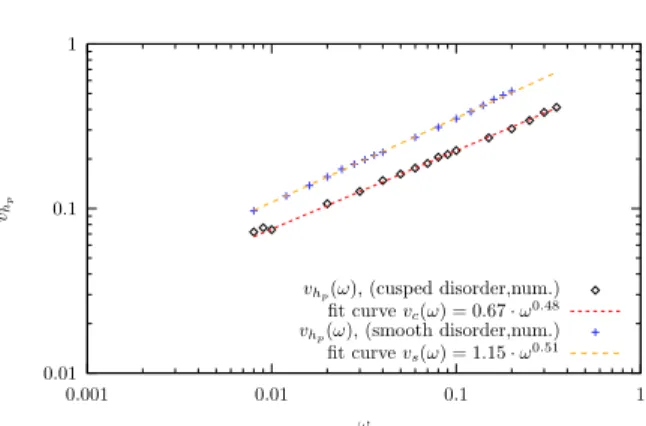
v _h

≡ | v(h = h _p ) | , (1.73)

0.001 0.01 0.1 1

0.001 0.01 0.1 1

vh0

ω

v_h0(ω), (cusped disorder,num.) fit curvev_c(ω) = 0.9·ω^0.97 v_h0(ω), (smooth disorder,num.) fit curvev_s(ω) = 1.5·ω^0.95

Fig. 1.15: The velocity v

as a function of fre- quency. The plotted data correspond to numerical measurements at c = 0.33 for cusped and c = 0.2 for smooth disorder. For either type of disorder, the exponent is close to 1 (κ

= 0.97 ± 0.07 and κ

= 0.95 ± 0.04) in agreement with our analytical derivation given in the main text.

0.01 0.1 1

0.001 0.01 0.1 1

vhp

ω v_h

p(ω), (cusped disorder,num.) fit curvev_c(ω) = 0.67·ω^0.48 v_h

p(ω), (smooth disorder,num.) fit curvev_s(ω) = 1.15·ω^0.51

Fig. 1.16: The velocity v

as a function of fre- quency. The plotted data correspond to numerical measurements at c = 0.33 for cusped and c = 0.2 for smooth disorder. For both types of disorder, the exponents are close to 1/2 (µ

= 0.48 ± 0.02 and µ

= 0.51 ± 0.01).

of which we want to work out the limiting behaviour for ω → 0. As h(t) increases further from 0 towards h _p , more and more of the force free points z _f , which the true positions in the disorder realisations are following, become the rightmost ones, so that occasionally jumps occur. On closely approaching h(t) = h _p the dominant contribution originates from these jumps, which severely affects the exponent, so that v _h

∼ ω ^µ with µ ≃ 1/2, as can be inferred from our numerical analysis, shown in figure 1.16. This exponent is again independent of the shape of the disorder correlator at the origin (smooth or cusped). An analytical derivation of this exponent is much more complicated than it was the case for κ and in fact we did not find a rigorous prediction. For the finite dimensional case in 4 − ǫ dimensions, the exponent µ has been found as µ = β/(νz), where ν denotes the correlation length exponent and z the dynamical exponent [38].

The area of the hysteresis loop

Next, we want to investigate the limiting behaviour of the hysteresis area. The physical meaning of the loop area can be concluded from the energy balance of an overdamped system.

For the change of the disorder averaged potential energy in time, we find (cf. App. A.3)

∂ t h E i = h(t)v(t) − (∂ t z) ²

. (1.74)

Here, h(t)v(t) measures the energy gain through the work per unit time that is done by the external field and

(∂ _t z) ²

measures the energy loss per unit time due to dissipation. The area of the hysteresis loop is determined via

A _hyst (ω) = I

v(t) dh = Z T

0

v(t) ˙ h(t) dt. (1.75)