The Roles of Demographic Changes on Labor Market Dynamics and Consumption
Inequality
Inauguraldissertation zur Erlangung des Doktorgrades der Wirtschafts- und Sozialwissenschaftlichen Fakultät der
Universität zu Köln
2019
presented by
M.A. Yu Han
from
Henan, China
First reviewer: Prof. Michael Krause, Ph.D.
Second reviewer: Prof. Dr. Johannes Pfeifer Date of oral defense: March 11, 2019
To my parents, my lovely wife,
and my son
Acknowledgements
I am sincerely grateful to my advisor, Michael Krause, for his supervision and guidance from the very early stage of this research. He always had time for me, and has spent many hours discussing my ideas. One could not wish for a better or friendlier advisor. I would also like to show my deepest gratitude to my second advisor, Johannes Pfeifer, for his excellent advice at the very critical stage of this research. His willingness to read multiple versions of this thesis has far exceeded my expectation. I have benefited enormously from his sharp, insightful, and invaluable comments. Without their most generous encouragement and support, this thesis would not have been possible.
I deeply appreciate the comments from my colleagues at the Center for Macroeconomic Research and our academic visitors. Above all, I wish to thank Christopher Busch, Alexander Ludwig, and Davide Debortoli for the time they spent on discussing the paper covered in Chapter 3, Jonas Löbbing and Noam Yuchtman for their valuable feedback on the paper covered in Chapter 4.
I also benefited a lot from our faculty members and other colleagues at the CMR. In particular, I am grateful to Christian Bredemeier, Emanuel Hansen, Peter Funk, Erik Hornung, Thomas Schelkle, Helge Braun, Christoph Kauf- mann, and Matthias Schön for their generous help in improving my presentation skills. Furthermore, I give my special thanks to my good friends Fangjian Gao, Matthias Götz, Dila Asfuroglu, and Raphael Flore for the wonderful memories at the Cologne Graduate School.
My study here was made possible by financial support from the University of Cologne. I explicitly thank Dagmar Weiler for her support via the CGS and Andreas Schabert for his support via the CMR. I also like to thank Erika Berthold, Ina Dinstühler, Diana Frangenberg, Sylvia Hoffmeyer, and Dorothea Pakebusch for their generous support.
v
Most importantly, I want to thank my wife Sangsang and my parents for their love and support throughout this research. Sweet thank is to my son Heyi for enlightening my life.
Contents
1 Introduction 1
2 Demographic Changes and Unemployment Volatility 5
2.1 Introduction . . . 5
2.1.1 Related literature . . . 8
2.2 Measure of unemployment volatility . . . 10
2.2.1 Data . . . 12
2.3 Unemployment volatility by age . . . 13
2.4 Empirical identification of the role of demographic changes . . . 17
2.4.1 Unemployment volatility of young workers . . . 17
2.4.1.1 Time series properties . . . 18
2.4.1.2 Regression results . . . 21
2.4.2 Unemployment volatilities of prime-age and old workers . 25 2.4.3 Aggregate unemployment volatility . . . 26
2.4.3.1 Changes in composition of the sample and redef- inition of the age group . . . 27
2.5 Decomposition of the effect of demographic changes in the Great Moderation . . . 29
2.6 Conclusion . . . 32
3 Demographic Structure and the (Un)employment Volatility of Young Workers 35 3.1 Introduction . . . 35
3.2 Empirical evidence . . . 39
3.2.1 The role of labor force participation . . . 40
3.2.2 Identifying the role of demographic changes . . . 42 vii
3.3 The model . . . 44
3.3.1 Households . . . 44
3.3.2 Labor markets . . . 45
3.3.3 Firms . . . 47
3.3.4 Characterization of agents’ asset values . . . 48
3.3.5 Comparative statics and the youth share . . . 50
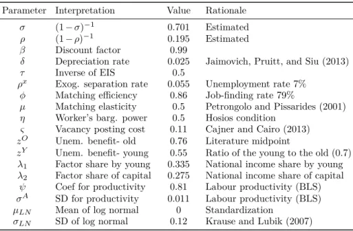
3.4 Calibration . . . 54
3.4.1 The two parameters governing the elasticities of substitution 54 3.4.2 Other parameters . . . 55
3.5 Simulation results . . . 57
3.5.1 Aggregate volatility across demographic states . . . 58
3.5.2 Age-specific volatility across demographic states . . . 59
3.5.3 Dynamic response of labor market variables of the young 61 3.6 Introducing exogenous separation . . . 63
3.7 Empirical assessment of the mechanism . . . 66
3.8 Summary . . . 68
4 Population Aging, Monetary Policy, and Consumption Inequal- ity 69 4.1 Introduction . . . 69
4.2 The model . . . 74
4.2.1 Households . . . 74
4.2.1.1 Retirees . . . 74
4.2.1.2 Workers . . . 76
4.2.1.3 Aggregation . . . 78
4.2.2 Firms . . . 80
4.2.2.1 Final goods producers . . . 80
4.2.2.2 Intermediate goods producers . . . 81
4.2.3 Capital producers . . . 82
4.2.4 Government’s policy . . . 84
4.2.4.1 Fiscal policy . . . 84
4.2.4.2 Monetary policy . . . 84
4.2.5 Market clearing . . . 84
4.2.6 Equilibrium . . . 85
4.3 Calibration . . . 85
CONTENTS ix
4.4 Simulation results . . . 87
4.4.1 Transition path . . . 88
4.4.2 The asymmetric dynamic effects . . . 91
4.4.2.1 Preference shock . . . 91
4.4.2.2 Monetary shock . . . 93
4.4.2.3 The effects of the ZLB under an older demo- graphic structure . . . 94
4.4.3 Extension of retirement age . . . 95
4.5 Conclusion . . . 97
A Appendices to Chapter 2 99 A.1 Specification of Equation (2.1) . . . 99
A.2 Data sources . . . 100
A.3 Summary statistics of key variables . . . 101
A.4 Time-varying unemployment volatility by age group for other six- teen countries . . . 102
A.5 Calculation of test statistics . . . 104
A.6 The role of labor market institutions in the unemployment volatil- ity of young workers . . . 105
A.7 CCEMG estimators for prime-age and old workers . . . 106
A.8 Redefinition of age group: the young (15-29) . . . 106
B Appendices to Chapter 3 107 B.1 Participation’s share in unemployment volatility (with different age groups categorization) . . . 107
B.2 Unemployment volatilities of other age groups and demographic changes . . . 108
B.3 Proof of Proposition 1. . . 108
B.4 Proof of Proposition 2. . . 110
B.5 Derivation of the equations for ∂∂lnθlnAY and ∂∂lnulnAY in case of en- dogenous job separation . . . 112
B.6 (Linearized) equation system for model with endogenous separation115 B.7 Bellman equations for model with exogenous job separation . . . 119
B.8 Derivation of the equation for ∂∂lnθlnAY in case of exogenous job separation . . . 120
B.9 IRFs with respect to an aggregate productivity shock (with ex-
ogenous job separation) . . . 122
C Appendices to Chapter 4 123 C.1 Derivations of Euler equations for households and FOCs for final goods producers . . . 123
C.1.1 Retirees’ problem . . . 123
C.1.1.1 Derivation of the dynamic equations . . . 123
C.1.1.2 Verification of the conjecture of the value func- tion of retirees . . . 124
C.1.2 Workers’ problem . . . 125
C.1.2.1 Derivation of the dynamic equations . . . 125
C.1.2.2 Verification of the conjecture of the value func- tion of workers . . . 128
C.1.3 Final goods producer’s Problem . . . 128
C.2 Detrended system of equations . . . 129
C.3 Decomposition of dependency ratio . . . 132
C.4 Effects of population aging . . . 133
C.4.1 When retirees enjoy full leisure . . . 133
C.4.2 When retirees endogenously decide their labor supply . . 134
Bibliography 136
List of Figures
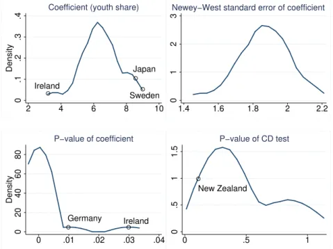
2.1 Time-varying unemployment volatility by age group . . . 15 2.2 Youth share and unemployment volatility of young workers . . . 18 2.3 Robustness: distribution of key parameters after dropping one
country at a time . . . 28 2.4 Decomposition of the effect of demographic changes in the Great
Moderation . . . 31 3.1 Unemployment volatility and the youth share (U.S.) . . . 36 3.2 Timing of events . . . 46 3.3 IRFs of variables of the young with respect to aggregate produc-
tivity shock across demographic states . . . 62 4.1 Demographic transition in the U.S. projected until 2060 . . . 70 4.2 Demographic processes in the model and in the data . . . 86 4.3 Simulations following different paths of demographic transition . 89 4.4 Impulse responses to a positive preference shock . . . 92 4.5 Impulse responses to an expansionary monetary policy shock . . 93 4.6 The IRFs of the relative consumption ratio to shocks under dif-
ferent demographic structures . . . 95 4.7 Transition paths of the relative consumption ratio and the real
interest rate after an extension of retirement age (65→67) . . . 96 A.1 Time-varying unemployment volatility by age group (1/2) . . . . 102 A.2 Time-varying unemployment volatility by age group (2/2) . . . . 103
xi
B.1 IRFs of variables of the young with respect to an aggregate pro- ductivity shock across demographic states (with exogenous sepa- ration) . . . 122 C.1 Decomposition of dependency ratio . . . 132 C.2 Response to a preference shock when retirees enjoy full leisure . . 133 C.3 Response to a monetary shock when retirees enjoy full leisure . . 134 C.4 Response to a technology shock with flexible labor supply from
retirees . . . 135 C.5 Response to a monetary shock with flexible labor supply from
retirees . . . 135
List of Tables
2.1 Cyclical volatility of unemployment by age group, 20 OECD coun- tries . . . 14 2.2 Specification tests . . . 20 2.3 Unemployment volatility and the share of labor force: young workers 21 2.4 Labor force participation and international migration: further ro-
bust check . . . 24 2.5 Unemployment volatility and the share of labor force: prime-age
and old workers . . . 26 2.6 Aggregate unemployment volatility and the share of labor force . 27 3.1 Decomposition of unemployment volatility: share of participation 41 3.2 Unemployment volatility of the young and demographic changes 43 3.3 Estimation results of the elasticities of substitution in final goods
production . . . 55 3.4 Parameter values in simulation (quarterly) . . . 56 3.5 Summary of the first moments in benchmark calibration (quarterly) 58 3.6 Aggregate second moments in the data and the model . . . 59 3.7 Age-specific second moments in the data and the model . . . 60 3.8 Further decomposition of unemployment volatility . . . 63 3.9 Second moments in the data and the model (with exogenous sep-
aration) . . . 65 3.10 The price of goods produced by the young and the share of the
young . . . 66 3.11 Second moments of the transition rates of the young over time . 67 4.1 Parameter Values in Simulation . . . 87
xiii
A.1 Unemployment volatility and demographic statistics . . . 101 A.2 Unemployment volatility and the share of labor force: young
workers - with the coefficients of LMIs . . . 105 A.3 Unemployment volatility and the share of labor force: prime-age
and old workers . . . 106 A.4 Unemployment volatility and the share of labor force: young
workers (15-29) . . . 106 B.1 Decomposition of unemployment volatility: participation’s share 107 B.2 Unemployment volatility and demographic changes: prime-age
and old workers . . . 108 C.1 Values under stationary population . . . 134
Chapter 1 Introduction
This thesis consists of three essays on the impacts of demographic changes on labor markets and consumption goods markets. More specifically, the first two essays examine the role of demographic changes on labor market dynamics with empirical evidence and a theoretical framework, respectively. The third essay investigates the differential impacts of demographic changes on the consumption of retirees and workers.
The impacts on labor market dynamics come from the substantial changes in the demographic composition of labor markets, which happen among the vast majority of developed economies. In the U.S., for instance, the share of young workers (aged 15–24 years) in the labor force, let us name it the youth share afterward, has increased from 19% since 1960s to 25% by the late 1970s due to the postwar baby boom. Recently, this value decreased to less than 15% as the inflow of young workers dwindled. In Japan, this value declined from 23% in the late 1960s to less than 10% currently. If workers at different age levels are disproportionately affected by the business cycle, then changes in the youth share will have a direct composition effect on aggregate labor market dynamics, even if age-specific labor market dynamics remain unchanged during demographic changes.
It is often thought that young workers would be more easily affected by the business cycle, as they lose jobs more often and their (un)employment rate is generally more cyclically sensitive. In the first essay, I first show that this guess is supported by data. In particular, the labor market volatility of young workers, in terms of unemployment volatility, is significantly higher than those of other age
1
groups, and the corresponding values of prime-age and old workers are relatively close. This age-specific difference points out the importance of demographic changes in accounting for aggregate business cycle volatility. Besides, I observe that there is a hump-shaped pattern in the youth share in the U.S. from 1960 to 2007, at the same time, aggregate unemployment volatility comoves with this youth share over time. More importantly, I find an even closer comovement between the unemployment volatility of young workers and this youth share.
This suggests a new channel: Unemployment volatility within the group of young workers increases with their share in the labor force.
I then test empirically this new channel. Using an unbalanced panel of 20 OECD countries from 1960 to 2007, I find that the variation in the youth share has a quantitatively large and statistically significant, positive effect on the unemployment volatility of young workers. The causality of this relationship is identified by the exogeneity of the youth share, as it is predetermined at least 15 years prior. I refer to this novel fact as a spillover effect.
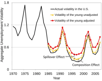
To quantify the relative importance of this spillover effect with respect to the composition effect as mentioned before, which is proposed as the only demo- graphic explanation for business cycle volatility by Jaimovich and Siu (2009), I decompose the overall effect of demographic changes on aggregate unemployment volatility. In contrast to Jaimovich and Siu (2009), I find that the spillover effect accounts for most of the effect of demographic changes. In accounting for “The Great Moderation”—the substantial decline in cyclical volatility experienced in the U.S. since the mid-1980s, I find that demographic changes can explain one quarter of the decline in unemployment volatility. Of this, the spillover effect ac- counts for two-thirds of the overall effect, while the composition effect accounts for only a third.
In the second essay, I explore a potential explanation of this novel fact. I argue that an increase in the youth share depresses the price of goods produced by young workers. This generates a congestion in their labor market dynam- ics and raise their cyclical unemployment volatility. To be specific, I build on Jaimovich, Pruitt, and Siu (2013) by incorporating a job matching model with endogenous job separation into the real business cycle model, to connect labor demand with the dynamics of labor market transition rates.
3 I start by distincting goods produced by young and old workers. Then, these two distinct goods are combined with capital for the production of final goods.
Therefore, this distinction generates a labor demand structure that differentiates between young and old workers. With this labor demand structure, a greater share of young workers is associated with a lower relative price of goods produced by them, lowering firms’ profits. This induces spillover effects in labor market dynamics, both in the job separation and finding rates. For the former, the volatility of the job separation rate increases with the youth share, because young workers become more vulnerable to productivity shocks. For the latter, the volatility of job finding rate also increases with the youth share, since firms’
vacancy posting also becomes more sensitive to productivity shocks, which works the same way as Hagedorn and Manovskii (2008). Therefore, both aspects imply that the unemployment volatility of young workers increases with the youth share.
As corroborating evidence for this mechanism, I find that the decline in the relative price of goods produced by young workers due to a greater share of young workers is supported by empirical data. Further evidence comes from the empirical dynamics of transition rates: The second moments of the transition rates of young workers are higher if the share of young workers is higher, and vice versa. This empirical pattern is exactly the same as my model predicts.
The dependence of the labor market dynamics of young workers on demo- graphic structure have important policy implications. First, it points out the necessity for policy-makers to pay attention to the current state of demographic structure and its projected path, if they need information about the labor market response to potential shocks, especially for young workers. Second, the positive correlation between business cycle volatility and demographic changes also sug- gests that the Great Moderation was more likely driven by structural factors other than good policies.
The third essay focuses on consumption goods markets, by assessing the dif- ferential impacts of demographic changes on the consumption of retirees and workers. The research topic is of particular interest, not only because of the increasing income and wealth inequality in industrialized countries in the past few decades (Piketty, 2015), but also because these countries will experience considerable growths in their older population while significant declines in their
working population. In the U.S., the dependency ratio—the number of popula- tion over 65 years to working age population, is expected to grow from 0.22 in 2015 to 0.40 in 2060. Some other countries have already stepped into the society of aging. In Japan, the dependency ratio is already up to 0.47 in 2017, almost three times as much as that in 1990. The current ratios for Italy, Germany, and France are all over 0.3.
Using a New Keynesian model featuring the life-cycle behavior of Gertler (1999), I predict an increase in consumption inequality between retirees and workers in the U.S., measured by the ratio of consumption per retiree to con- sumption per worker, using its projected demographic evolution. In my cali- brated model, this ratio is predicted to decline by 40% for the U.S., from 0.68 to 0.41, between 1990 and 2060, due to population aging. As the zero lower bound will bind more frequently with an older population, in addition, I also investi- gate the distributional effects of the zero lower bound during cyclical downturns.
I find that the presence of the zero lower bound can mitigate the asymmetric effects of shocks on workers and retirees in dynamics, because there is a lower decline in the real return on assets, which particularly benefits retirees.
Chapter 2
Demographic Changes and Unemployment Volatility
2.1 Introduction
The demographic composition of the labor market has changed substantially among developed economies. In the U.S., the persistent inflow of young workers (aged 15–24 years) into the labor market since 1960s has pushed the youth share, the share of young workers in the labor force, to be more than one quarter by the late 1970s, and then as the inflow dwindled, this value decreased to less than 15% recently. In Japan, the share of old workers (aged 55–64 years) in the labor force increased from 10% in the 1960s to more than 20% currently1. The implications of demographic changes in the labor market are far reaching.
In this paper, I focus on the effect of demographic changes on unemployment volatility.
It is often thought that young workers would be more easily affected by the business cycle, while the opposite is considered true for prime-age workers. My first contribution consists in showing that this guess is supported by data. There are sharp age-specific differences. In particular, the unemployment volatility of young workers is significantly higher than those of other age groups, and the corresponding values of prime-age and old workers are relatively close.
Given the size of the unemployment volatility of young workers, changes in the youth share have a direct composition effect on aggregate unemployment
1If the labor force is evenly distributed across age groups, the youth share will be 20%
and so will the share of old workers.
5
volatility. Ceteris paribus, more young workers in the labor force naturally mean higher aggregate unemployment volatility even if age-specific unemploy- ment volatility remains unchanged. The prediction of the impact of demographic changes would be a simple task if it was only due to the composition effect. But, if age-specific unemployment volatility is also affected by demographic changes, estimating the effect on each age group is of vital importance for precise pre- diction. Besides, the estimation results could have important implications for policy makers when it comes to coping with age-specific labor market policies.
My second contribution lies in showing that there is also a spillover effect among young workers. The variation in the youth share has a quantitatively large and statistically significantly positive effect on the unemployment volatility of young workers. This further contributes to the variation in aggregate unemploy- ment volatility. After decomposing the overall effect of demographic changes on aggregate unemployment volatility into composition and spillover effects, I find that the spillover effect accounts for most of the effect of demographic changes.
In accounting for “The Great Moderation”—the substantial decline in cyclical volatility experienced in the U.S. since the mid-1980s, I show that demographic changes can explain 24.2% of the decline in unemployment volatility. Of this, the spillover effect accounts for 16.6%, while the composition effect only 7.6%.
To measure unemployment volatility, I use time-varying volatility based on a stochastic volatility process with an autoregression (SV with AR) used in re- cent studies (see e.g. Fernández-Villaverde et al., 2011; Born and Pfeifer, 2014).
Compared with the rolling-window standard deviation, a conventional measure used in the literature (see e.g. Blanchard and Simon, 2001; Jaimovich and Siu, 2009; and Carvalho and Gabaix, 2013), it has two advantages: First, as a depen- dent variable, it does not suffer from serial correlation in the residuals, which is inevitable for the conventional measure that uses overlapping data for the con- struction of consecutive values. Second, it does not have any loss in the amount of observations, while for the other, a 10-year window period means a loss of nine observations for each country. Furthermore, in comparison with the instan- taneous standard deviation based on Stock and Watson (2003) (Stock/Watson) used in Jaimovich and Siu (2009), it is still preferred. For the measure based on Stock/Watson, the unit root assumption used for the variance equation is not
2.1. INTRODUCTION 7 empirically supported2. Besides, it uses a mixture of different normal distribu- tions for the shock in the variance equation to ensure a better fit with the data, but this practice makes it suffer from subjectivity in the selection of weights for this shock.
In addition to the demographic variable, which is used as the sole explana- tory variable in Jaimovich and Siu (2009), Lugauer and Redmond (2012), and Lugauer (2012b), I include labor market institutions to explain unemployment volatility. Union density and the centralization of wage bargaining reflect real wage rigidities, which play an important role in the amplification of unemploy- ment fluctuation (Hall, 2005). In addition, according to Hagedorn and Manovskii (2008), high unemployment benefit suggests a low value for firms’ profit, and therefore a high cyclical unemployment fluctuation. Neglecting the effects of la- bor market institutions might lead to biased estimation or even spurious regres- sion. Although changes in labor market institutions could also partially reflect demographic pressures, this does not affect the consistency of the estimation.
As pointed out by Everaert and Vierke (2016), the negligence of the time series property of panel data might lead to spurious inferences. In view of this, I also carry out extensive stationarity analyses on relevant series. Another reason is the relatively monotoneous variation in the demographics and unemployment volatility over the sample period. Hypothetically, the two could merely share a similar trend in coincidence. The results show that this possibility is excluded as stationarity tests reject the null hypothesis of a unit root in any of them.
But I detect cross-sectional dependence in both series. This could lead to biased upward stationarity statistics and falsely reject the null hypothesis. Thus, I also run panel cointegration tests to ensure the validity of regression results in case of non-stationarity. Besides, I use the common correlated effects (CCE) estimators proposed by Pesaran (2006) to take care of cross-sectional dependence.
2The estimates of the coefficient of the AR(1) process of the variance equation are smaller than unity for all countries in my sample. Therefore, the unit root assumption is not supported. Results are available upon request.
2.1.1 Related literature
This paper contributes to four strands of literature. First, this paper is closely related to the studies initiated by Jaimovich and Siu (2009) on the role of demo- graphic changes in aggregate business cycle volatility. By linking demographic changes to the aggregate cyclical volatility of real GDP after World War II in G7 countries, they claim that the change in the age composition of the labor force over time is the main demographic reason for the variation in aggregate cyclical volatility. As follow-ups, Lugauer and Redmond (2012) and Lugauer (2012b) also found similar results with, respectively, a balanced panel dataset for 51 countries and state-level data of the U.S. But the replication by Everaert and Vierke (2016) indicates that these regression results may be spurious, as the series used in these papers for demographic change and cyclical volatility are found to be non-stationary. Besides, no co-integrating relation is detected between these two series.
Building on these studies, this paper confirms the positive impact of demo- graphic changes on aggregate unemployment volatility. To obtain this result, I deviate from the literature in three aspects. First, I use the youth share as a measure for demographics instead of the compact index, which is the share of young and old workers in the labor force, used in Jaimovich and Siu (2009).
Although their analysis shows that the volatilities of hours worked and employ- ment for young and old workers are obviously higher than that of prime-age workers, it is too restrictive to assume the regression coefficients for the young and the old as being the same. This is because the underlying reasons are dif- ferent: The fact that the cyclical volatility of young workers is high is related to their low work experience, which is a persistent feature for young workers in most countries; for old workers, on the other hand, it depends on labor market reforms such as changes in the generosity of unemployment benefits and firing cost, which are heterogeneous in terms of timing and scale among different coun- tries. Second, I use the time-varying volatility based on SV with AR to measure unemployment volatility instead of a rolling-window standard deviation3 or the
3Besides, the rolling-window standard deviation in Jaimovich and Siu (2009) is filtered by Hodrick-Prescott (HP) filter. Since HP filter itself already has several flaws (see Hamil- ton, 2017), a volatility measure which further uses a rolling-window standard deviation is at a disadvantage.
2.1. INTRODUCTION 9 measure based on Stock/Watson used in Jaimovich and Siu (2009) with its ad- vantages mentioned before. In fact, with this measure, I find that the difference in unemployment volatility between old and prime-age workers is not a general worldwide phenomenon; this corroborates my first deviation. Finally, I also con- trol the effect of labor market institutions, which is overlooked in the literature and is likely to be the reason for the non-stationarity detected by Everaert and Vierke (2016) in the series used by Jaimovich and Siu (2009) and their follow-ups.
Despite there being rich literature on the impact of demographic changes on aggregate business cycle volatility, there are few studies that examine the impact on the age-specific unemployment volatility. Han (2018b) happens to be the only one to offer a theoretical explanation of this spillover effect. In that paper, I show that the explanation lies in the price changes of goods typically produced by young workers. An increase in the youth share depresses this price.
Since the decline in price can shrink profits, firms raise their selection criteria of young workers, thus pushing the cutoff of the productivity of young workers close to the center of its distribution. This implies that more young workers will be affected when aggregate productivity changes. Furthermore, firms’ profit and thereby their vacancy postings also become more sensitive to aggregate productivity since their profit shrinks. Therefore, the unemployment volatility of young workers increases with the youth share. This paper ties in with this study by providing empirical evidence to Han (2018b).
Third, this paper is related to the literature which studies the demographic differences in labor market fluctuations. Clark and Summers (1981) document the demographic differences in unemployment variation in the U.S. from 1950 to 1976. They conclude that the cyclical variation of the unemployment rate of young workers is higher and thereby accounts more of aggregate unemploy- ment variation4. Jaimovich, Pruitt, and Siu (2013) extend this results to hours worked and wage in the U.S. They find the volatilities of both hours and wages for young workers to be higher than those of the prime-age. This paper enriches the literature by generalizing the pattern of the demographic differences in un- employment volatility to 20 OECD countries. In addition, this paper shows that
4In Clark and Summers (1981), the cyclical variation of the young is measured by the sensitivity of the change rate of the unemployment rate of young workers with respect to aggregate demand.
this pattern exists not only in summary statistics, which is the measure used in the literature, but also in the time-varying measure.
As already mentioned, this paper is also related to the literature that in- vestigates the impact of labor market institutions on unemployment dynamics.
The conventional explanation for cross-country differences in the unemployment rate and unemployment volatility considers the variation in labor market insti- tutions. Studies by Blanchard and Wolfers (2000) and Krause and Uhlig (2012) focus on the long-run effect of labor market institutions on the unemployment rate, while studies by Bertola, Blau, and Kahn (2007) and Abbritti and Weber (2010) explore the impact of labor market institutions on cyclical unemployment dynamics. Their findings suggest that it is hard to detect the true relationship between demographic changes and business cycle volatility without controlling the effects of labor market institutions on the latter. Therefore, in this paper, I include the effects of labor market institutions while focusing on the role of demographic changes.
The paper proceeds as follows. The next section is about the measure of unemployment volatility and provides a description of the data. Section 2.3 documents the differences in age-specific unemployment volatility. Section 2.4 lays out the empirical evidence of the existence of the spillover effect. Section 2.5 presents a decomposition of the overall effect of demographic changes in the Great Moderation. Section 2.6 concludes.
2.2 Measure of unemployment volatility
A time-varying volatility measure, with which one can easily disentangle the influence of temporary shocks, is crucial to identify persistent demographic fea- tures in unemployment volatility. I use a measure based on SV with AR for unemployment volatility.
The unemployment rate is assumed to follow an AR(1) process5:
ut=ρut−1+eσtvt, (2.1)
5I omit the country specific subscript for simplicity.
2.2. MEASURE OF UNEMPLOYMENT VOLATILITY 11 and the volatility equation follows an AR(1) stochastic volatility process (see e.g. Fernández-Villaverde et al. 2011; Born and Pfeifer, 2014):
σt= (1−ρσ)¯σ+ρσσt−1+ηεt, (2.2) wherevtandεt
iid∼N(0,1),ρandρσare respectively the coefficients of the level and volatility equations, Equations (2.1) and (2.2), ¯σis an unconditional mean, andηis a scale factor.6
The error term of the level equation is a product of the instantaneous in- novation variance and an i.i.d. random process with unity variance. I use the unemployment rate itself instead of the log unemployment rate in the level equa- tion. This is because the unemployment rate is already in percentage and usu- ally considered as stationary, more importantly, according to Andreasen (2010), log-transformation of the level equation leads to an infinite expectation of the unemployment rate7.
The time-varying volatility of the unemployment rate is eσt and what one needs is the estimation of the stochastic volatilityσt. With the non-linear setup of the shocks, the Sequential Importance Resampling particle filter (with 10,000 particles) is used to evaluate the likelihood. Thereafter, a standard Metropolis- Hastings algorithm is used to maximize the posterior, followed by a backward- smoothing routine to get the fitted value forσt. The detailed procedure can be found in Born and Pfeifer (2014).8
6As priors for the stochastic volatility processes in the sample, I assume the coefficient of the level equation follows uniform distribution: ρ∼U(−0.9999,0.9999), the uncon- ditional mean in the volatility equation follows uniform distribution: ¯σ∼U(−11,−3), the coefficient of the volatility equation follows beta distribution: ρσ∼Beta(0.9,0.01), and the scale factor of the shock in the volatility equation follows gamma distribution:
η∼Gamma(0.5,0.01).
7See Appendix A.1 for proof.
8The code for generating the time-varying volatility based on SV with AR is publicly available on Pfeifer’s personal website.
2.2.1 Data
I use an unbalanced panel of data consisting of annual9observations of 20 OECD countries10 from 1960 to 2007. The cross-sectional coverage is limited to 20 countries because the data for labor market institutions are derived from the ICTWSS database (Visser, 2016) and the database of CEP-OECD institutions (Nickell, 2006), which only cover these countries11. The data are up to 2007, because unemployment behavior afterward contains noisy signals of the recent financial crisis. Besides, it is technically difficult to disentangle the effect of the financial crisis from the effect of demographic changes.
The dependent variables in regressions are the age-specific unemployment volatility and aggregate unemployment volatility, respectively. Aggregate mea- sure covers people aged 15-64 years. The main explanatory variable is the share of the corresponding age group in the labor force, while the youth share for aggre- gate unemployment volatility. In addition, I also use the population share as well as the native population share to deal with potential endogeneity problems.12
To characterize labor market institutions, I use five indicators. These are: (i) union density, which is the percentage of wage and salary earners who are union members; (ii) the union centralization of wage bargaining, which is related to real wage rigidities; (iii) the strictness of employment protection legislation, which is associated with firing cost; (iv) tax wedge, which is a measure of the deviation of the actual wage from the labor cost to employer due to taxation; (v) gross replacement rate, which is the ratio of unemployment benefits received when not working over wages earned when employed, as a measure of the generosity of unemployment benefit.
Additionally, I include a measure for the world demand shock, which is prox- ied by the log-difference of the sum of real GDP of other 19 countries.
9The quarterly data for the age-specific unemployment rate are only available for lim- ited countries, besides, the data for the labor force share of each age group and labor market institutions are only available annually.
10Table 2.1 includes a list of these 20 countries.
11See Appendix A.2 for detailed information on data sources.
12See Appendix A.3 for the summary statistics of key variables.
2.3. UNEMPLOYMENT VOLATILITY BY AGE 13
2.3 Unemployment volatility by age
I start with the analysis of differences in unemployment volatility across age groups. Young workers form the age group of 15-24 years, while the old comprise the age group of 55-64 years. I find that the unemployment volatility of young workers is far higher than those of the other age groups, and the corresponding values of old workers are quite close to those of prime-age workers in general.
To be consistent with the literature started by Jaimovich and Siu (2009), in addition to the main measure for unemployment volatility as mentioned, I also use the standard deviation of the cyclical component of the unemployment rate as an extra measure. For this I apply the one-sided HP filter with a smoothing parameter of 100 on the unemployment rate13. If one filters the log unemploy- ment rate and uses the percentage standard deviation to measure unemployment volatility, the volatility will be over-sensitive to real shocks when the unemploy- ment rate is at a low level14.
Table 2.1 reports the cyclical volatility of the unemployment rate by age group for 20 OECD countries15. For easy comparison, I normalize the value for the age group of 25-54 years to unity. From Table 2.1 we can see an almost strictly declining16 trend in the age-specific unemployment volatility before age 55. For the age group of 15-19 years, the unemployment rate is about three times volatile than that of prime-age workers, and more than four times in Austria, Belgium, France, and Italy; for the age group of 20-24 years, the unemployment rate is still about twice as volatile as that of prime-age workers. However, this
13A parameter of 100 is commonly used in the literature for annual data, see e.g.
Cooley and Ohanian (1991) and Rogerson and Shimer (2011). It is also the value used throughout this paper. Besides, I have also repeated the analyses with a parameter of 6.25, as suggested by Ravn and Uhlig (2002), and got similar results.
14An extreme case is Germany. From the early 1960s to the mid-1970s, the unemploy- ment rate remains less than 1 percent in Germany. This makes it highly sensitive to any real shock. The percentage standard deviation of the unemployment rate stays at a quite high level before the mid-1970s.
15In fact, the unemployment rate data of the age groups of 15-19 years and 20-24 years are only available for Netherlands from 1987 and the data of the age group of 55-64 years are only available for Portugal from 1975. For Ireland, the age-specific unemployment rate has several missing values before 1983. I use the average of the neighboring values to replace the missing if both are available; otherwise, it is left as missing. In this way, missing values are filled back to 1975.
16One exception is Switzerland, for whom the unemployment volatility of the age group of 15-19 years is slightly lower than that of the age group of 20-24 years, but still the value is much higher for the young than that of the prime-age.
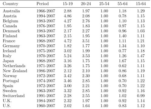
Table 2.1: Cyclical volatility of unemployment by age group, 20 OECD countries
Country Period 15-19 20-24 25-54 55-64 15-64
Australia 1966-2007 2.88 1.97 1.00 1.18 1.29
Austria 1994-2007 4.86 2.08 1.00 0.78 1.15
Belgium 1983-2007 4.27 2.76 1.00 1.10 1.13
Canada 1976-2007 1.95 1.83 1.00 0.97 1.15
Denmark 1983-2007 2.17 2.27 1.00 0.96 1.03
Finland 1963-2007 2.15 1.95 1.00 1.40 1.11
France 1968-2007 4.72 3.51 1.00 1.11 1.21
Germany 1970-2007 1.82 1.77 1.00 1.34 1.10
Ireland 1975-2007 3.02 1.99 1.00 0.77 1.18
Italy 1970-2007 5.24 3.53 1.00 1.26 1.47
Japan 1968-2007 3.16 1.75 1.00 1.67 1.15
Netherlands 1971-2007 3.26 1.75 1.00 0.62 1.11
New Zealand 1986-2007 2.12 2.10 1.00 0.86 1.19
Norway 1972-2007 3.42 2.30 1.00 0.68 1.11
Portugal 1974-2007 3.46 2.85 1.00 0.70 1.22
Spain 1972-2007 3.00 2.21 1.00 0.70 1.22
Sweden 1963-2007 3.32 2.85 1.00 0.92 1.16
Switzerland 1991-2007 2.28 2.55 1.00 1.02 0.99
U.K. 1984-2007 2.32 1.97 1.00 0.92 1.14
U.S. 1960-2007 2.02 1.64 1.00 0.83 1.12
Notes: Cyclical volatility of the unemployment rate is filtered by a one-sided HP filter with a smoothing parameter of 100. It is expressed relative to the prime-age (25-54).
trend reverses in several countries17when it comes to old workers. Among these, the unemployment volatility of old workers is relatively high for Japan, Germany, and Finland, which are currently facing serious aging of the labor force18. I also report aggregate unemployment volatility (15-64) in the last column, which is higher than that of prime-age workers for almost all 20 countries19because of the
17Which include Australia, Belgium, Finland, France, Germany, Italy, Japan, and Switzerland.
18The labor force share of the old (55-64) for these three countries in 2015 are, respec- tively, 19.91%, 18.71%, and 18.37%, ranking top 3 among the 20 OECD countries.
19Again, the exception is Switzerland. The aggregate unemployment volatility is lower than all age-specific volatilities. The reason for this puzzling observation could be due to the negative relation between age-specific unemployment rates. As the aggregate unem- ployment rate can be expressed as the average of age-specific unemployment rates weighted by the corresponding labor force share. Therefore, the aggregate unemployment volatility is composed of the volatility ofuitsitand the covariance of uitsitand ujtsjt, whereiandj
2.3. UNEMPLOYMENT VOLATILITY BY AGE 15 volatile behavior of young workers. In summary, the unemployment volatility of young workers is significantly higher than that of other age groups.
0 1 2 3
1960 1965 1970 1975 1980 1985 1990 1995 2000 2005
Time-varying Volatility
U.S.
Young Prime-age Old
0 1 2 3
1976 1981 1986 1991 1996 2001 2006
Canada
0 1 2 3
1984 1989 1994 1999 2004
Time-varying Volatility
Year U.K.
0 1 2 3
1970 1975 1980 1985 1990 1995 2000 2005
Year Germany
Figure 2.1: Time-varying unemployment volatility by age group Notes: Solid line is for young workers (15-24); dotted, triangle-hatched line is for prime-age workers (25-54); and solid, square-hatched line is for old workers (55-64).
The aforementioned measure is straightforward and easy to compare across age groups, but as summary statistics, it could lead to misleading interpretation.
One might wonder whether the observed pattern is a persistent demographic feature or is simply due to temporary shocks. For example, right before the
are the indexes for different age groups. If the unemployment rates of young workers and the prime-age move in opposite direction, suppose that it is due to certain labor market institutions which only favor the job finding probability of young workers, we will see a negative covariance ofuYtsYt and uPt sPt . And summation of these terms gives a lower value for aggregate unemployment volatility. This is also one of the reasons that I add labor market institutions into the analysis.
beginning of 2005, there was a big spike in the unemployment rate of the age group of 60-64 years in Germany. The reason is that January 1, 2005 marked the effective date of the Hartz IV reform, which shortened the duration and lowered the level of unemployment benefits. This creates an incentive for old workers to enter the unemployment pool and grab the last chance for high unemployment benefit without having much to lose. Potentially, this could be the reason for the higher unemployment volatility of old workers compared to that of prime-age workers for Germany as shown in Table 2.1, rather than any essential difference among workers of different ages. A similar logic also applies to the high values for young workers, which might be the result of changes in certain labor market institutions that only impact young workers. Therefore, it is also necessary to ascertain the time-varying measure of unemployment volatility.
Figure 2.1 shows the volatility measure based on SV with AR by age group for four countries. It displays distinctive features. For the U.S. and Canada, the unemployment volatility of young workers (solid line) is obviously above the values for prime-age (dotted and triangle-hatched line) and old workers (solid and square-hatched line). The value for prime-age workers is slightly higher than that for old workers over most of the time for the U.S., while the two almost coincide for Canada. For the U.K. and Germany, the value for old workers even overtakes that for young workers. For the U.K., this happens only once; while for Germany, though, this lasts for about two decades. Besides, we see there is indeed a sudden spike around 2005 in the unemployment volatility of old workers in Germany, but its long-lasting high value does not seem to be driven by the labor market reform in 2005.
Based on the examination of the time-varying unemployment volatilities by age group also for the other 16 countries20, I conclude that the unemployment volatility of young workers is the highest in general, and this is more likely to be a persistent demographic feature over time. The value for old workers frequently overtakes that for prime-age workers for a few countries (Japan, Germany, and Finland), but overall these two are quite close.
20See Appendix A.4 for the measures of other sixteen countries.
2.4. EMPIRICAL IDENTIFICATION 17
2.4 Empirical identification of the role of demographic changes
In this section, I employ the panel data model to study the relationship between unemployment volatility and demographic changes in the 20 OECD countries.
For age-specific unemployment volatility, I find the following: (1) the variation in the youth share has a quantitatively large and statistically significantly positive effect on the unemployment volatility ofyoung workers, and (2) no statistically significant relationship is detected among prime-age and old workers. After the spillover effect is identified, I go on to check for aggregate unemployment volatility and find that the variation in the youth share also has a statistically significant effect onaggregate unemployment volatility.
2.4.1 Unemployment volatility of young workers
In this subsection, I first present a brief look at the comovement between the unemployment volatility of young workers and the youth share. I then check the time series properties of these two series, and finally report the regression results.
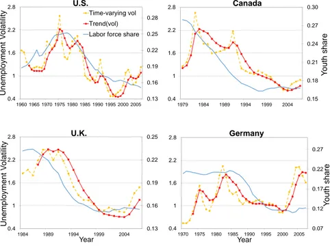
Figure 2.2 presents the time series of the time-varying unemployment volatil- ity of young workers and the youth share for the U.S., U.K., Canada, and Ger- many. In the U.S., the cyclical behavior can be divided into two distinct periods, one with a persistent rise from 1960s to the mid-1970s, and the other with a de- cline from the mid-1970s. Coincidentally, the evolution of the youth share can also be characterized by a similar pattern—a rise with the entry of baby boomers into the workforce in the 1960s and the 1970s, and then a decline from the late 1970s. In Canada and the U.K., both series share a monotonically decreasing trend over time. For Germany, both series share a common decline from the mid-1980s to the early 2000s.
0.13 0.16 0.19 0.22 0.25 0.28
0.4 1 1.6 2.2 2.8
1960 1965 1970 1975 1980 1985 1990 1995 2000 2005
Unemployment Volatility
U.S.
Time-varying vol Trend(vol) Labor force share
0.15 0.18 0.21 0.24 0.27 0.30
0.4 1 1.6 2.2 2.8
1979 1984 1989 1994 1999 2004
Youth share
Canada
0.13 0.16 0.19 0.22 0.25
0.4 1 1.6 2.2 2.8
1984 1989 1994 1999 2004
Unemployment Volatility
Year U.K.
0.07 0.12 0.17 0.22 0.27
0.4 1 1.6 2.2 2.8
1970 1975 1980 1985 1990 1995 2000 2005
Youth share
Year Germany
Figure 2.2: Youth share and unemployment volatility of young workers Notes: Solid line is the youth share; dotted, circle-hatched line is the
time-varying unemployment volatility of young workers; solid, square-hatched line is the trend of unemployment volatility which is filtered using a one-sided HP filter with a smoothing parameter of 100.
2.4.1.1 Time series properties
Before moving to regression analysis, it is necessary to check whether unemploy- ment volatility is intrinsically driven by demographic changes or only coinciden- tally shares a similar trend. This concern comes from the insufficient variation in both series21. The rather monotonous variation could arouse the suspicion of spurious regression.
21Due to the long-term decline in birth rate and increase in life expectancy, the youth share decreases persistently from the 1980s, at the same time, there is also a decline in the unemployment volatility of the young in most OECD countries.
2.4. EMPIRICAL IDENTIFICATION 19 To take care of this, I first check the stationarity of the relevant series. The upper part of Table 2.2 reports the results of panel unit root tests of the youth share and the unemployment volatility of young workers. For the youth share, after projecting out fixed effects (FE), I show that the null hypothesis of a unit root is rejected as a panel by the Maddala and Wu (1999) test (MW)22, and it is rejected at 5 percent level of significance in six countries (out of 20) by country- specific augmented Dickey and Fuller (1979) tests (ADF). For unemployment volatility of young workers, after projecting out fixed effects and time effects (FETE), along with the effects of labor market institutions (LMIs) and external shock23, the null hypothesis is rejected at 1 percent level of significance by the MW test as a panel. Besides, it is rejected in six countries by country-specific tests. These suggest the two series are more likely to be stationary.
However, I also detect cross-sectional dependence in the data. Columns 1 and 2 in the middle part show that, although the values for the average cross-sectional correlation ¯ρare low, the Pesaran (2004) cross-sectional dependence (CD) tests are significant. This strongly suggests the existence of cross-sectional dependence in both series. As the panel unit root tests are biased toward stationarity when cross-sectional dependence is neglected according to O’Connell (1998), we cannot fully rule out non-stationarity. In Column 3, I also carry out the same test for unemployment volatility by projecting out only fixed effects and time effects.
The results are similar. The reason for this exercise is to show that, with a model setup similar to Jaimovich and Siu (2009), cross-sectional dependence is likely to be a potential reason for biased estimates.
Therefore, I also carry out cointegration tests as shown in the lower part of Table 2.2. Even if these two series were non-stationary, panel regression is still capable of detecting the true relationship if they are cointegrated24. Technically, if panel cointegration tests reject the null hypothesis of a unit root in the error terms of the regressions, the panel regressions still offer meaningful results even with the presence of cross-sectional dependence. The results show that there
22It combines the p-values of the country-specific ADF tests.
23I use a fixed effect model and regress the unemployment volatility of each country on time dummies, the corresponding labor market institution indicators, and an external demand shock. Then, I use the residuals to calculate the country-specific unit root tests.
24Phillips and Moon (1999) show that a consistent estimation can also be obtained with neither stationarity nor cointegration, but their result relies on cross-sectional indepen- dence.
is indeed a cointegrating relationship between the youth share and the unem- ployment volatility of young workers, both shown by the cointegration tests as a panel and the ADF tests of individual countries.25
Table 2.2: Specification tests
Model FE FETE+LMIs FETE
(1) (2) (3)
Variable youth share unem. vol. unem. vol.
(young) (young)
ADF unit root tests of the series Panel unit root
test
73.74 83.81 91.74
P-value [0.00] [0.00] [0.00]
#pi65% 6/20 6/20 7/20
Cross-sectional dependence Average
correlation
0.04 -0.03 -0.03
CD test 3.24 -2.37 -2.09
P-value [0.00] [0.02] [0.04]
Panel cointegration test Panel unit root
test
- 87.47 93.02
P-value - [0.00] [0.00]
#pi65% - 7/20 7/20
Notes: Sample period: 1960-2007, unbalanced panel of 20 OECD countries.
FE refers to a model which projects out fixed effects; FETE refers to a model which projects out both fixed effects and time effects; FETE + LMIs refers to a model which not only projects out fixed effects and time effects but also excludes the effects from labor market institutions and external demand shock.
CD test refers to cross-sectional dependence test. Details for the calculation of test statistics can be found in Appendix A.5.
25I regressσYit−σ¯Yit on the regressors, which includessYit−s¯Yit , time dummies, labor market indicators, an external demand shock, and a constant term for each country. Then, I carry out the country-specific ADF tests on the error terms and count the number of countries with a p-value lower than 5%. The panel cointegration tests are constructed similarly as the panel unit root tests in the top left of Table 2.2, by combining the p-values from the country-specific ADF tests.
2.4. EMPIRICAL IDENTIFICATION 21 2.4.1.2 Regression results
The regression setup is a panel data model with fixed effects and time effects (FETE):
σit=αi+βt+γsit+λXit+εit, (2.3) whereσitis the volatility measure based on SV with AR for countryiat timet;
sit is the share of the corresponding age group in the labor force;Xit includes the five indicators of the labor market institutions and the external shock as mentioned;αiis a country fixed effect; andβtdenotes a full set of time dummies to control for time effects.
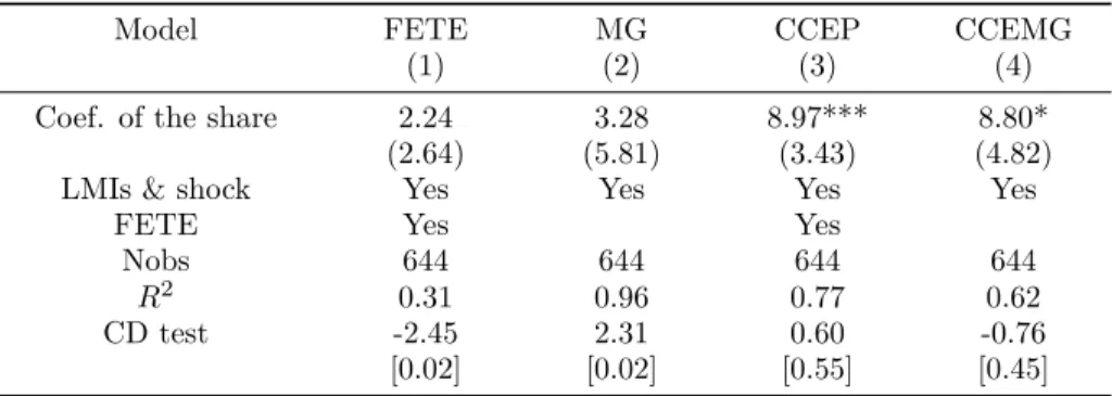
Table 2.3: Unemployment volatility and the share of labor force: young workers
Model FETE
(1)
MG (2)
CCEP (3)
CCEMG (4) Coef. of the share 2.24
(2.64)
3.28 (5.81)
8.97***
(3.43)
8.80*
(4.82)
LMIs & shock Yes Yes Yes Yes
FETE Yes Yes
Nobs 644 644 644 644
R2 0.31 0.96 0.77 0.62
CD test -2.45
[0.02]
2.31 [0.02]
0.60 [0.55]
-0.76 [0.45]
Notes: Sample period: 1960-2007, unbalanced panel of 20 OECD countries. The dependent variable is the unemployment volatility of young workers.
All models exclude the effects of labor market institutions and external demand shock. FETE refers to a model which also projects out fixed effect and time effects; MG refers to mean group estimator with trends; CCEP refers to a model that projects out fixed effects and excludes the effects of the unobserved common factors; and CCEMG refers to the mean group model, which also excludes the effects of the unobserved common factors.
Driscoll-Kraay standard errors for Columns 1 and 2 and Newey-West standard errors for Columns 3 and 4 are in parentheses. p values are in square brackets.
*** and * stand for significance levels of 1% and 10%, respectively.
Table 2.3 presents the regression results for young workers. Columns 1 and 2 give the results of fixed effects and time effects (FETE) and the mean group (MG) estimations. With both estimators reported, we can reduce the risk of
model misspecification26. I also include a trend component in the MG estimator, as there appears to be a trend in the unemployment volatility of young workers for some countries. Besides, I report the Driscoll and Kraay (1998)27 standard error for both, which is robust to the missing of unobserved common factors unrelated to regressors. The results in the first row show that the coefficients are both positive but insignificant. It seems that the youth share does not have any statistically significant impact on the unemployment volatility of young workers. At the same time, though, I detect cross-sectional dependence, which suggests that the unobserved common factors in the error term is correlated with regressors. In this case, both FETE and MG estimators are biased. Still the former is used as the main estimator in Jaimovich and Siu (2009).
To deal with this problem, I follow the approach proposed by Pesaran (2006) with common correlated effects (CCE) estimators28. Here, the unobserved com- mon factors are proxied by the cross-sectional averages of all observed variables, including both the dependent variable and the regressors. As a result, the unob- served common factors are eliminated and the consistency of panel estimator is ensured. Column 3 reports the pooled common correlated effect (CCEP) estima- tor, the fixed-effect version of the CCE estimator. Now, the coefficient becomes significant at the 1 percent level, meaning the youth share has a positive im- pact on the unemployment volatility of young workers29. The magnitude of the
26The FETE estimator pools the data together and assumes that the slope coefficients, the intercepts, and error variances of different age groups are all identical. Thus it may produce inconsistent estimates in case of heterogeneity among age groups. While the MG estimator by Pesaran and Smith (1995) fits the model separately for each group, therefore the estimated parameters are allowed to be heterogeneous across groups.
27Driscoll and Kraay (1998) propose a non-parametric covariance matrix estimator for the consistent standard errors. They use the cross-sectional average of the orthogonality moments of the product of the regressors and the residual to act as a Newey-West type weight in the estimation.
28Other approaches include the seemingly unrelated regressions (SUR) approach and the principal components approach. Among all, the CCE estimator is the most attractive because of its simplicity. One only needs to add the cross-sectional averages of observed variables in the fixed effects panel estimation and corrects the standard errors accordingly.
29Meanwhile, I also report the CCEP estimators of the coefficients of labor market institutions in Appendix A.6. Of which, the coefficients of union density and employment protection legislation are sizable and statistically significant. The effect of union density on unemployment volatility is positive, because union density is positively related to real wage rigidities and firms have to cut employees in case of recession; while the effect of employment protection legislation is negative, which is consistent with the finding of Blanchard and Portugal (2001).
2.4. EMPIRICAL IDENTIFICATION 23 coefficient suggests that a 10% increase in the youth share would increase the un- employment volatility of young workers by almost 0.90. Since the time-varying measure of the unemployment volatility of young workers for the U.S. is 2.57 in 1975 and 0.46 in 1995, the regression result suggests that: If there were a decline of 23.5% less young workers in the labor force over these 12 years, and all other conditions unchanged, then we would have the same decline in unemployment volatility of young workers. In other words, the actual decline in the youth share is 8.2%, meaning demographic changes account for approximately a third of the variation of the unemployment volatility of young workers.
To further check the robustness of the results and allow for more flexibility in the model setup, I also report the results of the common correlated effects mean group (CCEMG) estimator in Column 4, the mean group version of the CCE estimator. It allows for heterogeneous slope coefficients and also controls for cross-sectional dependence. The results confirm the positive impact of the youth share on unemployment volatility as implied by the CCEP estimator. The magnitude of the coefficient is slightly lower and less significant. Considering that the country-specific coefficients are relaxed to be heterogeneous, one should expect a lower significance level. The null assumption of cross-sectional inde- pendence cannot be rejected either, which ensures the validity of the estimation result.
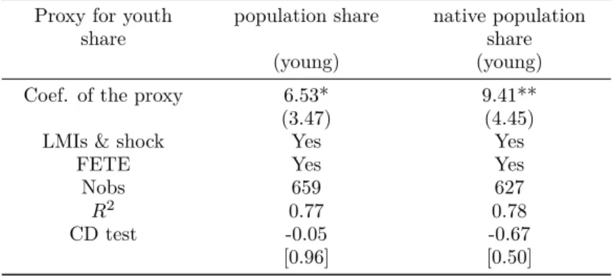
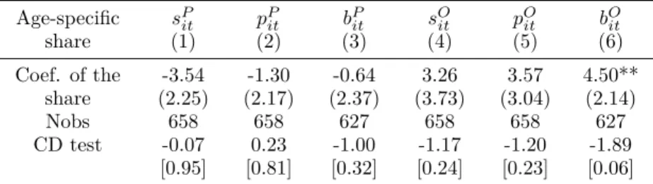
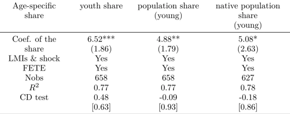
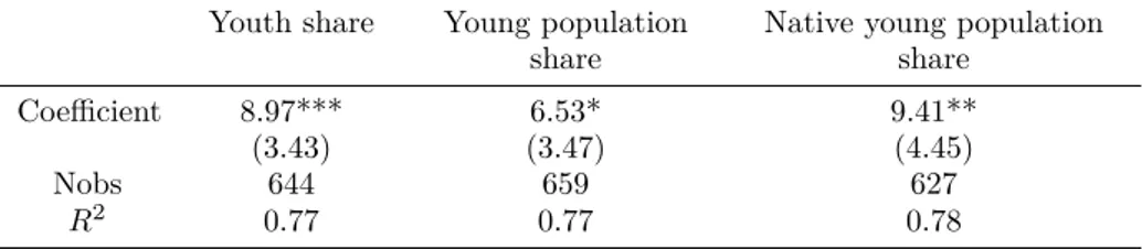
As the youth share also depends on the participation rate of young workers, its validity as a measure of demographics lies in the exogeneity condition that the participation rate of young workers plays a minor role in the unemployment dynamics of young workers. To verify this, I use the share of young population as a proxy for the youth share. As the share of young population is independent of their labor force participation decision, the endogeneity bias is likely to be excluded. Column 1 of Table 2.4 reports the results of CCEP estimation result.
The coefficient is positive and significant at the 10% level. Moreover, the level of the coefficient is similar to that in Table 2.3. The CD test also suggests that cross-sectional dependence is well taken care of by the CCEP estimator.
Table 2.4: Labor force participation and international migration: further robust check
Proxy for youth share
population share native population share
(young) (young)
Coef. of the proxy 6.53*
(3.47)
9.41**
(4.45)
LMIs & shock Yes Yes
FETE Yes Yes
Nobs 659 627
R2 0.77 0.78
CD test -0.05
[0.96]
-0.67 [0.50]
Notes: Unbalanced panel of 20 OECD countries, sample period: 1960-2007 for Column 1 and 1970-2007 for Column 2. The dependent variable is the unemployment volatility of young workers.
Model used in this table is the pooled common correlated effect (CCEP)
estimator. Newey-West standard errors are in parentheses. p values are in square brackets. ** and * stand for significance levels of 1% and 5%, respectively.
However, if the response of the labor market activity of a foreign young worker to shocks differs from the response of that of a native young worker, the young population share is still likely to be endogenous as international migration decision is unaccounted for. To take care of this, Jaimovich and Siu (2009) suggest using the share of the native population30. As the historical data of this distribution are directly unavailable, they proxy it by the projection of the labor force share on the lagged birth rates. Instead, I use directly the age distribution of native population calculated from data on lagged birth rates and population size. With historical data on birth rates and population from Mitchell (2008) and Maddison (2003), I first get the historical series of the size of newborns.
Since the population size of the young native population today is just the sum of newborns 15 to 24 years ago, I calculate the share of native young population as
bYit= Pj=24
j=15bi,t−jpi,t−j
Pj=64
j=15bi,t−jpi,t−j
, (2.4)
30Since the past fertility decision is made long before the realization of shocks affecting the current unemployment volatility, the distribution of native young population is not likely to be influenced by international migration.