IHS Economics Series Working Paper 318
November 2015
The structure of labor market flows
Tamás K. Papp
Impressum Author(s):
Tamás K. Papp Title:
The structure of labor market flows ISSN: Unspecified
2015 Institut für Höhere Studien - Institute for Advanced Studies (IHS) Josefstädter Straße 39, A-1080 Wien
E-Mail: o ce@ihs.ac.atffi Web: ww w .ihs.ac. a t
All IHS Working Papers are available online: http://irihs. ihs. ac.at/view/ihs_series/
This paper is available for download without charge at:
https://irihs.ihs.ac.at/id/eprint/3794/
The structure of labor market flows
∗Tam ´as K. Papp†
Institute for Advanced Studies, Vienna
November 12, 2015
Abstract
We show that a general class of frictional labor market models with a participation margin and an individual-specific state can only match labor market transition rates within a certain range, which we characterize analytically. Transition rates in the data are outside the range the model can match, which explains the failure of previous papers to calibrate to these flows. We also exam- ine whether extending the model can bring it closer to the data, and find that endogenous search intensity and state-dependent separation rates do not help, but misclassification, persistently inac- tive workers, and modifications of the productivity process such as learning on the job can match the gross flows.
Graphical abstract
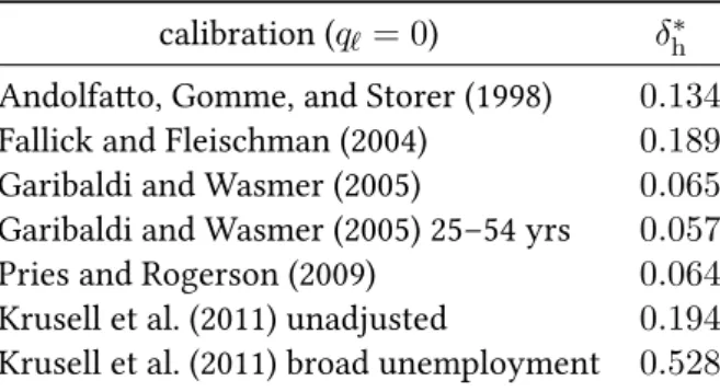
share of separations to inactivity (+: data, lines: model) Krusell et al. (2011), broad unemployment
Krusell et al. (2011), unadjusted Pries and Rogerson (2009) Garibaldi and Wasmer (2005), 25−54 yrs Garibaldi and Wasmer (2005), 15−64 yrs Fallick and Fleischman (2004) Andolfatto, Gomme, and Storer (1998)
0.2 0.4 0.6 0.8
+ + + +
+ + +
∗I thank Victor Dorofeenko for research assistance. I am grateful for the comments from ´Arp ´ad ´Abrah ´am, Larry Blume, Tobias Broer, Melvyn Coles, Mike Elsby, Wouter den Haan, Christian Haefke, Pietro Garibaldi, Nezih Guner, Per Krusell, Thomas Lubik, Pedro Maia Gomes, Monika Gehrig-Merz, Rachel Ngai, Fabien Postel-Vinay, Michael Reiter, Etienne Wasmer, and participants at the VGSE Macro Research Seminar, Search and Matching 2014 meeting in Edinburgh, ESSIM 2015 in Tarragona, and the conference in honor of Christopher A. Pissarides at Sciences Po in 2015. I acknowledge support from the Jubil¨aumsfonds grant (16256) of the Austrian National Bank.
†
tpapp@ihs.ac.at
1 Introduction
The last ten years have seen the emergence of comprehensive models for the labor market, which aim to explain the individual-level dynamics of both labor supply choices and unemployment, modeling transitions between employment, unemployment, and non-participation in a frictional labor market.
Recent examples are Garibaldi and Wasmer (2005) and Krusell et al. (2011): the most important addition to the previous literature is that these papers aim to pin down and explain not only stocks, but also gross labor market flows. These flows are very important for policy analysis: to the extent that they are exogenous from the perspective of an individual, such as exogenous separations, they are usually insurable to a very limited extent (if at all), and when they are the outcome of optimizing behavior, such as participation decisions, it is important to understand how they would responds to various policy measures, for example taxation and unemployment insurance.
Both Garibaldi and Wasmer (2005) and Krusell et al. (2011) calibrate to the observed labor market flows, and are able to explain them with a seemingly small discrepancy between the implications of the model and the data. This paper demonstrates that this small discrepancy is significant, and it is not something that can be improved on with a more careful calibration: a general class of simple labor market models with labor market frictions, and an individual-specific state which drives participation decisions and evolves stochastically, can only explain labor market transition rates if they are within a certain range. Examination of the data used by various papers shows that the flows are outside the range that the model can explain. Consequently, the inability of this model family to match the data stems not from the lack of enough free variables, but is a feature ofboththe model and the data: as we explain below, matching certain flows constrain the ability of the model to match other flows, and in the data the latter flows are outside the admissible range of the model.
To make things concrete, let E, U, and I denote employment, unemployment, and inactivity (non- participation),1respectively, andλUI, λUE, . . . denote continuous-time transition rates between these states. The central question of this paper is the following: for a given model and 6-tuple of transition rates
Λ = (λUI, λIU, λIE, λUE, λEI, λEU), can we find a parameterization of the model that generatesΛ?
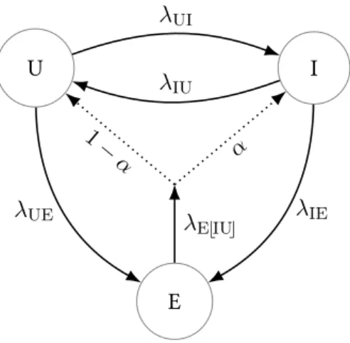
The key contribution of this paper is an analytical characterization of this question for various models, and the introduction of a particular way of calibrating to flows that allows a tractable anal- ysis of this nonlinear problem. Figure 1 provides a stylized summary of the way we characterize the calibration of the models we examine. First, we calibrate to the flows between unemployment and inactivity,λIUandλUI, thetotalflows out of employment
λE⌊IU⌋=λEI+λEU,
and the job finding ratesλIEandλUE. This way we match five out of the six moments we target. Then
1In this paper we refer to non-participants asinactives, because we want to avoid confusion with the non-employed in the notation in Section 2.
we examine the ratio
α= λIE
λE⌊IU⌋
(1) as a function of the free parameters of the model, and see whether the range ofα— which is, of course, a function of the other five moments we have matched — contains its counterpart in the data. If it does, then we say that a particular set of flowsΛareadmissiblefor a given model.
E
U I
λUI
λIU
λUE λIE
1− α α
λE⌊IU⌋
Figure 1: Calibration of labor market transition rates. We calibrate toλIU,λUI,λE⌊IU⌋ =λEI+λEU, λUE, andλIE(solid lines). Then we characterize the fractionα=λEI/λE⌊IU⌋(dotted lines).
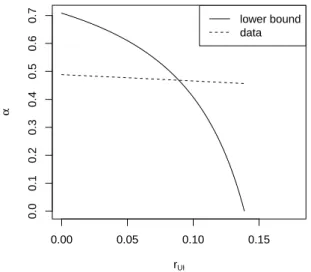
For some of the models we examine, including the benchmark model of Section 2 which nests Garibaldi and Wasmer (2005) and closely approximates a special case of Krusell et al. (2011), we find that when calibrating to the other five moments, there is a lower boundα∗ such that a particularαis admissible if and only if
α∗≤α≤1,
where we characterize the lower boundα∗ analytically as a function of the five other moments we calibrate to.
We briefly summarize the benchmark model and explain the intuition behind this result. The bench- mark model of Section 2 is in continuous time with linear utility, the only state of a worker is individual- specific, and it determines wages and the flow utility of non-employment (eg the value of leisure, home production, and unemployment benefits). The difference of the two is the flow surplus, and it plays a key role in the labor market participation choice. Exogenous events, which can be thought of as stylized representations of shocks that change either wages or the value of non-employment, change the individual’s state and thus the flow surplus. Employed workers experience exogenous separations, but may also separate endogenously after if their state and consequently their flow surplus changes.
Non-employed workers can choose to searchactivelyorpassively. Job opportunities arrive exoge- nously, and are either accepted or rejected by the worker, and active search results in a higher arrival rate, but entails a flow cost. Consequently, the flow surplus partitions the state space of non-employed workers into three regions: those with a high surplus for whom it is worthwhile to pay the search cost in exchange for a higher arrival rate of job offers, so they search actively (H), those who would accept a job but would not pay the search cost, and they search passively (M), and those whose flow surplus
is so low that they would never accept a job (L).
We identify unemployed workers in H with active search, and the other two regions L andM with non-participation. A key feature of the model is that the five flows we calibrate to constrain the calibration of the stochastic process for the individual-specific state, which in turn determines the distribution ofemployedworkers in regionsMandHof the parameter space, which we callmarginal and non-marginal workers, respectively. This is important because after an exogenous separation, non-marginal workers search actively, while marginal workers search passively, and this constrains the share ofλEIandλEUflows inλE⌊IU⌋, thus determiningαin (1).
Looking at the data in various papers that calibrate to labor market flows in Section 3, we find that αdata< α∗,
in other words when calibrating to the other five moments,αin the data is lower than the lower bound of what the model can be calibrated to and thus the flows are not admissible in the benchmark model.
Mostly, this happens because in the data,
λIU+λE⌊IU⌋≪λUI,
or in other words, having so many inactives relative to the unemployed requires that UI transition rates are much larger than IU rates. In theory, a large separation rate from E could alleviate this, because, sinceλIE < λUE, it would lead to relatively fewer marginal inactives; but of course this is not a feature of the data. We show that this discrepancy cannot be explained by small sample size, and it holds for all papers we have examined, which suggests that a crucial ingredient is missing from our models if we want to calibrate to labor market flows.
Consequently, Section 4 examines various extensions to the benchmark model. First, recognizing that the simple binary search technology in the benchmark model may be too restrictive, in Section 4.1 we endogenize search effort with a continuous variable, and show that no matter where we draw the line between inactivity and unemployment, the flows can be mapped to those of the benchmark model, and this extension does not improve its ability to match the data.
In Section 4.2 we extend the model with state-dependent separation rates: allowing for the possibil- ity that marginal workers experience higher rates of exogenous separation compared to non-marginal workers. We think of this extension as reduced form for a model with firm- or match-specific pro- ductivity, with the idea that marginal matches are more fragile. Since this modification increasesλEI flows, it actually increasesα∗, moving the model further away from the data.
A crucial assumption in the result about the benchmark model is that we impose a stochastic process for the individual-specific state that is independent of the labor market status, which makes λIUandλUIrates, which are from the observation of the non-employed, constrain the share of marginal employed. Breaking the connection between the stochastic processes for the individual-specific state for the employed and non-employed could in principle alleviate the problem of the benchmark model.
We show that this is indeed the case, first by examining a stylized model with permanently inactive workers in Section 4.3, then by introducing learning on the job in Section 4.4. Having permanently
inactive workers who never participate in labor market flows helps because we can assume that the λIU flows we observe are the weighed average of the same flows for permanently inactive workers (for whom it is zero) and the rest of the population, for whom they are consequently larger, and larger λIUflows would lowerα∗. In contrast, learning on the job works by decreasing the share of marginal employed, since by moving to a state with higher surplus they become non-marginal. We show that in theory both approaches can driveα∗ to0, and thus all possible flowsΛbecome admissible under either model.
Finally, in Section 4.5 we consider classification error, by allowing for the possibility that inactive or unemployed workers are misclassified into the other state in surveys, thus generating spurious flows.
We introduce a general theoretical framework for calculations with such processes, which provides a mapping from observed to underlying flows in a self-consistent way. We find misclassification of inactives as unemployedincreasesthe lower boundα∗, but misclassification of unemployed as inactive decreases α∗ and brings the model closer to the data — in fact, a UI misclassification probability for each observation around9%can bringα∗toαdata.
Our analysis is related to the various approaches in the literature that aim to explain participation and unemployment. As noted by Krusell et al. (2011), historically, frictionless versions of the standard growth model were mainly used to explain participation, mapping it to a choice on the labor/leisure margin: for example Hansen (1985) and Rogerson (1988), while models in the Diamond-Mortensen- Pissarides model family2have been used to explain unemployment with labor market frictions and the response of unemployment to aggregate fluctuations.3However, recognizing that satisfactory models should account for both unemployment and the participation margin, many papers incorporated the latter into frictional models of the labor market. Ljungqvist and Sargent (1998), Ljungqvist and Sargent (2007a), Alvarez and Veracierto (2000), and Veracierto (2008) are models that are similar to the one discussed in this paper along many dimensions, but they do not attempt to account for labor market flows across the three states. Coming from the other direction, Merz (1995), Andolfatto (1996), Gomes, Greenwood, and Rebelo (2001) include labor market frictions in the standard growth model, but do not distinguish unemployment and inactivity.
The two papers most closely related to this one are Garibaldi and Wasmer (2005) and Krusell et al.
(2011). In particular, our model nests the structure of Garibaldi and Wasmer (2005), formalizing the reason for the discrepancy between observed and generated flows in their paper in a more general setting. What we call marginal workers they term “employment hoarding”, since it results from the irreversibility of separations. Krusell et al. (2011) also focus on the flows, in a model that is essentially similar to ours except for the fact that they also allow risk aversion and saving. However, as noted in their paper, this does not have a significant effect on the flows, and thus would only complicate our analysis. Krusell et al. (2011) also argue that marginally inactive in the data should be counted as unemployed when accounting for the flows. However, this turns out to increase UI transition rates, increasing the distance between the model and the data even further. Both papers note the discrepancy between calibrated transition rates and the data, but focus on its consequences on the UI and IU flows.
In contrast to most of the literature, the models in this paper are very stylized, and we focus on
2See Pissarides (2000) for an introductory overview.
3
See, for example, Haan, Ramey, and Watson (2000), Costain and Reiter (2008), Shimer (2005).
discussing the theoretical properties of models, with respect to their ability to match labor market flows. This is necessary because in order to say that a particular set of flowsΛisnot admissible for a certain model, we need to be able to characterize the whole range of flows that are possible, which necessitates a stylized structure. The stylized models in this paper may not be directly applicable for policy questions, but are intended to serve as a useful guide on what to incorporate into models which are calibrated to labor market flows. This approach of characterizing the distance between data and models with a single scalar, and focusing on simple models to explore extensions that alleviate a puzzle was inspired by Hornstein, Krusell, and Violante (2011).
Also, this paper does not discuss the implications of the models for wages: the models are used to put structure on the observed transition rates between employment, unemployment and inactivity.
This is not because we think that wages are not important, but because explaining flows themselves appears to be difficult enough — also, since only the difference of wages and non-employment utility matters for the labor market flows in the models we discuss, strong assumptions on wage processes would be needed to connect wages and labor market flows. We leave incorporating wages for future research.
Most of the results in the paper are analytical, but illustrated with calculations using empirical data.
However, in order to avoid making the paper unreadable, we relegated most steps in the analytical proofs to the appendix, and only included important equations and simplified derivations in the main text. All analytical proofs and calculations have been checked using the symbolic algebra software Maxima (2014) and are available in the online Appendix A.
2 The benchmark model
In this section we introduce a model that serves as a starting point for the discussion of gross labor market transition rates. This model makes a compromise between tractability and generality: it is sim- ple enough to allow an analytical characterization of the results, yet at the same time general enough to nest or approximate partial equilibrium features of models in the literature; in particular, the model nests the partial equilibrium features of Garibaldi and Wasmer (2005). The model could be embedded in a general equilibrium framework, for example similarly to Hornstein, Krusell, and Violante (2011, Section 1.B), but this would not add to the key results of the paper.4
2.1 Preferences and technology
Time is continuous, workers are risk-neutral, ex-ante homogeneous and discount at rater.5We char- acterize the steady state equilibrium in which job offer rates are exogenous, conditional on search intensity. Workers are eitheremployed ornon-employed, and workers in the latter are categorized as eitherunemployedorinactive based on search activity. Since the model needs to be able to generate
4A general equilibrium formulation with job (vacancy) creation would just provide additional restrictions on the gross flows that the model can generate, and thus the range of labor market flows generated by a partial equilibrium model is necessarily larger than it would be for general equilibrium one. Using the latter would just complicate the formulation and distract from Lemma 1. A partial equilibrium formulation also precludes discussion of aggregate fluctuations and policy experiments, but both of those directions are outside the scope of this paper.
5We refer to all agents as workers, regardless of their current employment status.
apparent flows from seemingly inactive workers (ie those workers who are neither employed nor un- employed, in the sense that they do not search actively) into employment, we assume that workers who choose not to search actively also receive job offers, albeit at a lower rate.6Specifically, there are two search technologies available to all non-employed workers:active search, which entails a flow cost cwith job offers arriving at rateφh, andpassive searchwhich requires no search effort (ie a cost of0), and makes job offers arrive at rateφm. Naturally,φm< φh. This is a very stylized specification as it only allows a binary choice for search effort, we generalize this in Section 4.1.
Workers have an individual-specific statexthat we think of as a proxy for market opportunities, family, health, and preference shocks. Krusell et al. (2008) show that it is difficult to generate gross labor market flows between inactivity and unemployment without these shocks even in a very rich model with precautionary savings, in the absence of the latter this process will be the only source of flows between unemployment and inactivity, and also, to a certain extent, from employment to non- employment. We think of changes inx as major life events that affect the difference between labor market productivity and the the opportunity cost of working, such as changes in personal relation- ships or family status, a major illness, and education opportunities and attainments. The individual’s statexdetermines wagesw(x) and the utility flow for the nonemployed,u(x), where the latter in- cludes unemployment benefits, home production, and the value of leisure. This implies that all worker heterogeneity in the benchmark model is individual-specific, and there are no match- or firm-specific sources of wage dispersion.7
The statexis constant until achange eventarrives, in which case it is redrawn from an IID distri- butionx ∼F. Change events arrive at rateγ, independently of other events and states, particularly labor market status. We think ofγ as being a relatively low number, because major changes in work- ers’ market productivity or outside options are expected to be rare. Hornstein, Krusell, and Violante (2011) refer to this kind of process as apersistent process, and it is commonly used to specify stochastic processes which exhibit some degree of persistence (and thus autocorrelation), yet at the same time allowing a simple characterization of steady state distributions and transition rates.
This specification is restrictive in two ways: it only allows IID distributions forxconditional on a change event, and it imposes the same process for both the employed and non-employed. It turns out that the latter has important implications for matching labor market flows, and we consider various generalizations in Sections 4.3 and 4.4.8 At the same time, the benchmark model allows an arbitrary space for the values ofx: discrete distributions, subsets ofRn, or even combinations of the two, as long as they capture all payoff-relevant information and new values are IID conditional on a change event.
Employed workers may separate endogenously whenever they prefer non-employment to employ- ment — this happens if they experience a change event that results in a draw ofxwhere the difference betweenw(x)andb(x) is low. In addition, employed workers are also subject to exogenous separa-
6
As we discuss in Section 3, even though a fraction of these transition can be explained by time aggregation (inactive workers becoming unemployed and then employed between two observations), this flow is too large in the data to be assumed away.
7The model in Section 4.2 can be considered a reduced-form version of extending the benchmark model with match- or firm-specific heterogeneity in a way that marginal matches would be less robust to shocks, resulting in higher exogenous separations.
8
A previous version of this paper also had a generalization to non-IID distributions forF, which is omitted because it does not add significantly to the results but greatly complicates derivations.
tion shocks at rateσ. We assume that the separation rate is uniform and thus independent of worker surplus and history, we generalize this in Section 4.2. Table 1 summarizes the notation for parameters and endogenous objects of the benchmark model.
parameters
x∈ X individual-specific state and set of possible states γ arrival rate of change events forx
F distribution of newx, conditional on a change event
w(x) wage when employed
b(x) flow value of non-employment (unemployment benefit, leisure, and home production) φm, φh arrival of job offers for passive and active search
c flow cost of active search σ rate of exogenous separation
equilibrium objects
W(x),N(x) present discounted value of employment, non-employment S(x) present discounted value of the worker’s surplus
L⊂ X low surplus: no active search, non-employment preferred M⊂ X marginal surplus: passive search, employment preferred H⊂ X high surplus: active search
qℓ, qm, qh continuous-time rate of transition to regionsL,M,H, respectively
λIU,λIE,. . . observed transition rates betweenInactivity,Unemployment, andEmployment λE⌊IU⌋ transition rate out of employment,λEI+λEU
ν share of marginal workers among the inactive µ share of marginal workers among the employed α share ofλEIinλE⌊IU⌋
Table 1: Notation for the benchmark model of Section 2. Notation recycled for extensions.
2.2 Value and policy functions
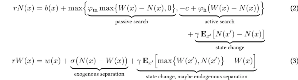
LetN(x)andW(x)denote the current present value of being non-employed or employed, respectively, with individual-specific statex. The continuous time Hamilton-Jacobi-Bellman equations are
rN(x) =b(x) + max {
φmmax{
W(x)−N(x),0}
passive search
,−c+φh(
W(x)−N(x))
active search
}
(2) +γEx′[
N(x′)−N(x)]
state change
rW(x) =w(x) +σ(
N(x)−W(x))
exogenous separation
+γEx′[ max{
W(x′), N(x′)}
−W(x)]
state change, maybe endogenous separation
(3)
Equation (2) states that a nonemployed worker receives benefits (which are function ofx), and can choose between passive and active search. For the former, offers are only accepted when working is preferable to non-employment, for the latter, the formulation above anticipates that when agents
choose to search actively, they accept the job they find. The exogenous state change always leaves a nonemployed worker nonemployed, and thus it generates flows between inactivity and unemploy- ment.
For an employed worker, (3) shows that the flow payoff is the wage, and the two possible transitions are exogenous separations and state changes. Exogenous separation always moves the worker into non-employment, while changes of the individual state can result in endogenous separation if the worker ends up in a state wherew(x)is low compared tob(x).
It can be shown that the system (2) and (3) has a unique solution using a standard contraction argument, consequently the model parameters determine the policy function for the binary search intensity. However, as usual in this model family, it is more convenient to analyze the model in terms of the worker’s surplus
S(x) =W(x)−N(x) Rewrite (2) and (3) in terms of the surplus as
rN(x) =b(x) + max(φmS(x)+, φhS(x)−c) +γ( Ex′[
N(x′)]
−N(x))
(4) rW(x) =w(x)−σS(x) +γ
( Ex′
[S(x′)+]
+γEx′
[N(x′)]
−W(x) )
(5) whereS(x)+= max(
0, S(x)) .
Introduce the flow surpluss(x) =w(x)−b(x), then combine (4) and (5) into (r+σ)S(x) =s(x)−max(φmS(x)+, φhS(x)−c)
opportunity cost of not searching
+γ( Ex′[
S(x′)+]
−S(x))
change event
(6)
Equation (6) characterizes the worker’s surplus in terms of the model parameters. The effective dis- count rate on the left hand side is the subjective discount raterand the exogenous separation rateσ, as exogenous separations terminate the match. On the right hand side, s(x) = w(x)−b(x) is the flow payment for a surplus: this demonstrates that only the difference of market productivity and the opportunity cost of working (such as the value of leisure, home production, or unemployment benefits) matters for the determination of the surplus and consequently the search policy; in this model, wages and flows are orthogonal features of the data, and information about one does not help in identifying the other without additional restrictions on processes. The second term on the right hand side is the opportunity cost of not searching, either actively or passively. The last term is for the changes in sur- plus: since the worker will terminate the match wheneverS(x′) < 0, the surplus cannot be below0 for a new drawx′.
WhenS(x) <0, the worker would not accept a job anyway, and thus defaults to passive search.
Otherwise, the worker compares the search costcto the gain from a higher job finding rate (φh− φm)S(x), and chooses active or passive search accordingly. Consequently, comparingc/(φh−φm) toS(x)partitionsX into three regions which characterize the policy function and are crucial for the
determination of flows:
L={
s:S(x)<0} M ={
s: 0≤S(x)< c/(φh−φm)} H={
s:c/(φh−φm)≤S(x)}
We choose these regions for mapping worker search behavior to the data. In regionL ⊂ X (low surplus), nonemployed workers do not search actively, and if they encounter a job, they choose to remain nonemployed because their surplus from the job would not be positive, while in regionM ⊂ X (middle ormarginal surplus), nonemployed workers still do not search actively because their surplus does not justify the cost, but would accept a job if they were offered one. We assume that survey data would record these workers asinactive, or out of the labor force. We call non-employed in regionM marginal inactives.
In the regionH⊂ X (high surplus), nonemployed workers search actively, and thus from now on we assume that they are recorded in survey data asunemployed. We useℓ,m, andhas subscripts for notation below, always referring to the respective region.
Even though only nonemployed workers have a nontrivial choice in this model, when we account for the distributions it is important to also distinguish employed workers based on the partition above.
Naturally, there are no employed workers inL, since employed workers ending up in this region after a change event always quit their job, separating endogenously. In contrast, employed workers ending up in regionMafter a change event do not quit, but they would not search actively if they experienced exogenous separation. For this reason, we call themmarginal employed.
2.3 Latent and observed flows
Let E, U, and I denote employment, unemployment, and inactivity (non-participation) in survey data.9 The state of a worker is(x,{employment,non-employment}), which is mapped to E, U, and I as dis- cussed above. LetλUI, λUE, . . . denote continuous-time transition rates from U to I, U to E, etc. We now map model parameters to observed flows.
Since only unemployed find jobs at rateφh, it is straightforward that
λUE=φh (7)
All inactive workers transition into regionHat the same rate λIU=γ
∫
x′∈H
dF(x′)≡qh (8)
where we have defined qh as the product of the arrival rate of the change event, multiplied by the probability thatx′ ∈H, since draws withx′∈L⊎Mwould not result in an observable transition from
9
Several papers use N for non-participation, in this paper we use I to avoid confusion with non-employment.
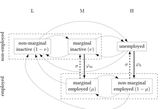
non-marginal inactive(1−ν)
marginal
inactive(ν) unemployed
marginal employed(µ)
non-marginal employed(1−µ)
L M H
employednon-employed
φm φh
σ σ
Figure 2: Latent and observed flows. Dotted arrows correspond changes inx. When these happen betweenLandMfor nonemployed workers (both of which are counted as inactive) orMandHfor employed workers, they are not observed as transitions in a dataset with three states, otherwise they show up as UI, IU, or EI transitions. Dashed arrows are exogenous separations (EI or EU, depending on whetherxis inMorH), while solid arrows correspond to job finding (IE or UE), similarly depending onx.
I to U. Similarly, defining qℓ≡γ
∫
x′∈L
dF(x′) and qm≡γ
∫
x′∈M
dF(x′) (9)
allows us to write
λUI=qℓ+qm. (10)
For the other three transitions — λIE, λEU, λEI — we have to keep track of the distribution of workers, but only with respect to the partitionX = L⊎M⊎H. This is because conditional on a change event, shocks toxare IID, and thus once we know that the worker is in a particular region of the state space, we know which observed transition to map to between E, U, and I. Overall, there are six possible combinations of(L,M,H)and employment status, but only five of them have any mass in the steady state since there are no employed workers inL.
For analytical convenience, we characterize this distribution with the totalof non-employed and employed workers in each regionmℓ, mm, mh, and the mass of employed workersem, eh, where the subscript refers to the region. Then the mass of marginal inactives ismm−em, and the mass if unem- ployed ismh−eh.
The steady state flow balance equations for the first three are
mℓ·(qm+qh) = (mm+mh)·qℓ (11) mm·(qℓ+qh) = (mℓ+mh)·qm (12) mh·(qℓ+qm) = (mℓ+mm)·qh (13)
mℓ+mm+mh = 1 (14)
In each equation, the left hand side shows the outflows, while the right hand side shows the inflows.
For example, in (11), workers transition fromLtoMandHwith ratesqmandqh, respectively, while workers flow intoLfrom both of the latter regions at rateqℓ. Because of symmetry, it is easy to see that the solution to the system (11)–(14) is
mℓ = qℓ
qℓ+qm+qh mm= qm
qℓ+qm+qh mh= qh qℓ+qm+qh Foremandeh, the steady state flow balance equations are
em·(qℓ+qh+σ) =eh·qm+ (mm−em)·φm (15) eh·(qℓ+qm+σ) =em·qh+ (mh−eh)·φh (16) In (15), the left hand side shows the outflow of workers from marginal employment because of exoge- nous separation (σ), endogenous separation (qℓ), and transition intoH(qh). On the right hand side, we see the inflows from non-marginal employment due to change events (qm), and job finding by marginal inactives (φm).Mutatis mutandis, (16) is interpreted similarly.
Let’s define the fraction of marginal inactives as ν = marginal inactives
all inactives = mm−em
mℓ+mm−em (17)
Since only marginal inactives find jobs, this allows us to write the job finding rate of all inactives as
λIE=νφm (18)
Similarly, we define the fraction of marginal employed as µ= marginal employed
all employed = em
em+eh (19)
Now we consider separations from employment, into unemployment and inactivity. When employed workers experience exogenous separations, they transition into inactivity or unemployment, depend- ing on whether they are marginal. So the observed transition rate from employment to unemployment is
λEU= marginal employed·0 +non-marginal employed·σ
all employed = eh
em+eh
·σ = (1−µ)σ (20) In addition to exogenous separations, all employed workers transition to inactivity when they get a change event withx′ ∈L. Similarly to the argument in (20), the observed gross transition rate from E to I is
λEI =µσ+qℓ (21)
2.4 Admissible gross flows
We implement the approach outlined in Section 1, by matching the transition ratesλUI,λIU,λIE,λUE, and the total separation rateλE⌊IU⌋. The model has six parameters: qℓ, qm, qh, σ, φm, φh, all of which have to be nonnegative, and furthermoreφm< φhhas to hold. This means that matching five moments leaves us one free parameter, and it turns out to be most convenient to chooseqℓ.
First, note that by adding (20) and (21),
λE⌊IU⌋=σ+qℓ
Intuitively, all separations happen either because of an exogenous shock (rateσ), or a change in the individual-specific statexwhich puts the worker in theLregion, which happens at rateqℓ(cf (9)). This gives us
σ=λE⌊IU⌋−qℓ (22)
and the restrictionqℓ≤λE⌊IU⌋becauseσhas to be nonnegative. Also, notice that from (7), (8), and (10),
φh=λUE (23)
qm=λUI−qℓ (24)
qh=λIU (25)
From now on, we assume that
qℓ≤min(λUI, λE⌊IU⌋)
This leavesφm, which we can calibrate using (18). However, since the share of marginal inactivesνis an endogenous quantity which depends on model parameters in a nonlinear way, this turns out involve quite a bit of algebra, with little additional intuition, so we relegate this to the appendix and present a simplified derivation for looser bounds onα, which are quantitatively similar to the exact bound.
First, note that from (1), (21), and (22), α(qℓ) = λEI
λE⌊IU⌋
= µ(qℓ)σ(qℓ) +qℓ λE⌊IU⌋
=µ(qℓ) +(
1−µ(qℓ)) qℓ λE⌊IU⌋
(26) where bothα andµare functions of the free parameterqℓ when matching the other five moments.
SinceλE⌊IU⌋is matched to the data, (26) shows thatqℓchangesαvia two channels:directlyand viaµ. The direct effect makesαincreasing inqℓ, since0≤µ≤1. The intuition behind this is simple: as the change to individual-specific state tox′ ∈ Loccurs with higher probability, EI flows become larger, since workers inLare inactive.
As we show below in Lemma 1,µis decreasing inqℓ, but the direct effect always dominates, and thusα(qℓ)is increasing, but first, we derive a simplified result that is easier to understand.
From (15),
em·(qℓ+qh+σ)≥eh·qm (27) since(mm−em)φm ≥ 0. Using the definition ofµ(19), and the calibrating equations (22), (24) and (25), this implies that
µ≥ qm
qℓ+qm+qh+σ = λUI−qℓ
λUI+λIU+λE⌊IU⌋−qℓ ≡µ(qℓ)
where we have defined a lower boundµ(qℓ)on µ(qℓ). Similarly, sinceα is increasing inµ, we can define a lower bound
α(qℓ) =µ(qℓ) +(
1−µ(qℓ)) qℓ λE⌊IU⌋
such that α(qℓ)≥α(qℓ).
Now using simple algebra, it is easy to show that
α′(qℓ) = (λIU+λE⌊IU⌋)(λUI+λIU)
λE⌊IU⌋(λE⌊IU⌋+λIU+λUI−qℓ)2 >0
And thus, sinceα(qℓ)≥α(qℓ)≥α(0) =µ(0),
α(qℓ)≥ λUI
λUI+λIU+λE⌊IU⌋
(28) Having obtained a lower bound onα, it is important to mention that we can trivially driveαup to1, and thus make all separations go to inactivity. This can be done by makingqℓ=λE⌊IU⌋, from (26) this impliesα = 1. Thusαcan always be made arbitrarily large within the[0,1]interval, and there is no need to discuss upper bounds in this paper.
The lemma below shows that if we don’t rely on loose bounds like (27), but also calibrateφmusing (18), we can obtain exact bounds.
Lemma 1(Bounds forα(qℓ)in the benchmark model). When the benchmark model is calibrated toλIU, λUI,λIE,λUE, andλE⌊IU⌋,
1. α(qℓ)is strictly increasing inqℓ, 2. and has the lower bound
α∗ =α(0) = λUI
λUI+λIU+λE⌊IU⌋(1−∆) (29) where
∆ = λIE(λE⌊IU⌋+λIU+λUE) +λIEλUI
λIE(λE⌊IU⌋+λUE+λUI) +λIUλUE
where 0<∆<1 sinceλIE< λUE. Proof. The proof is in the online Appendix A, here we just provide a sketch. Substitute (17) into (18), and use this to eliminate the last term of (15). Solve the resulting equation and (16) foremandeh, then use (19). Substitute in (22), (23), (24), (25), then use (26). The first result obtains from differentiation, the second from settingqℓ= 0.
2.5 Discussion
We illustrate the implications of Lemma 1 with labor market transition values from Garibaldi and Wasmer (2005). We choose CPS tabulations (ages 25–54) from this paper for two reasons: first, as we will see in Section 3, their data is the closest to the model among those which we consider; second, our benchmark model nests the partial equilibrium features of the model in Garibaldi and Wasmer (2005).
The monthly transition rates are
λEU= 0.0083, λEI= 0.0101 ⇒ λE⌊IU⌋= 0.0184 and
λUE= 0.2561, λUI= 0.1328, λIU = 0.0461, λIE= 0.0338
Consequently, the loose bound of (28) is α(0) = λUI
λUI +λIU+λE⌊IU⌋
= 0.1328
0.1328 + 0.0461 + 0.0184 ≈0.67
Notice that
0.1328 = λUI ≫λIU+λE⌊IU⌋= 0.0645
where we have highlighted the value ofλUIto emphasize that it is much larger than the other flows.
In the data,
αdata= λEI λE⌊IU⌋
= 0.0101
0.0184 ≈0.55 so clearly
αdata< α(0)
and thus even the loose bounds we have derivedwithoutmatchingλIEandλUEare violated — conse- quently, these features of the model arenotdriving the results. Calculating
∆ = 0.60 ⇒ α∗ = 0.713
using (29) in Lemma 1, we can refine the bound even further. This shows that even thoughλIE and λUEare not driving the result, the moveαfurther away from the model significantly.
3 Related data and literature
Since the late 1990s there has been a growing number of papers which used frictional labor market models with a participation margin to answer policy questions, or explain cross-country or secular developments in participation and unemployment rates. In this section we review a subset of this literature with two goals in mind: first, we check if the discrepancy between the data and the model that is discussed in Section 2.4 holds in the dataset(s) used by the paper, second, to discuss to what extent the benchmark model captures the structure of other models used in the literature, and whether this explains why other papers have found it difficult to match labor market flows. This review is by no means exhaustive, and we also discuss some papers that have no model, only tabulations of data. We convert monthly transition rates to continuous-time flows using the method of Shimer (2012), which also adjusts for time aggregation,10then calculateα∗andαdata, and the discrepancy
∆α =αdata−α∗
10LetPdenote the monthly labor market transition probabilities. We find
Q=
⎛
⎝
−(λEI+λEU) λEU λEI
λUE −(λUE+λUI) λUI
λIE λIU −(λIE+λIU)
⎞
⎠ that satisfies exp(Q) =P
using the matrix logarithm (Higham 2008).
between the two values — when this is positive, the flows are outside the range of the benchmark model. Note sinceα ∈ [0,1],∆α is a unitless quantity that is easy to interpret. Table 2 summarizes the results, which we discuss in detail below.
λEU λEI λUE λUI λIU λIE αdata α∗ ∆α
Andolfatto, Gomme, and Storer (1998) .016 .016 .310 .155 .026 .022 .49 .83 .34 Fallick and Fleischman (2004) .018 .026 .404 .330 .045 .035 .59 .88 .29 Garibaldi and Wasmer (2005) 15–64 yrs .010 .016 .259 .166 .035 .044 .61 .80 .19 Garibaldi and Wasmer (2005) 25–54 yrs .008 .010 .256 .133 .046 .034 .55 .71 .16 Pries and Rogerson (2009) .011 .015 .234 .144 .038 .043 .58 .76 .19 Krusell et al. (2011) unadjusted .018 .024 .385 .318 .041 .038 .57 .87 .30 Krusell et al. (2011) broad unemployment .029 .016 .343 .336 .029 .064 .36 .80 .43 Table 2: Summary of various calibrations. Observed transition rates are monthly, corrected for time aggregation when necessary, displayed with 3 significant digits (calculations of course use the un- rounded values). The last three columns contain the correspondingαdata,α∗, and∆αdisplayed with 2 significant digits.0s before the decimal dot are omitted in order to obtain a compact table. Note that
∆α>0for all papers indicating that the benchmark model cannot fit the data.
Andolfatto, Gomme, and Storer (1998) were among the first to emphasize the importance of the participation margin for modeling labor markets. Similarly to this paper they use a frictional labor market model that allows job offers for inactive workers with a probability that is lower compared to unemployed workers who search actively. They use(w, v) ∈ X = R2+ as a state for the workers where potentialwis the wage andvis the potential value of home production. This formulation has the consequence that the unemployed in their model are those who have a have drawn a low wage and home production because if either one is larger than the other the worker will search actively or remain inactive. Also in their model the rate at which changes arrive to w is endogenous, because search will increase the probability of new offers and unemployment benefits are history-dependent.
Despite these differences their model is very similar to our benchmark model, so it is not surprising that they cannot match labor market flows: the∆αcalculated for their data is0.34. They argue that the model has difficulties matching flows into and out of the labor force, but we have seen in Section 2 that this is not necessarily the case in this model family; however this view has influenced the subsequent literature.
The paper of Fallick and Fleischman (2004) contains no model, but they provide a detailed and methodologically thorough descriptive summary of gross labor market flows using CPS data between 1994:1–2003:12. We find that the discrepancy betweenα∗andαdatais∆α = 0.29.
Garibaldi and Wasmer (2005) present a model that is very close to the one in this paper — in fact the worker side of their baseline model is nested by our benchmark model in this paper, but their model is general equilibrium one, and is thus closed by modeling job creation. They use CPS data between 1995:10–2001:12 and calculate transition rates using the Abowd and Zellner (1985) correction. They argue that EI and IE flows are the result of time aggregation and misclassification, but allow for a positive job finding rate for the inactive (“jobs bump in to people”) similarly to our model in their extended model. For their dataset, ∆α is 0.16 (ages 25–54) and 0.19 (ages 16-64) for their dataset,
which is the lowest among the papers we examine, and the results in Section 2 explain why they cannot calibrate to all six flows. Also, they target the share of marginally attached workers, which makes it even more difficult to calibrate to the data: in the benchmark model, this corresponds toν, and as we lowerqℓ to0to makeαsmall,ν necessarily approaches1, while in the data this is around 2%of the total population. Consequently, the flows from unemployment to inactivity they obtain from the model fall short of the data by an order of magnitude.
Pries and Rogerson (2009) use model similar to our benchmark model to motivate an explanation for cross-country differences in participation patterns. The most important difference between their model and the one in this paper is that theirs has a job-specific state and thus it can potentially provide richer flow patterns: we examine this possibility with a reduced form model in Section 4.2. Our model nests all other components of theirs as both feature linear utility and binary search decisions, and their only individual-specific state is a scalar that represents the cost associated with labor force participation and can take two values in their parameterization, and thusX ={xb, xg}. They use March CPS data between 1990–2000, restricting ages between 16–64 years which yields∆α= 0.19. Consequently their model cannot match labor market flows, but following Andolfatto, Gomme, and Storer (1998) they also emphasize the model’s inability to explain the magnitude of IU and UI flows.
Krusell et al. (2011) construct a three-state model with asset accumulation and nonlinear utility ar- guing that linear utility imposes implicit assumptions on income and substitution effects, which would prevent the discussion of the role of savings. In their model workers have a scalar productivity state stwhich evolves stochastically following an AR(1) process which is later extended with temporary shocks. Saving and consumption decisions also play a role in labor market transitions, but these dif- ferences turn out to have limited importance in practice—Section 6 of their paper discusses a setup with complete markets which is effectively similar to linear utility. The most important difference is that they allow only a single search intensity, arguing based on time-use surveys that search costs are small. In order to account for IE transitions they adjust transition rates by extending the notion of unemployment to include marginally attached workers. Calculation of ∆α for both the unadjusted CPS data (αdata = 0.30) and the flows with the extended unemployment state (αdata = 0.49) suggest that this data adjustment makes it even more difficult to bring the model close to the data, which is apparent in their Table 6 which shows that the model cannot matchαdataby a large margin. The most important reason for this is thatλUIis relatively high toλIU, especially after adjusting the data.
In summary even though the papers discussed above use various modeling approaches and datasets (though mostly variants of the CPS), they cannot match labor market transition rates in the data. While formally the benchmark model presented in Section 2 only nests special parameterizations of some of these models, the correspondingαdatas combined with Lemma 1 suggests an explanation for this discrepancy. Following Andolfatto, Gomme, and Storer (1998), many of these papers talk about the difficulty of matching IU and UI flows, which is another way to interpret the results of Lemma 1:
loweringλUIand increasingλIUflows would decrease the lower boundα∗.
Finally, since both the observed EI and EU transition rates are relatively small, it is reasonable to assess whether the mismatch between the benchmark model and the data could be a result of small sample sizes. In order to check this, we estimate transition rates using a Bayesian model, and draw
posterior samples for bothα∗andαdata. Sinceα∗−αdatais the smallest for the flows in Garibaldi and Wasmer (2005) for ages 25-54, we use this dataset for the exercise.
Using a standard non-informative Dirichlet prior (Gelman et al. 2014, p 69), the sufficient statistics of the sample are the transition rates one obtains as point estimates from a simple tabulation and the sample size, which is inversely related to the precision of the posterior results. For illustration, we use a sample size ofN = 10000, which is orders of magnitudes smaller than spanned by a decade of CPS data, which was used to obtain the tabulation.11We draw104points from the posterior, which allows us to summarize posterior probabilities with a very good precision.
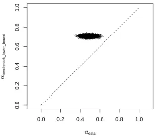
The result is shown in Figure 3: forall104posterior draws, α∗(benchmark model)> αdata
which means that the result is extremely unlikely to be an artifact of the sample size.
0.0 0.2 0.4 0.6 0.8 1.0
0.00.20.40.60.81.0
αdata
αbenchmark_lower_bound
Figure 3: Posteriorαdatavs the lower boundα∗of the benchmark model, with hypothetical sample size N = 10000,105posterior draws. The45° line is dashed.
4 Extensions
Considering thatα∗> αdatafor all the datasets reviewed in Section 3, we conclude that not only does the benchmark model discussed in Section 2 have a limited range of labor market flows it can generate, but the data appears to lie outside this range and thus the problem is empirically relevant.
In this section we discuss various extensions and check if they alleviate this problem. First, in Section 4.1 we introduce a continuous search effort margin, while in Section 4.2 we explore how state- dependent separation rates affect labor market flows and whether this alleviates the problem—as we
11This increases posterior uncertainty relative to the data: we do this to demonstrate that the results would be robust in an even smaller sample.
shall see, neither of these lowerα∗. In Sections 4.3 and 4.4, we relax the assumption of having the same process for the individual-specific statexfor all workers: since this plays a key role in the derivation of Lemma 1, it is not surprising that both extensions can makeα∗ < αdata. We aim for global analytical results in all of these discussions.
Finally, in Section 4.5 we consider the problem of measurement error in the form of survey mis- classification: first, we provide a general theoretical characterization, then specifically examine the possibility of misclassification between inactivity and unemployment. We find that this is also helpful in matching the model to the data.
4.1 Continuous search effort
The binary search technology in the benchmark model is tractable, but very stylized. Time use studies such as Krueger and Mueller (2012) and Aguiar, Hurst, and Karabarbounis (2013) show that time de- voted to searching for a job displays significant variation across countries, gender, and age, and thus it can be argued that a model with continuous search effort would be more realistic. This section extends the benchmark model with a search effort margin, and shows that when it comes to observed flows, the extended model can be mapped to the benchmark model and thus has the same constraints when it comes to matching observed transition rates between E, U, and I.12
The only change we make to the benchmark model is allowing the non-employed worker to choose the rateφat which offers arrive continuously, by paying a search costc(φ). As is standard, we assume thatcis continuous, nonnegative, strictly increasing, and convex.13The HJB equations are
rN(x) =b(x) + max
φ≥0
get offers at rateφ, pay search costc(φ)
{ φ(
W(x)−N(x))+
−c(φ) }
+γ
state change
( Ex′[
N(x′)]
−N(x) )
(30) rW(x) =w(x) +σ(N(x)−W(x))
exogenous separation
+γ(Ex′[N(x′)∨W(x′)]−W(x))
state change, possibly endogenous separation
(31)
As before, letS(x) =W(x)−N(x)ands(x) =w(x)−b(x)denote the surplus value and the flow surplus. Then we can rewrite (30) and (31) as
(r+σ)S(x) =s(x)−max
φ≥0
{
φS(x)+−c(φ) }
+γ (
Ex′[
S(x′)+]
−S(x) )
The second term on the right hand side is the opportunity cost of not searching, and the third term is the change of value from drawing a newx′. Introduce
φ(x) = argmaxˆ
φ≥0
φS(x)+−c(φ)
to denote the optimal search effort. From the assumptions onc, we know that
φ(x) = 0ˆ whenS(x)≤ 0, and
φˆis increasing inx. Assume that above some search effortφ > 0, non-employed workers are
12
I thank Fabien Postel-Vinay for suggesting this extension.
13
See, for example, Christensen et al. (2005).
classified asunemployed, whereas for
φ(x)ˆ < φworkers are classified asinactive. Let L ={x:S(x)<0}
M ={x: 0≤S(x),φ(x)ˆ < φ}
H ={x:φ≤φ(x)}ˆ
Then define the observed job finding rates for workers inMandHas φm≡
∫
x∈Mφ(x)dFˆ (x) (32)
φh≡
∫
x∈Hφ(x)dFˆ (x) (33)
Since all other parts of the benchmark model are unchanged, it is easy to see that with (32) and (33), observationally this model can be mapped to the benchmark model. Consequently, all the conclusion about the benchmark model apply, in particular, the lower boundα∗is the same as in the benchmark model, and thus this extension does not resolve the discrepancy between the model and the data.
4.2 State-dependent separation rates
In this section, we relax the assumption that exogenous separation rates are the same for all employed workers. We can rationalize this as a reduced-form version of a model in which some jobs are less stable than others: it would not be unreasonable to assume that jobs in which the workers’s surplus is lower are less able to withstand certain kinds of exogenous shocks.14
For analytical simplicity we only distinguish separation rates for marginal and non-marginal work- ers: non-marginal workers separate at rateσ, while marginal workers separate at a higher rateσ+δσ, whereδσ ≥0. Everything else is the same as in the benchmark model: in particular, the only observed flow that is different compared to the benchmark model is
λEI=µ(σ+δσ) +qℓ (34)
Consequently,
λE⌊IU⌋=σ+µδσ+qℓ (35)
The flow balance equations (11)–(14) are unchanged, but foremandehwe have em·(qℓ+qh+δσ+σ) =eh·qm+ (mm−em)·φm
eh·(qm+qℓ+σ) =em·qh+ (mh−eh)·φh
Similarly to Section 2, we first derive simpler bounds forα: leaving inqℓandδσas free parameters and
14I thank Christian Haefke for suggesting this extension.