Forecasting the Effects of In-Store Marketing on Conversion Rates for Online Shops
Holger Fink
1,2,* and Yvonne Graf
31
Department of Computer Science and Mathematics, Munich University of Applied Sciences, Lothstrasse 64, 80335 Munich, Germany
2
Center for Quantitative Risk Analysis, Department of Statistics, Ludwig-Maximilians-Universität München, Akademiestrasse 1/I, 80799 Munich, Germany
3
Chair of Strategic Industrial Marketing, Institute of Business Administration, University of Regensburg, Universitätsstrasse 31, 93053 Regensburg, Germany; yvonne.graf@wiwi.uni-regensburg.de
* Correspondence: holger.fink@hm.edu; Tel.: +49-89-1265-3707
Received: 14 July 2018; Accepted: 10 September 2018; Published: 13 September 2018
Abstract: As webstores usually face the issue of low conversion rates, finding ways to effectively increase them is of special interest to researchers and practitioners alike. However, to the best of our knowledge, no one has yet empirically investigated the usefulness of various in-webstore marketing tools like coupons or different types of product recommendations. By analysing clickstream data for a shoe and a bed online store, we are contributing to closing this gap. In particular, we use our present data to build more general hypotheses on how such purchasing incentives might function and on how they could be used in practice.
Keywords: online shop; purchase incentive; conversion rate; coupon; clickstream
1. Introduction
Throughout the last several years, internet advertising revenue has grown constantly to about
$59.6bn in the U.S. alone (see Figure 1) with the pace notably picking up since 2010. Parallel to this development, according to a recent release from the U.S. Department of Commerce, the retail e-commerce sales share of total retail sales has nearly doubled from about 4% in 2010 to 8.1% in 2016 (cf. [1]).
2001 2002 2003 2004 2005 2006 2007 2008 2009 2010 2011 2012 2013 2014 2015
US Internet Advertising Revenue
0bn 10bn 20bn 30bn 40bn 50bn 60bn 70bn
Figure 1. US Internet Advertising Revenue from 2001 to 2015. Source: [1].
Forecasting2019,1, 70–89; doi:10.3390/forecast1010006 www.mdpi.com/journal/forecasting
As such trends are usually accompanied by increasing competition, two main challenges arise for online retailers which we will discuss in more detail below. Due to the general direction of the present paper, we shall especially focus on the second one. For a more general overview of marketing in computer-mediated environments (which is beyond the scope of our paper), we refer to [2].
Firstly, customers need to find their way to a shop’s website which can be facilitated by, e.g., search engine optimization (SEO), contextual search engine advertising (SEA) or graphical banner advertising (see, e.g., [3–5] or the very recent studies of [6,7]).
Secondly, once potential customers have reached a webstore, they need to be “encouraged” to actually convert from visitor to buyer. In the literature, there can be found various discussions on how to increase this conversion rate. For once, especially in the earlier days of e-commerce, trust played an important role and could be increased by investing in the general design of an online shop to project the ability of a certain quality in terms of products and services (cf. [8–13]). However, the detailed shape, style and content of a website or a shop can also boost the conversion rate if it fits to the characteristics of the targeted customer group (cf. [14]). This can go as far as having a webstore that automatically
“morphs” to match the suspected needs of each specific visitor (cf. [15]). In this context, based on their generated clickstream data (i.e., how they move through a webpage), customers can be characterized either by statistical methods or, more dynamically, by certain learning models (cf. [16]) in order to specifically target them with in-store marketing.
However, due to the rare academic availability of such clickstream data containing in-webstore marketing campaigns, the relevant literature here is still scarce. However, by partnering up with a digital consulting start-up that specializes in increasing the effectiveness of webshops by boosting their conversion rates, we were able to obtain such a unique data set from two stores in the online retail space—a shoe and a bed shop. This provides us with the possibility to investigate two very different product types as shoes and beds differ significantly in various characteristics (price, duration of use, etc.).
Therefore, in the present paper, we are aiming to further close the above-mentioned research gap by examining the impact of different types of (in-store) purchasing incentives on each shop’s conversion rate. Additionally, we cast a further glance on the forecasting power of general clickstream data extending earlier in-store studies (cf. [17–21]). In more detail, we measure the conversion rate effects of advertising in the form of coupons, product sliders (i.e., “Other products that might interest you:”) or information about the shopping behaviour of peers (i.e., “Other customers bought these products:”). Additionally, we account for individual-specific exogenous effects captured by clickstream data like how the customer reached the online shop or how many pages he viewed.
Our work adds to current research in two ways: to the best of our knowledge, this is the first time that the effects of in-webstore marketing approaches like coupons have been empirically measured via clickstream data. Additionally, we suggest certain data-driven hypotheses built from our data on how such purchasing incentives could be used best in practice.
The structure of our article is as follows: after a thorough literature review carried out in the next section (“Relevant Literature”), we discuss the present data set and investigate the potential effects of purchasing incentives from a more descriptive standpoint in “Data”. To address any bias in statistical tests due to potentially non-random selection of control and target groups in our data, we invoke classical generalized models of the logit-type (“Statistical Model Setup”). We present our results in
“Empirical Findings” and extensively discuss the impact of certain purchasing incentives allowing possible interactions with other exogenous variables. Finally, in “Conclusions and Implications”, we summarize our approach and give recommendations on how to generally identify customer groups which can be purposely targeted to boost an online shop’s conversion rate.
All statistical analyses in the present paper have been carried out with the software
package R-3.5.1.
Relevant Literature
A first step towards selling products and services online is obviously taken by attracting users to a webshop which can, e.g., either be done via SEO, contextual SEA (cf., e.g., [22–24]) or (graphical) banner ads. With the availability of various types of clickstream data, i.e., information about how users move through the web, a large part of online advertising research has focussed on such contextual and graphical ads, although it might be difficult to deduce direct effects: in this context, Xu et al. [25] find that banner ads have a rather low impact on direct conversion rates but might encourage future site visits via different advertising formats. Their study is, however, limited in the sense that their data does not contain visits resulting from non-paid search engine results or direct URL type-ins.
An important insight was that, due to some kind of information overflow, the use of display ads is accompanied by the risk of avoidance (cf. [3]). In order to counteract this effect, such ads can be customized or personalized to catch the attention of users (cf. [4,6,7,26–28] or the recent study of [14]).
In addition, one can increase the obtrusiveness of ads which has been shown to positively impact visitors’ purchase intentions even though a combination of both approaches might be harmful due to privacy concerns (cf. [5,28,29]).
In general, behavioural targeting, personalized advertising or so-called website morphing (cf. [15]) has become a deeply investigated research stream.
However, all of these studies focus somewhat on increasing conversion rates by attracting users to a webstore. Therefore, in a second step, one might also ask how in-webstore advertising might be helpful to convert users which have already found their way to a shop by, e.g., offering time-limited price discounts or luring visitors to view certain products in more detail. The effect of such coupons and general in-store marketing campaigns has already been extensively studied in real-world offline stores over the last decades:
As it is well-known, one advantage of coupons lies in their simplicity as a marketing tool (cf. [30]). At first, to asses their effectiveness, several authors considered just the pure redemption rate, i.e., the number of coupons which are being used compared to the amount which has been distributed (see [31]). In addition, Reibstein and Traver [31] developed a model to determine various factors which influence the redemption rate, namely (amongst other things) the method of distribution, the face value of coupons and the discount offered by the coupon.
However, later on, Bawa and Shoemaker [32] pointed out that redemption rates as a single measure of success are misleading as high rates are not equal to profitability (cf. [33]). They suggested to rather focus on incremental sales and tried to identify target households which are most lucrative.
Dhar and Hoch [34] concluded that the effect of in-store coupons for grocery chains might be larger than the one for off-the-shelf price discounts while [35] pointed out that the mere exposure to customized coupons might have a positive effect on sales and profitability while such coupons work better when they are unexpected.
In a more recent study, Reichhart et al. [36] compared digital e-mail and mobile text message coupons by conducting a field experiment with exposed users from an opt-in database. They could find that text message delivery caused better conversion rates even though the response rates proofed to be lower. In a similar context, Danaher et al. [37] conducted a two-year trial in a shopping mall with similar text message coupons and found that traditional offline coupon characteristics, e.g., face value, are again the main influencing factor for coupon effectiveness. In addition, the authors found that location and time of delivery influence redemption, e.g., customers tend to redeem a coupon more often if the corresponding store is closer. Additionally, they suggest that a shorter expiration length has a positive effect as they signal urgency to customers.
Next to coupons, more general in-store marketing campaigns are in the focus of current research,
as well. For example, Chandon et al. [38] conducted an eye-tracking experiment and concluded that,
even though the number of product facings has a positive effect on conversion rate for certain types
of shop visitors, gaining attention is itself not always sufficient to increase sales. Inman et al. [39]
carried out several intercept interviews and identified characteristics of shop visitors that tend to make unplanned purchases.
More recently, Hui et al. [40,41] investigated visitors of a grocery store by video-tracking and identified product categories that are more likely to elicit unplanned purchases than others.
Additionally, they suggest that coupons which tempt customers to deviate from their determined in-store travel path are nearly twice as effective as those who do not. Furthermore, Zhang et al. [42]
concluded that interactive social influences can positively affect sales as well, especially when shoppers show certain behavioral cues.
Having all the above mentioned in-store marketing research available, it might be an obvious step to straightforwardly transfer these results to webstores. However, as Bucklin et al. [43] pointed out, there are major differences between the choice making processes of online customers and classical real-life shop visitors that can influence the impact of customized promotions (see, e.g., [44]). As a consequence, it is not clear if obtained results on coupons and in-store marketing do hold in a digital world. In fact, the relevant literature does not yet provide a final answer.
As the conversion rate of a typical online shop rarely exceeds 5% (cf. [17]), a large part of early studies focussed on identifying visitors who are more likely to buy than others. In this context, based on clickstream data for an online-shop selling cars, Sismeiro and Bucklin [19] decomposed the purchasing process into several steps describing each one with a probit model. In particular, they find that repeated visits do per se not go hand in hand with a higher conversion rate—even though an earlier study suggested that browsing behaviour might change in such situations (see [45]).
In more detail, Moe and Fader [17,18] found evidence that even though customers who visit an retail online-store more frequently tend to have a higher conversion rate, this is mainly due to the subgroup of shoppers whose frequency behaviour actually increased over time.
In terms of directly increasing conversion rates, Wilson [46] suggested potential positive impacts of easier and more transparent purchase/checkout processes as well as free-shipping promotions in a B2B context even though their study is only based on several hundred shop visitors.
More generally speaking, an understanding of customer decision rules in online stores (cf. [20]) could be used for individual promotional targeting. In this context, Schellong et al. [21] (extending an earlier study of [47]) try to classify the in-store shopping behaviour of a fashion retailer’s visitors by clustering browsing and search patterns.
Still, while several of the above studies already suggested that targeted in-store marketing based on clickstream data might be a fruitful approach, detailed empirical evidence on various such techniques has been scare. One of the few exceptions is the study of [48] who investigate the effect of showing visitors personalized product recommendations. In the following, by partnering up with a digital consulting start-up, we aim to further close this research gap by studying the effects of various in-store marketing campaigns, especially the impact of time-limited discounts in the form of coupons and certain types of product recommendations.
2. Data
In this section, we want to briefly describe our data set and provide a first descriptive overview.
In particular, we received a month of customer data from two different mid-sized online shops from
our research partner, a start-up in the e-commerce space. These shops shall henceforth be denoted by
their specific business sector, i.e., “shoe shop” and “bed shop”. The chosen month is February 2015 for
which we have data from 1 February 2015 to 28 February 2015 for the shoe and from 6 February to
15 February for the bed shop. The reasoning behind this time period is that no particularly large public
holiday (which might bias our results) falls within this month. Additionally, the data is outdated
enough such that one should not be able to draw any conclusion on the identity of the individual
shops. This is especially important from a compliance perspective as, due to our agreement with
our research partner, we are not allowed to share precise information about the specific online stores.
In particular, we were not provided with details about the stores’ websites (like their design, style of product presentation, etc.).
Similarly to, e.g., the study of [7], our data is available on a cookie level which can have several drawbacks in terms of user identifiability (cf. [7,49] for a more detailed discussion) but is still industry standard.
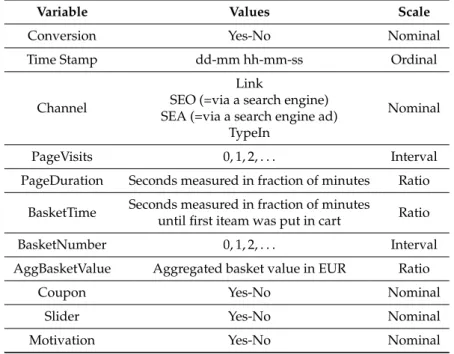
For each user/cookie, we have information about the particular day and time of his visit, how he reached the website and for how long he stayed, how many pages he viewed, if and when he put any items in the shopping cart, the aggregated value in EUR of these, if he actually converted and whether he was shown any purchasing incentives like a ’Coupon’ (cash value between 5–10 EUR), a ’Slider’
(“Other products that might interest you:”) or a ’(Group) Motivation’ ad (“Other customers bought these products:”). Table 1 summarizes these available variables and their scales.
Table 1. Available variables, potential values and scales in our clickstream data set.
Variable Values Scale
Conversion Yes-No Nominal
Time Stamp dd-mm hh-mm-ss Ordinal
Channel
Link
Nominal SEO (=via a search engine)
SEA (=via a search engine ad) TypeIn
PageVisits 0, 1, 2, . . . Interval
PageDuration Seconds measured in fraction of minutes Ratio BasketTime Seconds measured in fraction of minutes
Ratio until first iteam was put in cart
BasketNumber 0, 1, 2, . . . Interval
AggBasketValue Aggregated basket value in EUR Ratio
Coupon Yes-No Nominal
Slider Yes-No Nominal
Motivation Yes-No Nominal
After removing incomplete data points and transmission errors, we are left with a total of 266,773 visits for the shoe and 98,266 for the bed shop. Of these numbers, a total of 188,430 (70.63%) and 76,728 (78.08%) visitors are unique from a cookie level standpoint, i.e., the rest arises due to various users visiting the stores on multiple occasions during February 2015. From a statistical point of view, as a consequence, our individual data points are probably not perfectly independent but might (depending on the user behaviour) correlate. Given the comparably small amount of data available for our study, it is hard to adequately account for such dependence effects: to visualize this issue, let us assume that the impression of an initial shop visit stays with the average user for about seven days.
Then, even when we fully accounted for multiple visits, about 25% of our data might be diluted by such effects without us even knowing. Therefore, for the sake of simplicity, we shall from now on model each cookie as being a unique visitor. However, we want to stress that this is probably the biggest drawback of our study and needs to be addressed in future research.
As a consequence of the above and in line with comparable studies (e.g., [7]), we will not aim to
generalize the results of our study to different shops and time periods but rather use our present data
for a more exploratory approach trying to understand how purchase incentives might affect users and
build data-driven hypotheses for a more general framework.
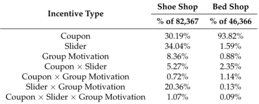
Table 2 provides a global summary of our data situation and shows that about 30% of all visits for the shoe and about 50% for the bed shop were shown some purchasing incentives. Regarding the nature of such influences, Table 3 shows that around 73% for the first and 96% for the second shop were of a unique type while the rest is mostly a combination of two. Given the small amount of observations for multiple incentives, we shall neglect any potential interactions effects between these for the analysis to come.
Table 2. Number of observations with and without having seen some purchasing incentives.
Type Observations Overall Observations without Incentive Observations with Incentive Absolute Absolute % of Overall Absolute % of Overall
Shoe Shop 266,773 184,406 69.12% 82,367 30.88%
Bed Shop 98,266 51,900 52.82% 46,366 47.18%
Table 3. Distribution of unique purchasing incentives and their combinations for both shops.
Incentive Type Shoe Shop Bed Shop
% of 82,367 % of 46,366
Coupon 30.19% 93.82%
Slider 34.04% 1.59%
Group Motivation 8.36% 0.88%
Coupon × Slider 5.27% 2.35%
Coupon × Group Motivation 0.72% 1.14%
Slider × Group Motivation 20.36% 0.13%
Coupon × Slider × Group Motivation 1.07% 0.09%
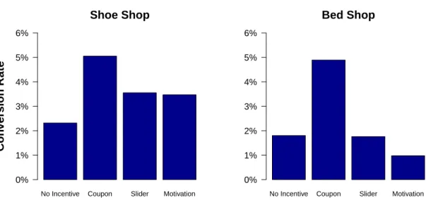
Considering the sales of the individual shops and splitting all users into a non-influenced and an incentivised group, we can clearly see that the conversion rate roughly doubles for both stores once at least one purchasing incentive has been shown. A simple two-sided binomial test confirms that these results are significant on all sensible levels, see Table 4, even though the actual effects differ substantially as can be seen by Figure 2.
Table 4. Conversion rates and simple binomial tests regarding the effectiveness of purchasing incentives.
Type Conversion Rate Two-Sided Binomial Test
Overall No Incentive With Incentive Test Statistic
p-ValueShoe Shop 3.02% 2.32% 4.59% − 31.71 0.000
Bed Shop 3.24% 1.80% 4.85% − 26.93 0.000
No Incentive Coupon Slider Motivation
Shoe Shop
Con ver sion Rate
0%
1%
2%
3%
4%
5%
6%
No Incentive Coupon Slider Motivation
Bed Shop
0%
1%
2%
3%
4%
5%
6%
Figure 2. Conversion rates for non-influenced visitors and those who have been shown a unique purchasing incentive.
However, it is hard to draw robust conclusions based on these tests as one needs to ensure that both groups, non-influenced and incentivised visitors, consist of users having the same overall characteristics. Otherwise, it would be quite easy to manipulate the effects of purchasing incentives by showing these mostly to such visitor groups which already have an ex-ante higher conversion rate.
Even though our research partner ensured us that the selection of incentivised customers was “mostly random”, we want to address this issue in more detail.
As a first step, for both shops, we split all users into non-influenced and incentivised groups.
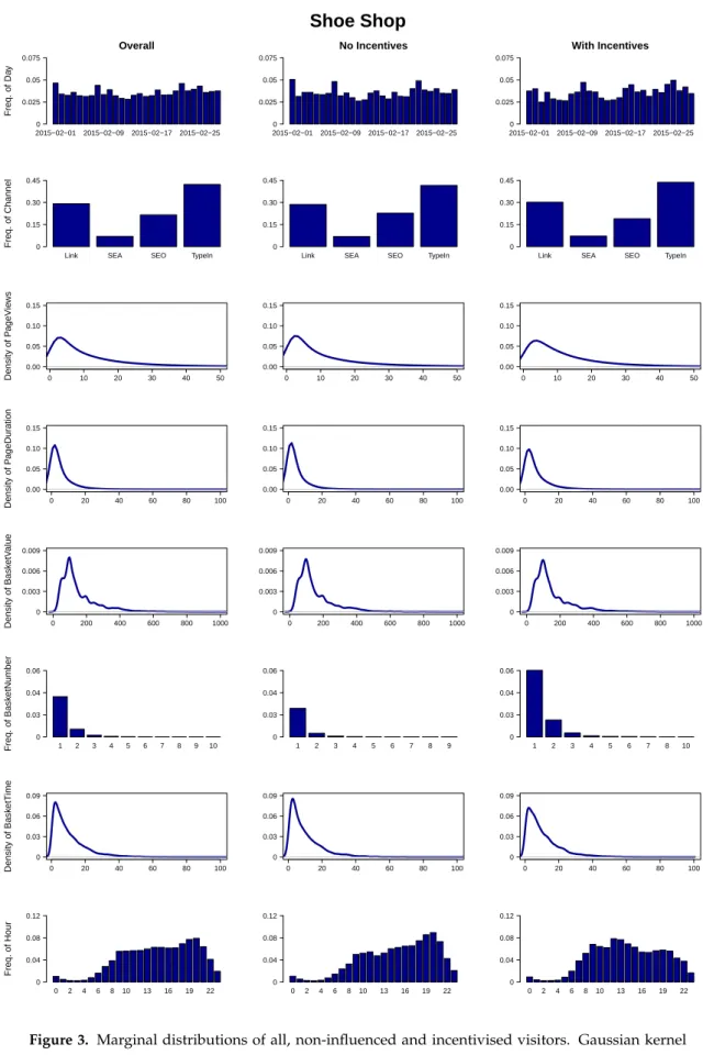
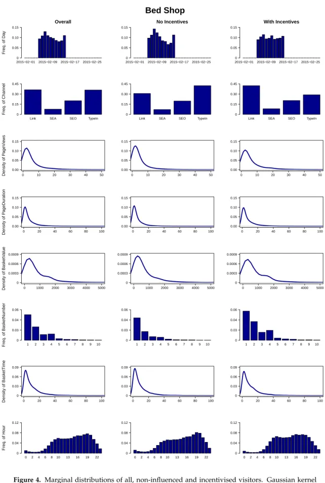
Now, Figures 3 and 4 present the marginal distributions of all collected variables for each store in total and broken down into the “control” and “test” customer categories. Even though these plots look mostly fine, a few differences spring into view: for example, for the shoe shop the frequencies of at least one item in the shopping basket are higher for influenced users. However, this makes sense as purchasing incentives are usually not directly shown from the start but only after the visitor stays some time on the shop’s webpage. As a larger group of customers leaves our online stores directly after a few seconds, the difference in the frequencies can (partly) be explained. However, more worrisome is, e.g., the mismatch for the bed shop and the variable ‘Channel’. Apparently, the share of visitors which typed the shops address directly into the browser is underrepresented in the incentivised group.
From our perspective, this is a clear violation of having a completely random allocation of incentives.
Therefore, we do not feel comfortable relying on the results of binomial tests as carried out in Table 4.
However, as we will discuss in the next section, our chosen statistical approach of applying generalized
linear models allows us to tackle and mitigate such “non-randomness”. Additionally, we will provide
a minimal working example to show that these setups can efficiently detect if a conversion rate increase
for incentivised users is only due to a unclean or tactical selection of the target group or due to the
purchasing incentive itself.
2015−02−01 2015−02−09 2015−02−17 2015−02−25
Overall
Freq. of Day
0 0.025 0.05 0.075
Link SEA SEO TypeIn
Freq. of Channel 0 0.15 0.30 0.45
0 10 20 30 40 50
Density of PageViews
0.00 0.05 0.10 0.15
0 20 40 60 80 100
Density of PageDuration
0.00 0.05 0.10 0.15
0 200 400 600 800 1000
Density of BasketValue
0 0.003 0.006 0.009
1 2 3 4 5 6 7 8 9 10
Freq. of BasketNumber
0 0.03 0.04 0.06
0 20 40 60 80 100
Density of BasketTime
0 0.03 0.06 0.09
0 2 4 6 8 10 13 16 19 22
Freq. of Hour
0 0.04 0.08 0.12
2015−02−01 2015−02−09 2015−02−17 2015−02−25
No Incentives
0 0.025 0.05 0.075
Link SEA SEO TypeIn
0 0.15 0.30 0.45
0 10 20 30 40 50
0.00 0.05 0.10 0.15
0 20 40 60 80 100
0.00 0.05 0.10 0.15
0 200 400 600 800 1000
0 0.003 0.006 0.009
1 2 3 4 5 6 7 8 9
0 0.03 0.04 0.06
0 20 40 60 80 100
0 0.03 0.06 0.09
0 2 4 6 8 10 13 16 19 22
0 0.04 0.08 0.12
2015−02−01 2015−02−09 2015−02−17 2015−02−25
With Incentives
0 0.025 0.05 0.075
Link SEA SEO TypeIn
0 0.15 0.30 0.45
0 10 20 30 40 50
0.00 0.05 0.10 0.15
0 20 40 60 80 100
0.00 0.05 0.10 0.15
0 200 400 600 800 1000
0 0.003 0.006 0.009
1 2 3 4 5 6 7 8 10
0 0.03 0.04 0.06
0 20 40 60 80 100
0 0.03 0.06 0.09
0 2 4 6 8 10 13 16 19 22
0 0.04 0.08 0.12
Shoe Shop
Figure 3. Marginal distributions of all, non-influenced and incentivised visitors. Gaussian kernel
density estimators have been used for continues variables. ’BasketNumber’ frequencies are only shown
for one and more items for better visibility.
2015−02−01 2015−02−09 2015−02−17 2015−02−25
Overall
Freq. of Day
0 0.05 0.10 0.15
Link SEA SEO TypeIn
Freq. of Channel 0 0.15 0.30 0.45
0 10 20 30 40 50
Density of PageViews
0.00 0.05 0.10 0.15
0 20 40 60 80 100
Density of PageDuration
0.00 0.05 0.10 0.15
0 1000 2000 3000 4000 5000
Density of BasketValue
0 0.0003 0.0006 0.0009
1 2 3 4 5 6 7 8 9 10
Freq. of BasketNumber
0 0.03 0.04 0.06
0 20 40 60 80 100
Density of BasketTime
0 0.03 0.06 0.09
0 2 4 6 8 10 13 16 19 22
Freq. of Hour
0 0.04 0.08 0.12
2015−02−01 2015−02−09 2015−02−17 2015−02−25
No Incentives
0 0.05 0.10 0.15
Link SEA SEO TypeIn
0 0.15 0.30 0.45
0 10 20 30 40 50
0.00 0.05 0.10 0.15
0 20 40 60 80 100
0.00 0.05 0.10 0.15
0 1000 2000 3000 4000 5000
0 0.0003 0.0006 0.0009
1 2 3 4 5 6 7 8 9 10
0 0.03 0.04 0.06
0 20 40 60 80 100
0 0.03 0.06 0.09
0 2 4 6 8 10 13 16 19 22
0 0.04 0.08 0.12
2015−02−01 2015−02−09 2015−02−17 2015−02−25
With Incentives
0 0.05 0.10 0.15
Link SEA SEO TypeIn
0 0.15 0.30 0.45
0 10 20 30 40 50
0.00 0.05 0.10 0.15
0 20 40 60 80 100
0.00 0.05 0.10 0.15
0 1000 2000 3000 4000 5000
0 0.0003 0.0006 0.0009
1 2 3 4 5 6 7 8 9 10
0 0.03 0.04 0.06
0 20 40 60 80 100
0 0.03 0.06 0.09
0 2 4 6 8 10 13 16 19 22
0 0.04 0.08 0.12
Bed Shop
Figure 4. Marginal distributions of all, non-influenced and incentivised visitors. Gaussian kernel
density estimators have been used for continues variables. ’BasketNumber’ frequencies are only shown
for one and more items for better visibility.
3. Statistical Model Setup
This section shall provide an overview of our chosen statistical approach. As we are aiming to econometrically model the impact of several exogenous (mostly categorical) variables on each shop’s endogenous conversion rate, we chose a classical logistic regression setup, i.e., a generalized linear model with logit link. In the following, we shall briefly review the necessary properties of such setups.
For a more detailed background, we refer an interested reader to, e.g., [50].
Now, in particular, for the ith visitor, the (conditional) probability of a purchase is assumed to be determined via
π
i= P ({ ith visitor converts }| X
i, β ) = exp ( X
iβ )
1 + exp ( X
iβ ) , (1)
where X
i= ( 1, X
i1, X
i2, . . . , X
mi) contains the realizations of the exogenous m variables (and 1 to include an intercept) for the ith visitor and β = ( β
0, β
1, β
2, . . . , β
m) represents the model parameters.
Given the data of n visitors, an estimator β ˆ for the logit model’s parameters can be obtained via maximum likelihood (ML). For any specific visitor characterized by X
i, the model-implied conversion probability forecast is calculated via
ˆ
π
i= exp ( X
iβ ˆ )
1 + exp ( X
iβ ˆ ) . (2)
In particular, we shall consider three different model setups:
Model 1 (Reference/“Raw Benchmark Model”):
Xiβ = β0 + β1Month (1–10) + β2Month (20–28)
+ β3Weekend + β4Channel(Link) + β5Channel(SEA) + β6Channel(SEO) + β7PageViews + β8PageDuration + β9AggBasketValue + β10BasketNumber + β11Hour (0–7) + β12Hour (8–12) + β13Hour (19–23)
Model 2 (with Incentives):
Xiβ = β0 + β1Month (1–10) + β2Month (20–28)
+ β3Weekend + β4Channel(Link) + β5Channel(SEA) + β6Channel(SEO) + β7PageViews + β8PageDuration + β9AggBasketValue + β10BasketNumber + β11Hour (0–7) + β12Hour (8–12) + β13Hour (19–23)
+ β14Coupon + β15Slider + β16Motivation
Model 3 (with Incentives & Interactions):
Xiβ = β0 + β1Month (1–10) + β2Month (20–28)
+ β3Weekend + β4Channel(Link) + β5Channel(SEA) + β6Channel(SEO) + β7PageViews + β8PageDuration + β9AggBasketValue + β10BasketNumber + β11Hour (0–7) + β12Hour (8–12) + β13Hour (19–23)
+ β14Coupon + β15Slider + β16Motivation
+ β17Coupon×Month (1–10) + . . . + β30Coupon×Hour (19–23) + β31Slider×Month (1–10) + . . . + β34Slider×Hour (19–23) + β35Motivation×Month (1–10) + . . . + β38Motivation×Hour (19–23).
(3)
In particular, we chose ‘TypeIn’ as a reference category for ‘Channel’, ‘13–18’ (abbreviating
‘13:00:00–18:59:59’) for ‘Hour’ and ‘11–19’ for ‘Month’.
After obtaining the ML estimates, we can assess each model’s fit by its deviance given by Deviance = − 2
∑
n i=1C
ilog ( π ˆ
i) + ( 1 − C
i) log ( 1 − π ˆ
i) (4)
with
C
i: =
( 1, ith visitor converts,
0, else, (5)
which basically measures the difference between the likelihood of the chosen setup and a fully saturated model. Therefore, the smaller the deviance, the better the in-sample fit of the present model.
The deviance of a model with just a constant is called null deviance. Additionally, having two nested setups, the difference between both deviances is χ
2-distributed under the null hypothesis of the smaller model being the correct one. To further asses the validity of our models, we shall make use of the Akaike information criterion (AIC) as well.
In a first step, we want to test whether the larger models have an advantage over the smallest one implying that at least one influence-type has a significant impact on the conversion rate. Additionally, as from a practical perspective, a shop’s owner would be interested in identifying certain visitors for which incentives are most effective, we shall furthermore consider the significance of each individual incentive including potential interaction effects. Regression coefficients thus can be interpreted via their implied ceteris paribus changes on the conversion odds. Generally, when it comes to interaction effects, additional care has to be taken (cf. [51]). However, as Model 3 only includes interactions between a dummy and one other variable, we are on the safe side here.
Finally, we can investigate each setup’s in-sample forecasting capabilities by assuming that ˆ
π
i> 0.5 implies a predicted conversion for the ith visitor. Considering a 2 × 2-cross table, we can check how much the forecasts agree with the actual data. Similarly, we shall check the out-of-sample prediction power by randomly separating our data into a training and a test set. Then, in a first step, the parameters β are estimated on the training data and the actual model forecasts are then evaluated for the test set.
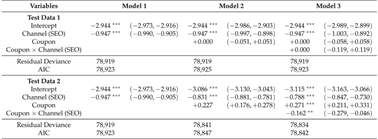
As indicated in the previous section, it remains to illustrate how our chosen logistic regression approach mitigates and tackles the issue of potential “non-randomness” in our data. For this purpose, let us generate a test data set (called ’Test Data 1’) with 300,000 observations and (only) two exogenous variables present: Channel (TypeIn or SEO) and Coupon (Yes or No) (see Table 5). Additionally, we assume that the coupons have no influence while SEO-visitors convert in 2.0% and TypeIn-visitors in 5.0% of all cases. Now, if we show a coupon to 10% of all SEO- and 60% of the TypeIn-visitors (distributed such that the independence assumption between coupon and sale holds) a simple binomial test would indicate a significant conversion rate difference between influenced and non-influenced customer groups, see Table 6. However, invoking all three introduced types of logistic regression setups (see Table 7), it becomes clear that this seemingly significant effect is just an artificial one due to the obviously inappropriate distribution of the coupon variable.
Table 5. Artificially generated test data.
Data Channel (SEO) Channel (TypeIn) Test Data 1 No Sale Sale No Sale Sale No Coupon 176,400 3600 38,000 2000
Coupon 19,600 400 57,000 3000
Test Data 2 No Sale Sale No Sale Sale No Coupon 176,440 3560 38,300 1700
Coupon 19,560 440 56,700 3300
Table 6. Conversion rates and simple binomial tests regarding the effectiveness of purchasing incentives
Data Type Conversion Rate Binomial Test
Overall No Incentive With Incentive Test Statistic
p-ValueTest Data 1 3.00% 2.55% 4.25% − 24.20 0.000
Test Data 2 3.00% 2.39% 4.68% − 32.43 0.000
Similarly, we generate a second data set (’Test Data 2’) equal to the first one. However, the effect of coupons within the channel-groups is made such that, for SEO-clients, the conversion rate is approximately 11.2% higher through the purchase incentive while, for TypeIn-visitors, the effect is even 29.4%. A simple binomial test as carried out in Table 6 can not differentiate both data sets while our logistic regressions neatly catches even the interaction effect between both exogenous variables as illustrated by Table 7: Model 2 implies that on average a coupon increases the purchasing odds by exp (+ 0.227 ) − 1 = 25.5% while Model 3 indicates exp (+ 0.271 ) − 1 = 31.1% higher odds for TypeIn-visitors and an exp (+ 0.271 − 0.162 ) − 1 = 11.5% increase for SEO-customers.
Table 7. Logistic regression models for our test data. Null deviance equals 80,845 for both data sets.
p-values equal or below 0.05/0.01/0.001 are indicated by
∗/
∗∗/
∗∗∗.
Variables Model 1 Model 2 Model 3
Test Data 1
Intercept −2.944∗∗∗ (−2.973,−2.916) −2.944∗∗∗ (−2.986,−2.903) −2.944∗∗∗ (−2.989,−2.899) Channel (SEO) −0.947∗∗∗ (−0.990,−0.905) −0.947∗∗∗ (−0.997,−0.898) −0.947∗∗∗ (−1.003,−0.892)
Coupon +0.000 (−0.051,+0.051) +0.000 (−0.058,+0.058)
Coupon×Channel (SEO) +0.000 (−0.119,+0.119)
Residual Deviance 78,919 78,919 78,919
AIC 78,923 78,925 78,923
Test Data 2
Intercept −2.944∗∗∗ (−2.973,−2.916) −3.086∗∗∗ (−3.130,−3.043) −3.115∗∗∗ (−3.163,−3.066) Channel (SEO) −0.947∗∗∗ (−0.990,−0.905) −0.831∗∗∗ (−0.881,−0.781) −0.788∗∗∗ (−0.847,−0.730)
Coupon +0.227 (+0.176,+0.278) +0.271∗∗∗ (+0.211,+0.331)
Coupon×Channel (SEO) −0.162∗∗ (−0.279,−0.046)
Residual Deviance 78,919 78,841 78,834
AIC 78,923 78,847 78,842
4. Empirical Findings
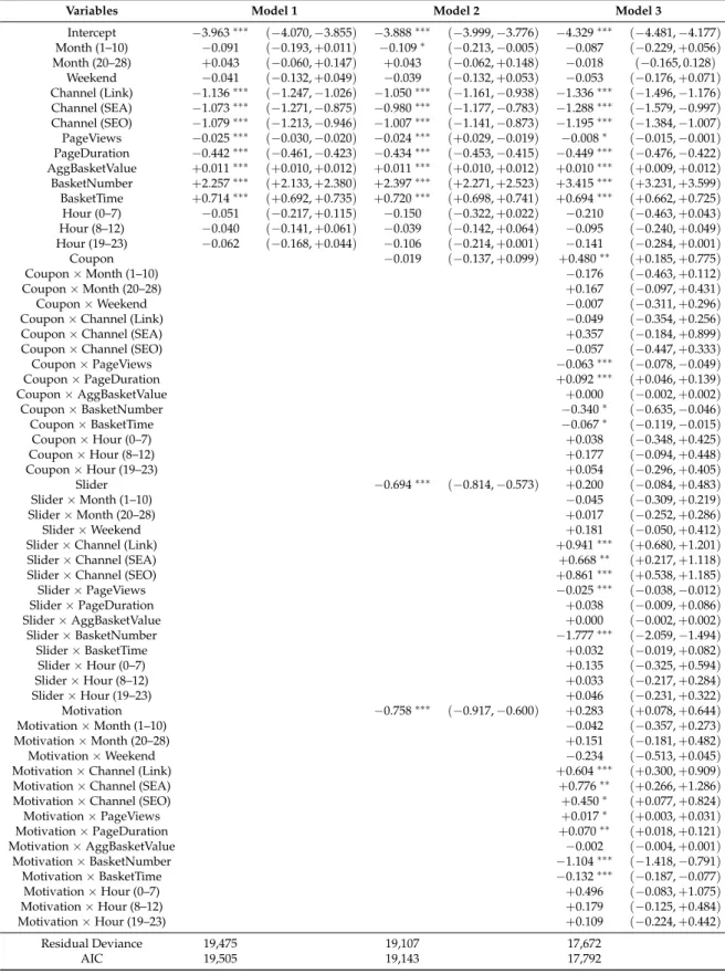
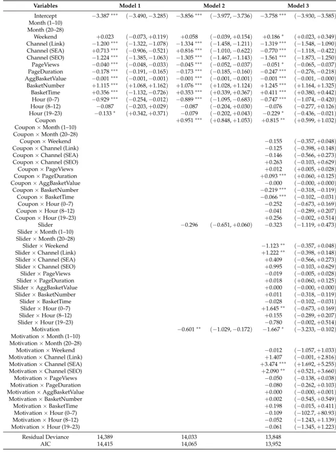
In this section, we shall discuss the obtained results from Model 1–3 for each shop which are individually presented in Tables 8 and 9.
4.1. Results on Shoes
Starting with our shoe shop data and the raw benchmark model, we see that users who actually type the store’s web address manually into their browser are significantly more likely to make a purchase than visitors coming from any other source. In fact, all other things being equal, the conversion odds decrease between 66–68% for all other groups. Furthermore, these odds are reduced by around 2.5% for each additional page view while they decrease by around 36% for any additional minute on the shops website. Obviously, this relationship is truly rather nonlinear and we should not rely too much on the actual numbers even though they confirm the reasonable conjecture that with time, the conversion probability of users goes down. Additionally, as we can see by considering the coefficient of the variable ‘BasketTime’, this decay is countered if visitors actually put some items into their digital shopping cart.
Interestingly, for our shoe shop (and partly in contrast to the bed store), users with more items
in the basket and a higher total basket value are also more likely to buy, which might, however, be
explained by assumingly higher return rates. Sadly, these were not available to confirm our hypothesis.
Table 8. Logistic regression models for our shoe shop data. Null deviance equals 72,216. p-values equal or below 0.05/0.01/0.001 are indicated by
∗/
∗∗/
∗∗∗.
Variables Model 1 Model 2 Model 3
Intercept −3.963∗∗∗ (−4.070,−3.855) −3.888∗∗∗ (−3.999,−3.776) −4.329∗∗∗ (−4.481,−4.177) Month (1–10) −0.091 (−0.193,+0.011) −0.109∗ (−0.213,−0.005) −0.087 (−0.229,+0.056) Month (20–28) +0.043 (−0.060,+0.147) +0.043 (−0.062,+0.148) −0.018 (−0.165, 0.128)
Weekend −0.041 (−0.132,+0.049) −0.039 (−0.132,+0.053) −0.053 (−0.176,+0.071) Channel (Link) −1.136∗∗∗ (−1.247,−1.026) −1.050∗∗∗ (−1.161,−0.938) −1.336∗∗∗ (−1.496,−1.176) Channel (SEA) −1.073∗∗∗ (−1.271,−0.875) −0.980∗∗∗ (−1.177,−0.783) −1.288∗∗∗ (−1.579,−0.997) Channel (SEO) −1.079∗∗∗ (−1.213,−0.946) −1.007∗∗∗ (−1.141,−0.873) −1.195∗∗∗ (−1.384,−1.007) PageViews −0.025∗∗∗ (−0.030,−0.020) −0.024∗∗∗ (+0.029,−0.019) −0.008∗ (−0.015,−0.001) PageDuration −0.442∗∗∗ (−0.461,−0.423) −0.434∗∗∗ (−0.453,−0.415) −0.449∗∗∗ (−0.476,−0.422) AggBasketValue +0.011∗∗∗ (+0.010,+0.012) +0.011∗∗∗ (+0.010,+0.012) +0.010∗∗∗ (+0.009,+0.012) BasketNumber +2.257∗∗∗ (+2.133,+2.380) +2.397∗∗∗ (+2.271,+2.523) +3.415∗∗∗ (+3.231,+3.599) BasketTime +0.714∗∗∗ (+0.692,+0.735) +0.720∗∗∗ (+0.698,+0.741) +0.694∗∗∗ (+0.662,+0.725) Hour (0–7) −0.051 (−0.217,+0.115) −0.150 (−0.322,+0.022) −0.210 (−0.463,+0.043) Hour (8–12) −0.040 (−0.141,+0.061) −0.039 (−0.142,+0.064) −0.095 (−0.240,+0.049) Hour (19–23) −0.062 (−0.168,+0.044) −0.106 (−0.214,+0.001) −0.141 (−0.284,+0.001)
Coupon −0.019 (−0.137,+0.099) +0.480∗∗ (+0.185,+0.775)
Coupon×Month (1–10) −0.176 (−0.463,+0.112)
Coupon×Month (20–28) +0.167 (−0.097,+0.431)
Coupon×Weekend −0.007 (−0.311,+0.296)
Coupon×Channel (Link) −0.049 (−0.354,+0.256)
Coupon×Channel (SEA) +0.357 (−0.184,+0.899)
Coupon×Channel (SEO) −0.057 (−0.447,+0.333)
Coupon×PageViews −0.063∗∗∗ (−0.078,−0.049)
Coupon×PageDuration +0.092∗∗∗ (+0.046,+0.139)
Coupon×AggBasketValue +0.000 (−0.002,+0.002)
Coupon×BasketNumber −0.340∗ (−0.635,−0.046)
Coupon×BasketTime −0.067∗ (−0.119,−0.015)
Coupon×Hour (0–7) +0.038 (−0.348,+0.425)
Coupon×Hour (8–12) +0.177 (−0.094,+0.448)
Coupon×Hour (19–23) +0.054 (−0.296,+0.405)
Slider −0.694∗∗∗ (−0.814,−0.573) +0.200 (−0.084,+0.483)
Slider×Month (1–10) −0.045 (−0.309,+0.219)
Slider×Month (20–28) +0.017 (−0.252,+0.286)
Slider×Weekend +0.181 (−0.050,+0.412)
Slider×Channel (Link) +0.941∗∗∗ (+0.680,+1.201)
Slider×Channel (SEA) +0.668∗∗ (+0.217,+1.118)
Slider×Channel (SEO) +0.861∗∗∗ (+0.538,+1.185)
Slider×PageViews −0.025∗∗∗ (−0.038,−0.012)
Slider×PageDuration +0.038 (−0.009,+0.086)
Slider×AggBasketValue +0.000 (−0.002,+0.002)
Slider×BasketNumber −1.777∗∗∗ (−2.059,−1.494)
Slider×BasketTime +0.032 (−0.019,+0.082)
Slider×Hour (0–7) +0.135 (−0.325,+0.594)
Slider×Hour (8–12) +0.033 (−0.217,+0.284)
Slider×Hour (19–23) +0.046 (−0.231,+0.322)
Motivation −0.758∗∗∗ (−0.917,−0.600) +0.283 (+0.078,+0.644)
Motivation×Month (1–10) −0.042 (−0.357,+0.273)
Motivation×Month (20–28) +0.151 (−0.181,+0.482)
Motivation×Weekend −0.234 (−0.513,+0.045)
Motivation×Channel (Link) +0.604∗∗∗ (+0.300,+0.909)
Motivation×Channel (SEA) +0.776∗∗ (+0.266,+1.286)
Motivation×Channel (SEO) +0.450∗ (+0.077,+0.824)
Motivation×PageViews +0.017∗ (+0.003,+0.031)
Motivation×PageDuration +0.070∗∗ (+0.018,+0.121)
Motivation×AggBasketValue −0.002 (−0.004,+0.001)
Motivation×BasketNumber −1.104∗∗∗ (−1.418,−0.791)
Motivation×BasketTime −0.132∗∗∗ (−0.187,−0.077)
Motivation×Hour (0–7) +0.496 (−0.083,+1.075)
Motivation×Hour (8–12) +0.179 (−0.125,+0.484)
Motivation×Hour (19–23) +0.109 (−0.224,+0.442)
Residual Deviance 19,475 19,107 17,672
AIC 19,505 19,143 17,792
Table 9. Logistic regression models for our bed shop data. Null deviance equals 28,096. p-values equal or below 0.05/0.01/0.001 are indicated by
∗/
∗∗/
∗∗∗.
Variables Model 1 Model 2 Model 3
Intercept −3.387∗∗∗ (−3.490,−3.285) −3.856∗∗∗ (−3.977,−3.736) −3.758∗∗∗ (−3.930,−3.585) Month (1–10)
Month (20–28)
Weekend +0.023 (−0.073,+0.119) +0.058 (−0.039,+0.154) +0.186∗ (+0.023,+0.349) Channel (Link) −1.200∗∗∗ (−1.322,−1.078) −1.334∗∗∗ (−1.458,−1.211) −1.319∗∗∗ (−1.548,−1.090) Channel (SEA) +0.713∗∗∗ (−0.906,−0.521) +0.816∗∗∗ (−1.010,−0.622) −0.770∗∗∗ (−1.118,−0.422) Channel (SEO) −1.224∗∗∗ (−1.385,−1.063) −1.305∗∗∗ (−1.467,−1.143) −1.561∗∗∗ (−1.873,−1.250) PageViews −0.040∗∗∗ (−0.048,−0.033) −0.045∗∗∗ (−0.052,−0.037) −0.051∗ (−0.065,−0.037) PageDuration −0.178∗∗∗ (−0.191,−0.165) −0.173∗∗∗ (−0.185,−0.160) −0.247∗∗∗ (−0.276,−0.218) AggBasketValue −0.001∗∗∗ (−0.001,−0.001) −0.001∗∗∗ (−0.001,−0.001) −0.001∗∗∗ (−0.001,−0.000) BasketNumber +1.115∗∗∗ (+1.068,+1.162) +1.076∗∗∗ (+1.028,+1.124) +1.245∗∗∗ (+1.164,+1.325) BasketTime +0.356∗∗∗ (−1.132,−0.726) +0.353∗∗∗ (+0.339,+0.367) +0.411∗∗∗ (+0.380,+0.442) Hour (0–7) −0.929∗∗∗ (−0.254,−0.012) −0.889∗∗∗ (−1.095,−0.683) −0.747∗∗∗ (−1.074,−0.420) Hour (8–12) −0.087 (−0.203,+0.029) −0.087 (−0.204,+0.030) −0.076 (−0.277,+0.126) Hour (19–23) −0.133∗ (+0.342,+0.371) −0.079 (−0.202,+0.043) −0.229∗ (−0.436,−0.021)
Coupon +0.951∗∗∗ (+0.848,+1.053) +0.815∗∗ (+0.599,+1.032)
Coupon×Month (1–10) Coupon×Month (20–28)
Coupon×Weekend −0.155 (−0.357,+0.048)
Coupon×Channel (Link) −0.125 (−0.398,+0.148)
Coupon×Channel (SEA) −0.146 (−0.566,+0.273)
Coupon×Channel (SEO) +0.263 (−0.103,+0.629)
Coupon×PageViews +0.012 (+0.005,+0.028)
Coupon×PageDuration +0.093∗∗∗ (+0.060,+0.125)
Coupon×AggBasketValue −0.000 (−0.000,+0.000)
Coupon×BasketNumber −0.219∗∗∗ (−0.318,−0.119)
Coupon×BasketTime −0.066∗∗∗ (−0.102,−0.031)
Coupon×Hour (0–7) −0.252 (−0.673,+0.169)
Coupon×Hour (8–12) −0.041 (−0.289,+0.207)
Coupon×Hour (19–23) +0.256 (−0.002,+0.514)
Slider −0.296 (−0.651,+0.060) −0.323 (−1.119,+0.473)
Slider×Month (1–10) Slider×Month (20–28)
Slider×Weekend −1.123∗∗ (−0.357,+0.048)
Slider×Channel (Link) +1.222∗∗ (−0.398,+0.148)
Slider×Channel (SEA) +0.409 (−0.566,+0.273)
Slider×Channel (SEO) +0.995 (−0.103,+0.629)
Slider×PageViews −0.019 (−0.005,+0.028)
Slider×PageDuration +0.018 (+0.060,+0.125)
Slider×AggBasketValue +0.000 (−0.000,+0.000)
Slider×BasketNumber +0.011 (−0.318,−0.119)
Slider×BasketTime −0.028 (−0.102,−0.031)
Slider×Hour (0–7) +1.645∗∗ (−0.673,+0.169)
Slider×Hour (8–12) +0.155 (−0.289,+0.207)
Slider×Hour (19–23) −0.780 (−0.002,+0.514)
Motivation −0.601∗∗ (−1.029,−0.172) −1.667∗ (−3.233,−0.102)
Motivation×Month (1–10) Motivation×Month (20–28)
Motivation×Weekend −0.012 (−1.057,+1.033)
Motivation×Channel (Link) +1.407 (−0.001,+2.816)
Motivation×Channel (SEA) +3.474∗∗∗ (+1.692,+5.255)
Motivation×Channel (SEO) +2.090∗∗ (+0.521,+3.660)
Motivation×PageViews −0.050 (−0.138,+0.038)
Motivation×PageDuration −0.080 (−0.262,+0.103)
Motivation×AggBasketValue +0.000 (−0.000,+0.001)
Motivation×BasketNumber +0.002 (−0.545,+0.549)
Motivation×BasketTime +0.198 (−0.015,+0.411)
Motivation×Hour (0–7) −0.109 (−102.7,+80.93)
Motivation×Hour (8–12) −0.052 (−1.243,+1.139)
Motivation×Hour (19–23) −0.061 (−1.345,+1.223)
Residual Deviance 14,389 14,033 13,848
AIC 14,415 14,065 13,952
![Figure 1. US Internet Advertising Revenue from 2001 to 2015. Source: [1].](https://thumb-eu.123doks.com/thumbv2/1library_info/3742083.1509348/1.892.159.740.865.1112/figure-internet-advertising-revenue-source.webp)