Characterisation of the

Characterisation of the

biomechanical, passive, and active properties of femur-tibia joint leg muscles in the stick insect Carausius

morosus

Inaugural-Dissertation zur

Erlangung des Doktorgrades

der Mathematisch-Naturwissenschaftlichen Fakultät der Universität zu Köln

vorgelegt von

Christoph Guschlbauer

aus Wien

Köln Februar 2009

Prof. Dr. Ansgar Büschges Prof. Dr. Peter Kloppenburg

Tag der mündlichen Prüfung:

30.04.2009

The understanding of locomotive behaviour of an animal necessitates the knowledge not only about its neural activity but also about the transformation of this activity pat- terns into muscle activity. The stick insect is a well studied system with respect to its motor output which is shaped by the interplay between sensory signals, the central neural networks for each leg joint and the coordination between the legs. The mus- cles of the FT (femur-tibia) joint are described in their morphologies and their mo- toneuronal innervation patterns, however little is known about how motoneuronal stimulation affects their force development and shortening behaviour. One of the two muscles moving the joint is the extensor tibiae, which is particularly suitable for such an investigation as it features only three motoneurons that can be activated si- multaneously, which comes close to a physiologically occuring activation pattern. Its antagonist, the flexor tibiae, has a more complex innervation and a biomechanical investigation is only reasonable at full motoneuronal recruitment. Muscle force and length changes were measured using a dual-mode lever system that was connected

to the cut muscle tendon.

Both tibial muscles of all legs were studied in terms of their geometry: extensor tibiae muscle length changes with the cosine of the FT joint angle, whileflexor tibiae length changes with the negative cosine, except for extreme angles (close to 30° and 180°).

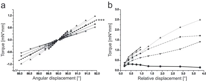
For all three legs, effectiveflexor tibiae moment arm length (0.564 mm) is twice that of the extensor tibiae (0.282 mm). Flexor tibiaefibres are 1.5 times longer (2.11 mm) than extensor tibiae fibres (1.41 mm). Active isometric force measurements demonstrated that extensor tibiae single twitch force is notably smaller than its maximal tetanical force at 200 Hz (2-6 mN compared to 100-190 mN) and takes a long time to decrease completely (> 140 ms). Increasing either frequency or duration of the stimulation extends maximal force production and prolongs the relaxation time of the extensor tibiae. The muscle reveals ‘latch´ properties in response to a short-term increase in activation. Its working range is on the ascending limb of the force-length relation- ship (see Gordon et al. (1966b)) with a shift in maximum force development towards longer fibre lengths at lower activation. The passive static force increases exponen- tially with increasing stretch. Maximum forces of 5 mN for the extensor, and 15 mN for theflexor tibiae occur within the muscles´ working ranges. The combined passive torques of both muscles determine the rest position of the joint without any muscle activity. Dynamically generated forces of both muscles can become as large as 50-70 mN when stretch ramps mimick a fast middle leg swing phase. FT joint torques alone (with ablated muscles) do not depend on FT joint angle, but on deflection ampli- tude and velocity. Isotonic force experiments using physiological activation patterns demonstrate that the extensor tibiae acts like a low-passfilter by contracting smoothly to fast instantaneous stimulation frequency changes. Hill hyperbolas at 200 Hz vary a great deal with respect to maximal force (P₀) but much less in terms of contraction velocity (V₀) for both tibial muscles. Maximally stimulated flexor tibiae muscles are on average 2.7 times stronger than extensor tibiae muscles (415 mN and 151 mN), but contract only 1.4 times faster (6.05^mm_s and 4.39 ^mm_s ). The dependence of extensor tibiae V0 and P0on stimulation frequency can be described with an exponential saturation curve. V0increases linearly with length within the muscle´s working range. Loaded release experiments characterise extensor and flexor tibiae series elastic components as quadratic springs. The mean spring constantβof theflexor tibiae is 1.6 times larger thanβof the extensor tibiae at maximal stimulation. Extensor tibiae stretch and relax- ation ramps show that muscle relaxation time constant slowly changes with muscle

history. High-speed video recordings show that changes in tibial movement dynam- ics match extensor tibiae relaxation changes at increasing stimulation duration.

Zusammenfassung

Um das Fortbewegungsverhalten eines Tieres verstehen zu können ist nicht nur die Kenntnis neuronaler Aktivität erforderlich, sondern auch die Umsetzung dieser Muster in Muskelaktivität. Die Stabheuschrecke stellt in Bezug auf die Erzeugung motoneu- ronaler Aktivität ein gut untersuchtes System dar. Diese motoneuronalen Aktiv- itätsmuster sind das Ergebnis des Zusammenspiels zwischen sensorischen Signalen, den zentralen neuronalen Netzwerken jedes Beingelenks und der Koordination der Beine untereinander. Die Muskeln des FT- (Femur-Tibia) Gelenks sind in ihrer Mor- phologie und der Art ihrer motoneuronalen Innervation beschrieben. Es ist jedoch wenig bekannt darüber, wie sich eine Stimulation ihrer Motoneurone in der Entwick- lung von Kraft oder Verkürzung ihrer Fasern widerspiegelt. Einer der beiden Muskeln, die das Gelenk bewegen, ist der Extensor tibiae, der sich für eine derartige Unter- suchung besonders gut eignet, da er nur drei Motoneurone besitzt, die simultan gereizt werden können. Dies kommt einem physiologischen Aktivierungsmuster recht nahe.

Sein Antagonist, der Flexor tibiae, ist komplizierter innerviert und eine biomecha- nische Untersuchung ist ausschließlich bei Rekrutierung aller Motoneurone sinnvoll.

welches mit der abgeschnittenen Muskelsehne verbunden wurde.

Beide tibiale Muskeln aller Beine wurden in Hinblick auf ihre Geometrie untersucht:

Die Muskellänge des Extensor tibiae ändert sich mit dem Cosinus des FT-Gelenkwinkels, die des Flexor tibiae hingegen mit dem negativen Cosinus, ausser bei extremen Winkeln (nahe 30° oder 180°). Bei allen drei Beinen ist die effektive Hebelarmlänge des Flexor tibiae von 0.564 mm doppelt so lang wie die des Extensor tibiae (0.282 mm). Flexor tibiae Fasern sind mit 2.11 mm anderthalb mal so lang wie Extensor tibiae Fasern (1.41 mm). Messungen der aktiven Muskelkraft zeigen, dass die Einzelzuckungskraft des Extensor tibiae deutlich kleiner ist als seine maximale tetanische Kraft bei 200 Hz (2-6 mN im Vergleich zu 100-190 mN) und dass sie lange braucht, um wieder voll- ständig abzufallen (>140 ms). Erhöhung entweder der Frequenz oder der Dauer einer Reizung verlängert die Dauer maximal erzeugter Kraft und verlängert die Relax- ationszeit des Extensor tibiae. Der Muskel zeigt ‘Latch´- Eigenschaften sobald es zu kurzfristigen Aktivierungserhöhungen kommt. Sein Arbeitsbereich befindet sich auf der aufsteigenden Flanke der Kraft-Längen-Beziehung (siehe Gordon et al. (1966b)).

Die Entwicklung maximaler Kraft ist bei niedriger Aktivierung zu größeren Faserlän- gen hin verschoben. Passive Kraft steigt mit wachsender Muskeldehnung exponen- tiell an. Innerhalb des Arbeitsbereichs treten maximale Kräfte von 5 mN beim Ex- tensor und 15 mN beim Flexor tibiae auf. Die kombinierten passiven Drehmomente beider Muskeln bestimmen den Ruhewinkel des Gelenks, der sich ohne Muskelak- tivierung einstellt. Dynamische passive Kräfte von Extensor und Flexor tibiae können 50-70 mN groß werden, wenn die Dehnungsrampen einer schnellen Schwingphase des Mittelbeins nachempfunden werden. Kräfte im Gelenk (also ohne Muskeln) sind unabhängig davon, welchen Winkel das FT-Gelenk beschreibt. Sie sind jedoch von der Amplitude und Geschwindigkeit tibialer Auslenkung abhängig. Der Extensor tib- iae verhält sich bei physiologischer Aktivierung wie ein Tiefpassfilter: er zeigt einen glatten Kontraktionsverlauf bei schnellen Änderungen instantaner Reizfrequenz. Hill- Hyperbeln beider tibialer Muskeln zeigen große Variabilität in Hinsicht auf maximal erzeugte Kraft (P0) aber variieren weit weniger in Hinsicht auf maximale Kontraktion- sgeschwindigkeit (V₀) bei einer Reizfrequenz von 200 Hz. Maximal gereizte Flexor tibiae Muskeln sind im Schnitt 2.7 mal stärker als Extensor tibiae Muskeln (415 mN und 151 mN), verkürzen sich jedoch nur 1.4 mal schneller (6.05 ^mm_s and 4.39 ^mm_s ).

Die Abhängigkeit von V₀ und P₀ des Extensor tibiae kann mit einer exponentiellen

Sättigungskurve beschrieben werden. V₀ wächst linear mit der Muskellänge inner- halb des Arbeitsbereichs. Durch Experimente, bei denen der Muskel abrupt entlastet wird, kann man die serienelastische Komponente von Extensor und Flexor tibiae als quadratische Feder charakterisieren. Die Federkonstante β des Flexor tibiae ist im Durchschnitt um den Faktor 1.6 größer als die des Extensor tibiae. Reizung des Ex- tensor tibiae mit Dehnungs- und Entspannungsrampen zeigen, dass sich die Zeitkon- stante der Entspannung langsam mit der Muskellänge ändert und daher dynamische Eigenschaften des Muskels langanhaltend von vorigen Muskellängenänderungen ab- hängig sind. Hochgeschwindigkeitsvideoaufnahmen zeigen, dass bei Steigerung der Reizdauer Änderungen der Dynamik tibialer Bewegung mit Änderungen des Relax- ationsverhaltens des Extensor tibiae einher gehen.

Contents

Abstract . . . 1

Zusammenfassung . . . 4

A. Introduction 11 B. Materials and Methods 21

2 Measurements with the Aurora 300B dual mode lever system . . . 25

3 Animal preparation and dissection . . . 27

4 Extracellular motoneuronal recording . . . 27

5 Electrical stimulation of motoaxons . . . 28

5.1 Recruitment of extensor tibiae motoneurons . . . 28

5.2 Physiological stimulation of extensor motoneurons . . . 32

5.3 Stimulation offlexor tibiae motoneurons . . . 33

5.4 Isometric force experiments . . . 33

5.5 Isotonic force experiments . . . 34

6 Photo and video tracking of tibia movements . . . 35

7 Data achievement, storage and evaluation . . . 36

7.1 Statistics . . . 36

C. Results 38

1.3 Moment arm determination . . . 41

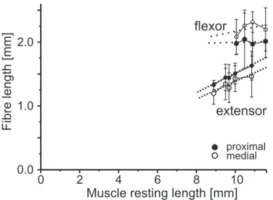
2 Fibre length measurements of middle leg tibial muscles . . . 42

3 Sarcomere length measurements of middle leg tibial muscles . . . 43

4 Femoral cross-sectional area . . . 48

C2 Force measurements in the isometric domain 49 1 Actively generated forces . . . 49

1.1 Single twitch kinetics . . . 49

1.2 Force kinetics at different activation . . . 52

1.3 Post-stimulational force dynamics at different activation . . . . 53

1.4 Post-stimulational force dynamics at different stimulation du- ration . . . 57

1.5 Force development in response to activation changes (latch) . . 58

1.6 The force-length relationship at different activation . . . 62

C3 Passive forces I 68 1 Stretch experiments . . . 68

1.1 Visco-elastic properties I . . . 68

1.2 (Static) passive force-length relationship . . . 71

1.3 Dynamic passive forces . . . 73

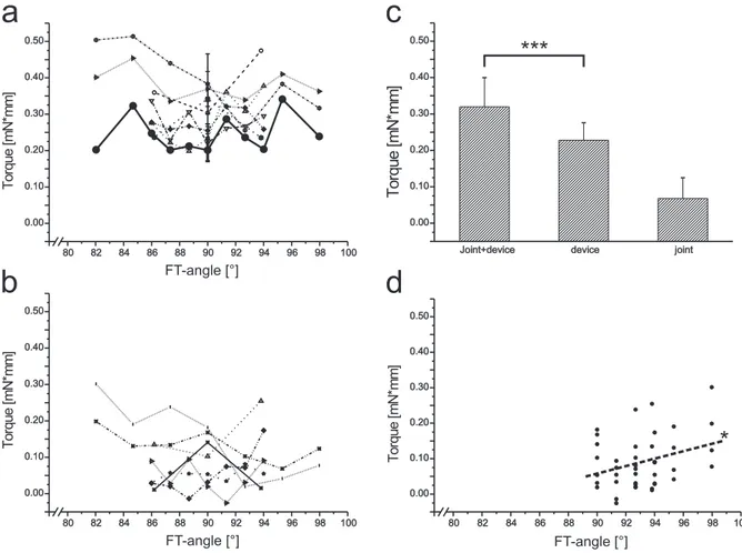
2 Significance for tibial movements . . . 76

3 FT-joint torques . . . 78

C4 Force measurements in the isotonic domain 84 1 Muscle contractions in response to physiological stimulation . . . 84

2 Loaded release experiments in response to tonical stimulation: the force- velocity relationship . . . 89

2.1 The Hill hyperbola at maximal stimulation . . . 91

2.2 Deviations from the hyperbolic shape . . . 95

2.3 The Hill hyperbola at different activation levels . . . 96

2.4 Activation dependent parameters . . . 97

2.5 Length dependence of the maximal contraction velocity . . . . 99

3 Isometric and isotonic contraction dynamics at different muscle lengths 100 C5 Passive forces II 105 1 Series elasticity . . . 105

1.2 Series elasticity of the extensor tibiae at different activation lev-

els . . . 108

2 Visco-elastic properties II: creep experiments . . . 109

C6 Force generation under naturally occuring FT joint movement patterns 116 1 Extensor tibiae forces before, during and after simulated stance phase 116 2 Extensor tibiae forces at the simulated transition from swing to stance phase . . . 122

3 Interaction of agonistic and antagonistic passively and actively gener- ated forces during simulated swing and stance . . . 126

3.1 Simulating tibial swing / stance phase . . . 126

3.2 Simulated swing relaxation at maximal tibia extension . . . 129

3.3 Simulated swing relaxation after hitting an obstacle . . . 130

D. Discussion 134

D2 Force measurements in the isometric domain . . . 142

D3 Passive forces I . . . 155

D4 Force measurements in the isotonic domain . . . 166

D5 Passive forces II . . . 182

D6 Force generation under naturally occuring FT joint movement patterns 188

Appendix 197

1.1 Sequencer scripts . . . 198

1.2 Analytical script . . . 204

Bibliography 205 Abbreviations . . . 220

List of Publications . . . 222

Acknowledgements . . . 225

Erklärung . . . 227

Curriculum vitae . . . 228

A. Introduction

INTRODUCTION

Locomotion can be described as the translation of the center of mass through space along a path requiring the least expenditure of energy (Inman (1966); Mochon and McMahon (1980)). In doing so, an organism´s nervous system is believed to represent a source of commands that are issued to the body as direct orders. However, rather than issuing direct commands, the nervous system can only make suggestions which are reconciled with the physics of the system and task at hand (Raibert and Hodgins (1993); Full and Farley (2000)). In terms of the integrated function of motor behaviour, the neural system and mechanical actuators rely heavily on each other´s properties as well as their organisation (Ettema and Meijer (2000)). As neural and muscular sys- tems coevolved, the activity of a motoneuron is likely to be tuned to the properties of the muscle it innervates in terms of its cellular properties for instance (Hooper et al. (2006)). Depending on their contraction dynamics, muscles can differ in their response to temporal components of the neural inputs they get (review in Hooper and Weaver (2000)). Prediction of movement from motoneuron spike activity alone is therefore impossible (Hooper et al. (2006)). Consequently, the combined knowledge about muscular properties together with the neural activity driving the muscle is nec- essary to describe appropriately how nervous systems generate motor output. Within the translation process of neuronal activity into movement, there are parameters on different organisation levels that can bear a high degree of complexity that needs to be considered. The number of motor units a muscle consists of (e.g. ∼150 in the cat soleusmuscle, Boyd and Davey (1968)) or the mechanics of power transmission (e.g.

the morphological arrangement of the stick insect retractor unguismuscle, Radnikow and Bässler (1991)) are just two examples for parameters that can vary a lot in terms of their complexity (e.g. cockroach extensor muscles 177 and 179 are innervated by a single excitatory motoneuron, Pipa and Cook (1959)). Beyond that, many kinds of behaviour require an organised interplay of several muscles or even muscle groups.

Some muscles feature the capacity to achieve context-dependent roles, like the poste- rior I1/I3/jaw complex inAplysia californica, that can mediate biting and swallowing by changing the direction of force it exerts (Neustadter et al. (2007)). Another example is the metathoracic second tergocoxal muscle (Tcx2) in the locustSchistocerca gregaria, which acts as an indirect wing levatoror as a coxal remoter (Malamud (1989); Mala- mud and Josephson (1991)). Muscles have the capacity to not only accelerate a mass, but also to avoid movements by braking or by resisting an external force (Hildebrand (1988)). Particular cockroach extensor muscles can operate as active dampers that only absorb energy during running (Full et al. (1998)) and stick insects can simultane-

ously exert braking and propulsive forces during part of each stride (Graham (1983)).

Hence, interpretation of the neuromuscular transform requires knowledge about the functional context a muscle is implemented in. For this reason, it is advantageous to study muscle biomechanics in a well investigated system in terms of the neural patterns occuring during the behaviour in focus. Concerning locomotion, such an or- ganism is the stick insect,Carausius morosus(Orlovsky et al. (1999); Büschges (2005);

Ritzmann and Büschges (2007)). The walking movement of its legs can be separated in two sections: stance and swing. During stance, the leg has ground contact and during swing, the leg lifts off the ground (Cruse (1985a;b)). A characteristic motoneu- ronal activity can be attributed to both phases in the walking animal (Graham (1985);

Büschges et al. (1994)). This motor output is the result of a complex interaction be- tween local sensory feedback, central neural networks governing the individual leg joints, and coordinating signals between the legs (e.g. Bässler and Büschges (1998);

Dürr et al. (2004); Büschges (2005); Gruhn et al. (2006); Borgmann et al. (2007)). The stick insect´s femur-tibia (FT) joint, which is the functional knee-joint of the insect leg, is particularly well described in lots of aspects. Early examinations dealt with the joint´s morphological organisation (Bässler (1967)). The motoneuronal innerva- tion patterns of the muscles moving the joint (Bässler and Storrer (1980); Debrodt and Bässler (1989; 1990); Bässler et al. (1996)), the extensor andflexor tibiae, and the motor output controlling tibia movement during walking (Bässler (1993a); Büschges et al.

(1994); Fischer et al. (2001)) are known, too. Some aspects of the control of these neu- ral patterns including the activity of the central premotor networks (Bässler (1993a);

Driesang and Büschges (1993); Büschges (1995b); Büschges et al. (2004)) were also revealed. In an attempt to relate specific sensory and neuronal mechanisms to the generation of the natural sequence of events forming the step cycle in a single leg, all previously collected knowledge was incorporated into the neuro-mechanical simula- tion of the stepping stick insect (Ekeberg et al. (2004)). However, the realisation of this simulation required not only the available information about neural activity but also the modelling of the simulated effectors, i.e. the muscles involved, byfixing the most important muscle physiological parameters defining them. At that time, those parameters were not yet measured. The search for information about ‘typical insect leg muscles´ led to the insight, that insect muscles can vary a lot in their properties (e.g. maximal force output). Especially the activation level of leg motoneuron pools during each locomotory duty cycle, i.e. how changes in motoneuron activity will af- fect muscle activation and thereby the movement amplitudes generated, shows large

INTRODUCTION

discrepancies between species. Fig. A.1 presents the comparison of motoneuronal firing patterns of muscles involved in locomotion in three insect species (the fruitfly Drosophila melanogaster, the cockroachBlaberus discoidalisand the stick insectCarausius morosus) during physiological movements. Flight muscle b1 depicted in A.1areceives one action potential per wing stroke, hindleg extensor 179 shown in A.1bis activated by three or four action potentials per locomotory cycle (during fast running), whereas the middle leg extensor tibiae shown in A.1c carries out a swing phase with more than 30 action potentials of the fast motoneuron FETi (mean spike number per burst, see Hooper et al. (2007a)). Each muscle is designed for maximal power and efficiency in its important range of speed (Full et al. (1998)). The control of activation, i.e. the properties of force production and contraction related to the motoneuronal spike fre- quency, varies a lot between muscles and suggests their individual twitch-to-tetanus ratios to be very different among the three species shown. This ratio represents an es- sential muscle physiological parameter that indicates a muscle´s capacity to finetune force and movement. The large differences in activation control between these three examplary species highlights the urgency of muscle physiological investigations in the stick insect.

Hooper and colleagues demonstrated that extensor tibiae motoneuronalfiring is highly variable (Hooper et al. (2006)). Measuring this variation on the effector level is the only way to tell whether this variation is really of physiological relevance for the animal. Given the well known neural aspects of stick insect leg motor control, under- standing of the FT-joint control would therefore be greatly increased by examining the biomechanics of the joint’s muscular system. Conveniently, the extensor tibiae represents a very suitable system for the investigation of muscle parameters: it is a pinnate muscle whose distal end is easily accessible by opening the femur with a few cuts and whose innervation is rather simple: one fast and one slow motoneuron (FETi and the SETi; Bässler and Storrer (1980)) and an additional inhibitory common in- hibitor motoneuron (CI₁; Bässler et al. (1996); Bässler and Stein (1996)), that run in a single nerve (nl3, Marquardt (1940)). Its antagonist, theflexor tibiae is very different in terms of its innervation. It features more than twenty-five excitatory (Goldammer et al. (2007)) and two inhibitory motoneurons (Debrodt and Bässler (1990)) that run in a single nerve as well (ncr, Marquardt (1940)). Especially in the case of the flexor tibiae, controlled extracellular stimulation of a particular set of motoneurons is diffi-

Figure A.1:Various forms of insect locomotion require different motoneuronalfiring patterns. aThe Mb1 motoneuron in Drosophila melanogaster spikes once every wingbeat cycle (modified from Heide and Götz (1996)). bThe metathoracic trochanter-femoral extensor muscle 179 of Blaberus discoidalis fires either three or four action potentials per running cycle (modified from Full et al. (1998)). cThe mesothoracic FETi motoneuron of Carausius morosus generates usually > 30 action potentials per swing phase (single middle leg preparation stepping on a treadwheel, see Fischer et al. (2001)).

cult to achieve and the physiological relevance of such a recruitment pattern unclear.

The number of possibilities in terms of motoneuronal activation patterns occuring in a behaviourly relevant situation is too large.

To overcome the difficulties of extracellular motoneuronal stimulation, thefirst tibial muscle force measurements were performed in response to movement of the chor- dotonal receptor apodeme, which acts as a feedback transducer measuring the angle between femur and tibia (Bässler (1965); Cruse and Storrer (1977)). The chordotonal organ is a position controller which works as a closed loop control system which en- ables the tibia to resist disturbance inputs (Bässler (1965; 1974); Cruse and Storrer

INTRODUCTION

(1977)). Extensor andflexor tibiae act as the actuators within the mechanism, as their forces try to resist the artificial disturbance input (Cruse and Storrer (1977)). Initial measurements were made from the tibia (Bässler (1974)) and later from the extensor and flexor tibiae muscles separately (Storrer (1976); Cruse and Storrer (1977); Bässler (1983)). The reason for the avoidance of extracellular motoneuronal stimulation was justified with concerns towards the order of recruitment of extensor tibiae motoneu- rons. FETi has the largest diameter (Bässler and Storrer (1980)) and is therefore the first one to be recruited at nl3 stimulation (for a detailed explanation, see Pearson et al. (1970); Stein and Pearson (1971)). Thus, extracellular SETi stimulation would always involve stimulating FETi as well, which was considered to be too far from a physiologically interesting situation and left the experimentators unsatisfied at that time. Consequently, measuring tibial muscle forces and length changes in response to direct motoneuronal stimulation was not taken into account.

However, a simultaneous extracellular stimulation of all extensor motoneurons comes actually quite close to a naturally occuring activation pattern. During walking, FETi, SETi and CI₁are activated maximally during swing phase of the middle leg (Schmitz and Hassfeld (1989); Büschges et al. (1994)). In this context, CI₁ activity switches off force production of dually innervated fibres (Bässler et al. (1996); Bässler and Stein (1996)). Depending on the walking situation, extensor motoneurons can also be ac- tive during stance phase before the initiation of swing, although at a reduced level (Graham (1985); Schmitz and Hassfeld (1989); Büschges et al. (1994)). Simultaneous stimulation of all three extensor tibiae motoneurons via nervenl3would therefore ab- solutely make sense and was chosen to be the right method to activate the extensor tibiae. Hence, by taking benefit of the knowledge available (see above), the middle leg extensor tibiae provides a lot of advantages that make it an ideal muscle physio- logical subject to study, which was done in the thesis at hand.

The muscle investigations presented in theResultssection required a careful selection of the most relevant questions that need to be answered to improve understanding of stick insect walking, as muscle physiology in general is a very broad and com- plex field. It ranges from molecular studies on e.g. ATP-driven Ca²⁺ -pump (Lou et al. (1997)) over force length measurements on highly specialised muscles that can be stretched nearly three times their resting length (Rose et al. (2001)) to the quantita-

tive description of the centre of gravity dynamics during the long jump take-off phase in humans (Seyfarth et al. (1999)). This thesis concentrates on the description of the main basic relationships that generally characterise a muscle and further deals with the interaction of characteristics and the development of individual parameters in a physiologically relevant context. The revelation of one of these basic characteristics, the so-called force-length relationship, was closely linked to the progressive explo- ration of structural processes within a sarcomere due to the development of tech- niques like electro microscopy. Those processes are summarised in the term ‘sliding filament theory´ (Huxley and Niedergerke (1954a); Huxley and Hanson (1954); Page and Huxley (1963)). A. E. Huxley and H. E. Huxley described the existence of cross- bridges as those structural elements, that are responsible for force generation and for the sliding of thick and thinfilaments (Huxley (1957a;b)). The biochemical processes involved were termed ‘power stroke´. Finally, the isometrically developed muscle forces at differentfibre lengths could be explained by the number of attached cross- bridges and are described by the sarcomere model (Gordon et al. (1966b)). In order to interpret this force-length relationship, previous knowledge about the muscle length change within the working range of the limb, which is supposed to be moved, is re- quired (Full et al. (1998)). This additional information is of particular importance as the muscle experiences length changes during every single contraction. Investigation of pinnate muscles like the extensor andflexor tibiae requires a further determination of thefibre length, as muscle length and fibre length are not the same, in contrast to parallelfibred muscles like e.g. the humanbiceps brachiimuscle.

Another important muscle characteristic is the force-velocity relationship, which rep- resents a fundamental property of the contractile system: the ability of a muscle to adjust its force to precisely match the load by varying the speed of shortening appro- priately (Edman et al. (1997)). Fenn and Marsh (Fenn and Marsh (1935)) were thefirst to describe this relationship that was a few years later characterised by a rectangular hyperbola (Hill (1938)). This Hill curve defines a muscle´s mechanical capacity - the maximum shortening velocity (V₀), the maximum stress (P₀) and the expected power output at any load less than P0or at any shortening velocity between 0 and V0 (Ed- man and Josephson (2007)). Hill provided evidence that muscle shortening involves heat production, which is due to inner friction that a muscle needs to overcome dur- ing shortening. The heat production by the muscle is proportional to the amount of shortening, that the muscle experiences. The Hill-equation describes the interrelation-

INTRODUCTION

ship between force, velocity and heat (Hill (1938)). Edman mentioned the possibility to use the force-velocity relationship as a relevant index of muscle activity (Edman et al. (1997)). Experiments on locustflight muscle (Schistocerca gregaria) showed that it was indeed possible to derive a so-called ‘degree of activation´ by releasing a muscle at different particular time points during a twitch (Malamud and Josephson (1991)).

This is in line with A.V. Hill, who found out that this was a good method to deter- mine when the muscle´s ability to develop work output peaks. Interestingly, this peak arises much earlier than the maximal isometric force output (Hill (1938)). In this con- text, computer models present good means to valuate the importance of a parameter in terms of comparing a situation where this parameter is implemented and another situation where it is ommited, as demonstrated by van Soest and Bobbert (van Soest and Bobbert (1993)). They could imposingly show the actual importance of muscle´s force-length and force-velocity characteristics in a human vertical jumping model and which sort of impact those characteristics have to a sudden perturbation. In general, muscle shortening represents a trade-off between the constraints of either moving fast or generating large power output. Elastic elements have the ability to uncouple muscle fibre shortening velocity from body movement to allow muscle fibres to op- erate more slowly, yet more strongly (Roberts and Marsh (2003)). Investigations on the plantaris longus muscle in the frog Rana catesbeiana reveals series elasticity to be essential to increase the mechanical work done in order to perform a fast and pow- erful movement at the same time (Roberts and Marsh (2003)). Passive elements like the series elasticity can have a major impact on locomotion behaviour. In the locust, passive torques have the capacity to lift even a loaded limb without any motoneuron activity: a large part of flexions and the initiation of extensions were attributable to passive forces (Schistocerca gregaria, Zakotnik et al. (2006)). The distribution of forces that arises during limb movement comprises not only the momentum of the actual mass that needs to be accelerated, but also the passive muscle forces of antagonistic muscle(s) and frictional joint forces, that have to be taken into account. The relevance of passive muscle forces scales with body size (Hooper et al. (2009)) and represents an essential movement and posture defining parameter in small animals like the stick in- sect. It was shown that loss of motoneuronal innervation in the extensor tibiae can be compensated (to some extent) by an increase in passive static tension, which can lead to a maintenance of walking behaviour (Bässler et al. (2007)). Thus, the knowledge about the neuromuscular transform represents only a part of the information that is needed to understand movement generation. Musculoskeletal units, leg segments,

and legs do much of the computations on their own by using segment mass, length, inertia, elasticity, and dampening as ‘primitives´ (Full and Farley (2000)). A mechani- cal system can react much faster to perturbations during rapid, rhythmic activity (Full and Koditschek (1999)). Nonetheless, passive dynamic control lacks the plasticity of active neural control, since suites of integrated structures which have evolved over millions of years take longer to modify (Full and Farley (2000)).

In addition to the questions that arise around the activation of a muscle and its passive behaviour, one crucial aspect of the above mentioned musculoskeletal units is their relaxation behaviour after active contraction. That is, a muscle can still exert force even though motoneuronal firing has ceased. In the isotonic force domain, the stick insect extensor tibiae takes on average 52 ms after a burst to start relaxing (Hooper et al. (2007a)). This becomes especially functionally relevant at step transitions, when a muscle´s relaxation has notfinished and the antagonist muscle is about to be acti- vated. In the stick insect, the transition from swing to stance features co-contraction in terms of an extensor andflexor tibiae activity overlap (single leg preparation inCuni- culina impigra, Fischer et al. (2001)). Antagonistic muscle co-contraction attributable to long muscle time constants facilitates substantial load compensation (Zakotnik et al.

(2006)). The joint stiffness, that results from co-contraction, represents an important part of a successful control strategy. The level of co-contraction can vary with the history a muscle has experienced in terms of its previous activation or previously happened muscle length changes (see e.g. Ettema and Meijer (2000); Herzog et al.

(2003); Ahn et al. (2006)).

The investigations in this thesis are presented and discussed in six chapters respec- tively. The stick insect FT joints of front-, middle- and hindleg were examined in re- spect to their geometrical characteristics. In the middle leg, femur and muscle cross- sectional area, fibre length and sarcomere length were determined for the extensor andflexor tibiae. Experiments determining statically and dynamically generated pas- sive forces and testing creep behaviour were conducted on both tibial muscles of the middle leg as well. The middle leg extensor tibiae was investigated in respect to its twitch and tetanus kinetics, its relaxation dynamics at different activation levels, its latch properties and its force-length characteristic in the isometric domain. Ex- periments in the isotonic domain included force-velocity measurements at different

activation and length levels, the contraction behaviour in response to physiological input and series elasticity measurements at different activation levels. In the final part, the interaction of characteristics and the relaxation behaviour were investigated by mimicking physiologically occuring extensor muscle length changes. Video track- ing of tibial movement should test whether the change in extensor tibiae relaxation dynamics after different activation durations is reflected in tibia movement. Due to the large amount of motoneurons, active middle legflexor tibiae measurements were restricted to quick release experiments including the calculation of the parameters P0 and V0 and series elasticity determinations. Theseflexor nerve stimulations were exclusively conducted at maximum activation (i.e. entire motoneuronal recruitment and maximum stimulation frequency). The role of FT joint forces alone was examined by ablating both tibial muscles and deflecting the joint.

Some of the data shown in this thesis (parts of chapters C1, C2, C3, C4 and C5) were already published in Guschlbauer et al. (2007) (FT joint geometry of all legs, mid- dle leg extensor tibiae single twitch and force-length relationship in terms of actively generated isometrical force and passive static tension, extensor tibiae Hill curves at different activation and maximal shotening velocities at differentfibre lengths, exten- sor tibiae series elasticity at different activation). Other data shown (a part of chapter C3) are about to be published in parts of Hooper et al. (2009), where I appear as a con- tributing author (extensor andflexor tibiae passive static tension,flexor tibiae dynam- ically generated passive tension, joint deflections either intact, with muscles ablated or with joint tissue ablated). Some further measurements presented (a part of chapter C4) were the basis for the analysis shown in Hooper et al. (2006; 2007a;b), where I also appear as a contributing author (physiological stimulations of the extensor tibiae in the isotonic force domain).

B. Materials and Methods

MATERIALS & METHODS

Experiments were carried out on adult female stick insects of the species Carausius morosus Br. from a colony maintained at the University of Cologne. Animals were kept under artifical light conditions (12 h darkness, 12 hours light) and were fed with blackberry leaves (Rubus fructiosus). 10 sturdy-looking animals of the same size as used in the experiments had an average body length of 77.1 ± 2.28 mm and average weight of 940 ± 70 mg. All experiments were performed under daylight conditions (setup light, Olympus) and at room temperature (20-22°C).

1 Femur, muscle, fibre and sarcomere length measurements

The extensor andflexor tibiae muscles were exposed for length measurements by cut- ting a small window into the proximal and distal part of the femur. The red-coloured autotomal ring (Schindler (1979); Schmidt and Grund (2003)) was assigned as proxi- mal end. Parts of the main leg trachea, the chordotonal organ and thefirst of three re- tractor unguis muscles (Radnikow and Bässler (1991)) were cut off and highly diluted

‘Fast Green´ (Sigma) was applied in most cases. Muscle length was calculated under the microscope by determining the distance from the insertion of the most proximal fibre to an orientation mark (see Fig. B.1, shown for the extensor tibiae) and adding the distance from this mark to the insertion of the most distalfibre into the tendon.

The animal´s abdomen was stimulated tactilely several times during a test series to make sure that the investigated muscle was tensed throughout (Bässler and Wegner (1983)). The tibia was moved on a plastic goniometer from 30° (maximally flexed) to 180° (maximally extended) and length measurements were taken in 10° intervals.

This range (150°) is considered as the maximum working range of both tibial muscles (Storrer (1976); Cruse and Bartling (1995)). 90° was defined as the FT-joint angle at which both muscles are at their resting length for the stick insect (Friedrich (1932);

Storrer (1976)) and for Blaberus discoidalis(Full et al. (1998); Ahn and Full (2002)). Fe- mur cross sectional area was detemined by cutting middle legs on the level of the mid-coxa. Sections of approximately 1 mm thickness were cut from the medial part of the femur with a razor blade (Rotbart).

Fibre length measurements were performed on musclesfixed in situ using 2.5% glu- taraldehyde in phosphate buffer pH 7.4 (Watson and Pflüger (1994)) with the joint at the 90° position and the entire femur opened laterally. The animal was again stimu- lated tactilely several times duringfixation (see above). Fibres were pulled from the proximal and medial parts of the femur because in these locations both muscles are primarily innervated by fast motoneurons (Bässler et al. (1996); Debrodt and Bässler (1989)). Muscle length changes and fibre length measurements were done using a 20x magnifying oculometer (Wild-Heerbrugg) at 25x magnification, femoral length was determined at 6x magnification. Calibration was done with a aluminium-ruler (estimated accuracy of 0.005 mm).

Two different methods were used measuring sarcomere length. In a first approach, middle leg FT-joints were set at angles of 30°, 90°, or 180°. The specimens werefixed in a mixture of 13% formaldehyde/ 59% ethanol/ 6% glacial acetic acid and embed- ded in paraffin. 15µm thick sagittal slices were made and stained with the fast Nissl procedure (Burck (1988)). Sarcomeres were visualised under a light microscope with a polaroidfilter and measured with the analySIS software (Soft Imaging System, Olym- pus). The second approach consisted in staining extensor and flexor tibiae muscles with phalloidin (Phalloidin-FluoProbe 647H 650/670 nm) after fixing the femur as a whole in a mixture of 4% paraformaldehyde in 0.1 M sodium phosphate buffer (pH 7.4) and separating the muscles carefully afterwards from the femoral tissue. Phal- loidin was dissolved in 1.5 ml methanol which results in a 6.6 nmol/ml phalloidin so-

proximal end of the femur

proximal end of the

extensor tibiae distal end of

the femur orientation mark

30°

90°

180°

Trochanter Coxa

Femur

Tibia

Figure B.1:Schematic representation of the geometrical arrangement of the femur-tibia joint in the stick insect middle leg. See text for details.

MATERIALS & METHODS

lution. 7.5µl of this solution were mixed with 400µl phosphate buffered saline (PBS).

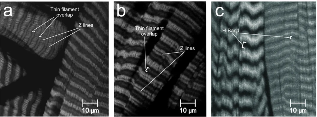
Muscles were incubated in a mixture of 0.16 ^nmol_ml phalloidin solution with 1% Triton- X in PBS for 15min (modified from Thuma (2007)). Concentrations of 0.32 ^nmol_ml and 0.08 ^nmol_ml were tested as well and led to worse results. Phalloidin stained sarcomere lengths werefirst measured at the actual contraction state when beingfixed, that is at 30° and 180° FT-joint angle. Then, sarcomere lengths were determined by standardis- ation according to the instructions suggested by Thuma (2007), see Fig. B.2. The goal of such a normalisation procedure is to specify lengths independent from contraction state, because different muscles are known to have different sarcomere lengths. The comparison of sarcomere lengths between muscles therefore necessitates the reduc- tion of a sarcomere to its own physical characteristics. This reduction provides an unambigious anatomical base to determine sarcomere length independent from con- traction state, because the standardised sarcomere length measures two times thin filament length.

Figure B.2:Standardisation of sarcomere length. Sarcomere lengths from the same type of muscle differ because of different muscle contraction states. To correct this, a standardisation protocol can be applied to each sarcomere length (modified after Thuma (2007)).

2 Measurements with the Aurora 300B dual mode lever system

The ‘Aurora 300B dual mode lever system´ (Aurora Scientific Inc, Ontario, Canada) is a device enabling to measure and control both force and position simultaneously and to make the transition from force to position control with only small transients (Fig.

B.3 shows a picture of the device). Forces of maximally 500 mN and length excursions of maximally 10 mm can be detected with a force signal resolution of 0.3 mN and a length signal resolution of 1 micron. Force step and length step response time are 1.3 ms and 1 ms respectively. It acts like a length controller that is precision force-limited and acts exclusively as a force controller if an external load attempts to pull harder than the set force level. Its servo motor has a preferred direction of force application although forces can be measured in both directions. Load should be attached to the lever arm such that a muscle contraction will pull the lever arm in a counterclockwise direction (when viewed from the shaft end of the motor).

The lever arm of the Aurora servo motor is 30 mm long and perforated at the tip.

Its connection to a muscle is the combination of an u-shaped pin being glued to a cut thick insect pin being in turn glued to a 0.1 mm thin hook-shaped insect pin. A few experiments were done using a sterile silk thread (50 µm; Resorbi, Nürnberg) in combination with a hook-shaped insect pin as link between lever arm and muscle.

Force and position measurements with the lever system were mainly made on the extensor tibiae muscle of the middle leg, some experiments dealt with theflexor tibiae muscle´s properties. The lever system was tuned so that length control was critically damped and inertia compensation was adjusted to minimise force transients using triangle waveforms as suggested in the Aurora´s instruction manual.

For investigation of FT joint torques, a special lever arm was built (mechanics depart- ment of the Zoological institute, University of Cologne). Its effective moment arm length is 4.75 mm. The lever arm that was usually used narrows to the perforated tip and has an effective moment arm of 30 mm. A middle leg was cut on level of the mid- coxa and wasfixed on the platform and positioned such that its FT joint rotational axis and its pivot was the same as the servo motor´s. A plastic rod formed the connection between the lever arm and the tibia, with which it could be easily attached because

MATERIALS & METHODS

Figure B.3:The Aurora dual-mode lever arm system 300B (Aurora Scientific Inc.). The picture shows only the main device, i.e. the controller, not the servo motor.

of a notch that was sligthly narrower than the average stick insect tibia (see Fig. B.4).

Additionally, a drop of super glue (Loctite, Uhu Alleskleber) assured a good bond between tibia and the notch in the plastic rod. Finally, apodemes of both extensor and flexor tibiae were cut through the soft cuticle at the anatomical transition from femur to tibia withfine scissors.

c a

b

Figure B.4:Measuring FT-joint torques with a specialised device. atibia,bfemur embedded in dental cement,cmodified lever arm (the lever arm that was usually used is depicted in Fig. B.7).

3 Animal preparation and dissection

All legs except one middle leg were cut at the level of the mid-coxa. The animal was treated according to the established procedures and was fixed dorsal side up on a balsa wood platform so that the tibia of the remaining leg was suspended above the edge of the platform in all extensor tibiae investigations. The tibia had to be cut in allflexor tibiae experiments. Coxa, trochanter, and femur were glued to the platform with dental cement (Protemp II, ESPE, St. Paul, MN, USA). The distal end of the femur was opened carefully to ensure that as many musclefibres were left intact as possible.

The femoral cavity wasfilled with ringer (NaCl 178.54 mM, HEPES 10 mM, CaCl₂7.51 mM, KCl 17.61 mM, MgCl₂25 mM) (Weidler and Diecke (1969)) several times during each experiment (see also Becht et al. (1960)). Muscle investigations were achieved by inserting the hook-shaped insect pin (described above) through the cut distal end of either the extensor orflexor tibiae distal muscle apodeme (see also Ahn et al. (2006)).

Cutting of the apodeme was conducted under controlled conditions: muscle length was set to its corresponding length at a FT-joint angle of 90° at the beginning of each measurement. Flexor tibiae muscles were normally that strong that the hook-shaped pin had to be glued (Loctite 401, Uhu Alleskleber Super) to the apodeme in addition to the insertion through the tendon.

4 Extracellular motoneuronal recording

Nerves F2 and nl3, both containing the three extensor tibiae motoaxons, were recorded in different experimentsen passant(Schmitz et al. (1991)) with a monopolar hook elec- trodefilled with silicone paste (high-viscosity, Bayer), modified by the mechanics de- partment of the Zoological institute, University of Cologne. Afine polyethylene tube can be slided on the nerve, which can in turn be isolated with the silicone paste. A silver wire (0.25 mm in width) served as a reference electrode. The signal was either preamped with a battery-powered optocoupler (100x) or by a ‘Ultra low noise pream- plifier MA103´ (50x), boosted by an AC-filter amplifier (20x or 50x) and sampled by an AD-converter (Cambridge Electronics 1401) with 12500 Hz. The filter range settings of the booster were usually 150 Hz-9500 Hz.

Nerve activity could be made audible by a monitor (1278), that was amplified with a DCfilter amplifier (1274A). All devices were built in the electronics department of the

MATERIALS & METHODS

Zoological insitute of the University of Cologne when not noted differently.

5 Electrical stimulation of motoaxons

5.1 Recruitment of extensor tibiae motoneurons

Most experiments were done on the extensor tibiae muscle because it is innervated by only three motoneurons (Bässler and Storrer (1980)), all of which have their axons in nervenl3(nomenclature according to Marquardt (1940)). After opening the thorax dorsally and removing the gut, fat, and connective tissue to expose the mesothoracic ganglion, a bipolar hook electrode was placed under nerve nl3 (Marquardt (1940)).

The nerve was crushed proximally with a foreceps and isolated with white vaseline (Engelhard Arzneimittel GmbH & CoKG, Niederdorfelden). In order to measure ei- ther the tension or the muscle length change of the middle leg extensor tibiae, the axons of its innervating motoneurons, the FETi, SETi, and CI₁ were stimulated via a stimulation isolation unit putting out current (‘Universal stimulus isolator Model 401´). Due to their differing axon diameters (Bässler and Storrer (1980)), the three motoneurons can be sequentially activated by increasing stimulation strength; FETi has the lowest threshold (Fig. B.5 a(i) and a(iiii)), SETi the next highest (Fig. B.5 a(ii) and a(iiii)), and CI₁ the highest (Fig. B.5 a(iii) and a(iiii)). The determination of the appropriate current pulse amplitude to use in the nerve stimulation was complicated by a conflict between 1) the desire to routinely stimulate all three motoneurons (FETi, SETi, and CI₁) and 2) the desire to keep the current amplitude low enough that the nerve could be repeatedly stimulated over long periods without damage. This issue was even more difficult to resolve because the dissection required to allow extracel- lular recordings from the extensor nerve F2 in the distal femur close to the muscle (which is required to test whether all three axons are being stimulated) inevitably damaged some more distal musclefibres which are mostly dually innervated (Bässler et al. (1996)) and also added considerable time to the dissection procedure. It was con- sequently not possible to both perform the long experiments on undamaged muscles and to check if all three motoaxons were being stimulated in the same preparation.

To overcome these difficulties, 15 experiments were performed using a dissection en- abling to record extracellularly from the F2 nerve, where the relative thresholds of the three motor units were measured. Since these experiments were also short, forces

could be measured that the muscle produced as the number of stimulated nerve units changed (due to the inevitable musclefibre damage, in all cases less than the usually detected forces reported in the Results part). Infive of these experiments stimulating the nerve at 1.5 fold the threshold for visible twitches resulted in reliable stimula- tion of all three motor axons. In eight experiments, stimulation at this level was not sufficient to reliably activate the two smaller fibres (typically SETi but not CI₁ was reliably activated). However, increasing the stimulation amplitude in these experi- ments showed that (presumably because FETi induces by far the largest twitches, and because in most of these cases SETi was already being activated at the 1.5 stimulation level), when a sufficient stimulation amplitude was achieved to activate the other two units completely, this induced negligible changes (in 7 preparations none, in one 3%) in muscle force production. Fig. B.5 b(i)-(iiii) shows forces and F2-recordings in re- sponse to a 50 Hz stimulation pulse train of a representative experiment. In Fig. B.5 b(i), 75% of the pulses excited FETi and 25% FETi and SETi. In In Fig. B.5 b(ii)„ 50%

of the stimuli elicited FETi and 50% FETi, SETi and CI₁. Fig. B.5 b(iii), shows re- cruitment of all three motor units with every pulse, doubling the current amplitude in Fig. B.5 b(iiii), shows no further increase in force. In the remaining two experi- ments stimulating the additional two units resulted in an increase in muscle force of 20±4%. These experiments also showed that stimulating the motor nerve with cur- rent pulses 1.5 times larger than the visible twitch threshold for long periods of time did not induce any sign of nerve damage (e.g., an increase in stimulation failures).

These control experiments thus showed that in 90% of preparations stimulating nl3 with a current amplitude 1.5 times greater than the FETi threshold either resulted in activation of all three motor axons or, if not, that the failure to activate SETi and CI₁completely had a negligible effect on muscle force production. In the remaining 10% of preparations, the lack of the SETi and CI₁ only induced a modest decrease in measured muscle force. These observations led to the decision to simply set the amplitude of the current pulses to approximately 50% above threshold generating a visible twitch (Malamud and Josephson (1991)). Pulse trains of different frequencies could be either applied with a SPIKE2 sequencer program or with a ‘Universal digital stimulator MS501´ triggered by a SPIKE2 sequencer script in intervals of at least 30 seconds to assure inter-trial muscle recovery. Pulse duration was 0.5 ms in all exper- iments (Josephson (1985); Stevenson and Josephson (1990); Malamud and Josephson (1991); Full et al. (1998); Ahn and Full (2002); Ahn et al. (2006)).

MATERIALS & METHODS

FETi

stimulus artefact

1 T

1.78 T

2.67 T

5.33 T 1.33 T

FETi, SETi

1.78 T FETi, SETi, CI₁

1.5 T

a(i) b(i)

a(ii) b(ii)

a(iii) b(iii)

a(iiii) b(iiii)

50 ms 0.5 mN

100 ms

10 mN

*

**

***

5 ms

* ** ***

Figure B.5: Isometric forces induced in the middle leg extensor tibiae muscle by electrical stimula- tion of nerve nl3 with different current amplitudes. In all panels the top trace is a stimulus monitor (note pulse height changes as stimulus amplitude was increased), the second trace is an extracellular recording of nerve nl3, and the third trace is muscle force. a(i)-a(iii)show sequential recruitment of FETi (a(i)), FETi and SETi (a(ii)) and FETi, SETi and CI1 (a(iii)) recorded in extensor leg nerve F2 in response to single stimuli. a(iiii): An enlarged version of the recordings showing the sequential addition of new units. 1 T was 0.0023 mA.b(i)-b(iiii) show F2-recordings and forces in response to a 50 Hz pulse train. In b(i), 75% of the pulses excited FETi and 25% FETi and SETi. Inb(ii), 50%

of the stimuli elicited FETi and 50% FETi, SETi and CI1. b(iii)shows recruitment of all three motor units with every pulse. Doubling the current amplitude (b(iiii)) induced no further increase in force.

In this experiment the SETi spikes were of larger amplitude than FETi spikes. This is uncommon and likely because nerve F2 was recorded very distally in the femur. In all panels the electrical disturbance in the nerve recording that coincides with the stimulus is a stimulus artifact, not an action potential (arrow ina(i)).

Figs. B.6 (scheme) and B.7 (photograph) summarise the above described. All experi- ments examining muscle force were based on this setup configuration.

Position

OFFSETIN OUT

Force

OFFSETIN OUT

Current

a b

c

d e

f g

Figure B.6: Experimental overview. a Computer, b AD-converter, c stimulation isolation unit, d bipolar electrode on either nerve nl3 (extensor tibiae stimulation) or ncr (flexor tibiae stimulation), e monopolar recording electrode on nerve F2,fAurora servo motor,gAurora control device.

MATERIALS & METHODS

a b

c

d

Figure B.7: Photo showing the setup for all experiments dealing with muscle force and/or muscle length. abipolar hook electrode stimulating either nl3 or ncr,bmonopolar hook electrode,recording F2 (used in 15 control experiments)ccombination of an insect pin glued to a thin hook-shaped insect pin inserting either the end of the cut extensor orflexor tibiae tendon,dlever arm being part of the Aurora servo motor (black).

5.2 Physiological stimulation of extensor motoneurons

Physiological stimulation of the extensor muscle could be achieved by initially record- ingnl3activity with a monopolar hook electrode while the right middle leg of a stick insect performed step-like movements on a treadband (N=1, see Fig. B.8). For a de- tailed description of the single leg preparation see Fischer et al. (2001). The treadband consisted basically of crepe paper being driven by two engines (Gabriel et al. (2003);

Gabriel (2005); Gabriel and Büschges (2007)). On each engine axis, a plastic cylinder was mounted. On of the two engine was used as a tachometer to enregister treadband velocity. These recordings were further analysed by sorting out FETi motoneuron ac- tion potentials with the SPIKE2 software, marking those as events and using them as triggers to stimulate nervenl3(see above) of a different animal. Muscular output was exclusively investigated in the isotonic domain setting the force output on the servo motor manually as high that total muscular relaxation between the putative step-like

movements (visible as contractions) could be accomplished.

7.4cm/s

1 s

nl3 activity Treadwheel

velocity

Figure B.8:Recorded extensor nerve (nl3) activity while a stick insect performed step-like movements on the treadwheel shown in the lower trace (for a detailed description of the single leg preparation, see Fischer et al. (2001)). Velocity of the treadwheel´s tachometer is displayed in the upper trace.

5.3 Stimulation of flexor tibiae motoneurons

The flexor tibiae muscle is innervated by about 14 motoneurons running in nerve

ncr (Storrer et al. (1986); Debrodt and Bässler (1989); Gabriel et al. (2003)). Recent investigations resulted in an even larger number of flexor tibiae motoneurons (18- 27, N=8; Goldammer et al. (2007)). Thus, extracellular stimulation of this muscle is complicated to achieve, therefore only a few experimental paradigms carried out on the extensor tibiae were conducted on the flexor tibiae as well. A bipolar hook electrode was placed under nerve ncr, crushed proximally and isolated with vaseline (as described for nervenl3). At the beginning of each experiment in the isotonic force domain, stimulation amplitude was increased until isometric force showed no further increase and force development showed no visible stimulation failure. Sequential recruitment was mainly tested investigating single twitches. As maximal output by the MICRO1401 A/D converter (Cambridge Electronic Design Limited; Cambridge, UK) was limited to 5 V (i.e. maximally 250 mN force application on the Aurora´s lever arm), the force output was amplified with an amplifier / signal conditioner MA102 by factor 2 (500 mN is the Aurora´s maximal measuring capacity). Detected flexor tibiae forces were not exceeding this value.

5.4 Isometric force experiments

Experiments to determine the active and passive force-length characteristics accord- ing to Gordon and colleagues (Gordon et al. (1966b)) were carried out as follows:

MATERIALS & METHODS

muscle length was manually set to a FT joint angle of 90° at the beginning, defined as the muscle´s resting length l₀ (see above). It was then released 0.75 mm (0.5 l₀) and subsequently stretched in coarse steps (mostly 0.15 mm) with sequencer-generated ramps of 0.05 ^mm_s up to 0.75 mm beyond the muscle´s resting length (ca. 1.5 l₀). In a different approach, the focus was on examining force development within the mus- cle´s working range using small ramps (0.05 mm) within the range of ca. 0.8 l₀ to ca. 1.2 l₀ to obtain a more accurate screening. Actively generated forces were inves- tigated with a paradigm of different stimulation frequencies at each length position after having relaxed. For isometric force experiments, the influence offilament over- lap on force generation was examined by stretching the muscle in ramps of different size over a range of 1.5 mm using a SPIKE2 sequencer script (see Appendix). The stimulation protocol was carried out at each muscle length.

5.5 Isotonic force experiments

Force-velocity curves (Hill-curves) were obtained according to the established pro- cedures (Edman et al. (1976); Edman (1979; 1988); Malamud and Josephson (1991);

Edman and Curtin (2001)). For isotonic force experiments, the influence of load on contraction velocity and muscle series elasticity was determined by application of different force levels on the lever arm during tetanus using a SPIKE2 sequencer script (see Appendix). Extensor muscles were stimulated to reach steady-state contraction under isometric conditions and then allowed to shorten under isotonic conditions against a variety of sequencer-generated counter force levels. Lengthening of the muscle was accomplished with stretches while applying sequencer-generated load levels larger than the tetanical steady-state contraction force.

Caution was taken that the variation of tetanical steady-state force before the switch to force control (for a given stimulation frequency) was not exceeding 15% for all contractions used for further data evaluation (see also Ahn et al. (2006)). The big- ger the difference between tetanical force (P0) and force level applied, the more the muscle went bad (observed in numerous experiments). Therefore, experiments were generally designed the following way: load levels were applied rather randomly be- tween 0.25P₀and 1P₀, load levels < 0.25P₀were applied at the end of an experiment.

Switching from force to length control involved a sudden increase in force applied on

the lever arm. This abrupt step was most often filtered with an ‘amplifier / signal conditioner MA102´ or a ‘DCfilter amplifier 1274A´.

6 Photo and video tracking of tibia movements

Movement still photographs of the FT joint were taken in two different ways. Passive movements were tracked by pinching cut middle legs horizontally into a clamp (with- out gravitational effects). A digital camera (Fuji FinePix S602) was placed on a tripod above the leg´s FT joint. Pictures were evaluated using the CorelDRAW software:

cursors could be tilted to the desired angle in order to lay on top of the tibia picture in focus with an estimated accuracy of 1°. Muscles were ablated by cutting the tendon at the most distal part of the femur without previous dissection, the transitional part from femur to tibia has a very thin cuticle and is well accessible.

Tibia movement dynamics were tracked using a VGA highspeed camera (‘AVT Mar- lin F-033C´) and pictures were taken in 10 ms intervals. Nerve stimulation (200 Hz pulses) of eithernl3(extensor tibiae) orncr(flexor tibiae) and video tracking were trig- gered by a ‘Universal Digital Stimulator MS501´. The antagonistic nerve (eithernl3or ncr) was crushed or cut to avoid reflex behaviour (Bässler and Büschges (1998)). Each frame was triggered individually by a 100Hz pulse train that was gated manually.

Nerve stimulation started with a 50 ms delay to have at least 5 single pictures of the non-moving tibia as a reference point. Pictures were evaluated in CorelDRAW in the same way described for the photos taken with the digital camera ‘Fuji FinePix S602´

(see Fig. B.9).

Figure B.9:(a)Single still photographs of a tibia movement high-speed video track with the FT-joint highlighted with red lines at the leftmost picture. The example shows stimulation with 80 spikes.

Angular evaluation of the asterisk marked picture is displayed in(b): FT joint angle was measured by setting cursors in the CorelDRAW software.

MATERIALS & METHODS

7 Data achievement, storage and evaluation

Data was recorded on a PC using a MICRO1401 A/D converter with SPIKE2-software (both Cambridge Electronic Design Limited; Cambridge, UK). The stiffness of the measuring system was measured by connecting the insect pin directly to the base of the platform. It was greater than 7500 ^mN_mm and can therefore be neglected in our mea- surements. Jewell and Wilkie discuss the influence of the compliance of the measuring device thoroughly (Jewell and Wilkie (1958)). For most of the data analysis, custom SPIKE2 script programs were written (see Appendix). Plotting, curvefitting, and er- ror evaluation were performed in ORIGIN 6.0 (Microcal. Software Inc, Northampton, MA, USA) except for the RC-type growth and exponential decay fits performed in GNUPLOT. This PhD-thesis was written with the LYX/L^ATEX software.

7.1 Statistics

Mean values were compared using ORIGIN´s either unpaired

t=^{!(x1−x2−d0)}

s²(_n¹

1+_n¹

2)

or paired

t=^D_S^−d0

D

two sample t-test.

(xn is mean of samplegroup n, d₀ is a specific value, s is the S.D., nn is number of samplegroup n, Dis the mean difference.)

Regression analysis was used to determine linear correlation between two variables.

The ORIGIN 6.0 software used the least squares method to calculate the slope and provided the correlation coefficient (R value) and the p-value (probability, that R=0).

Means, samples and correlation coefficients were regarded as significantly different from zero or each other atp<0.05. The following symbols show the level of statistical

In the text, N gives the number of experiments or animals while n gives the sample size. All data were calculated as mean ± S.D. R-values or R²-values are specified additionally when it was reasonable.

C. Results

C1 Femoral geometry

The ‘Results´ part is generally structured in the following way: the majority of the thesis´ topics were examined on the extensor tibiae of the middle leg, some of those topics were also examined on theflexor tibiae of the middle leg. Muscle data is there- fore presentedfirst for the extensor tibiae and subsequently for theflexor tibiae when ever there was data collected. Front, middle and hind leg data are presented, when available, for both muscles when indicated.

1 Muscle length measurements of front, middle and hind leg tibial muscles

1.1 Relationship between resting muscle length and femur length

Resting muscle length was measured (at 90° joint angle, see ‘Materials and Methods´) offlexor and extensor tibiae for the front (flexor N=3, extensor N=3), middle (flexor N=5, extensor N=8) and hind legs (flexor N=3, extensor N=3, Fig. C.1). The linear regression of this data showed in 5 cases a significant dependence of muscle length on femur length (*, p < 0.05 or better), only theflexor tibiae front leg data showed no significant dependence. The dependence was simplifed in Fig. C.1 for all legs to a pure proportionality forcing the regression lines through the origin (dotted lines, see also Tab. C.1). For comparison, the 1:1 proportion (solid line) is included.