Institute for Biological Physics

(1)

Institute for Biological Physics

University of Cologne

Master Thesis

The Fitness Landscape of Translation

Written by Mario Josupeit

Supervisor: Prof. Joachim Krug

Second revisor: Prof. Andreas Schadschneider

Cologne, 07.08.2020

(2)

(3)

1. Introduction

In this thesis I examine the fitness effects in the translation step of protein synthesis.

The idea for this topic originates from the surprising findings of Zwart et al. in 2018 [35].

Their paper on the TEM-1 β-lactamase gene of the Escherichia coli bacterium states, that synonymous mutations, which are those mutations, that change the nucleic acids, but leave the encoded protein the same, can have a strong fitness effect, with the fitness being the number of offspring per individual. The fitness in an environment with the antibiotic cefotaxime, was measured for all combinations of 4 synonymous mutations in the TEM-1 gene. This fitness is the antibiotic stress resistance IC99.99. The synonymous mutations observed are at the 9th, 17th, 87th and 89th codon of the gene that has a length of 284 codons. The space of all 2⁴ possible combinations of mutations is called a fitness landscape, connecting a point within the mutations landscape to the measured fitness.

The fitness landscape of synonymous mutations from Zwart et al. [35] features many neutral mutations, which do not change the fitness, as well as sign epistasis, a feature of the landscape where the effect of a mutation has a different sign on different backgrounds. The key to analyzing and understanding such a landscape, beyond looking at the fitness values themselves, is to examine interactions of mutations in the landscape. This work presents a tool for analyzing these landscapes which could lead to a deeper understanding of the characteristics of synonymous mutations. The goal of this thesis is to formulate a model for interacting mutations and analyze the landscape that inspired this investigation. The road to this goal reaches from the biological basics and the TASEP, a non-equilibrium physics model of translation, via the description of a model proposed by this thesis and comparisons to numerical results and literature, to an analysis of experimental results for a fitness landscape of synonymous mutations. The methods of this thesis reach from analytic approaches to numerical simulations and data analysis.

(6)

2. Biological concepts

All living cells use proteins, which makes protein production one of the most basic and essential parts of life. Proteins are the tools of the cell and can have various shapes, sizes and functions. Proteins are long chains of amino acids and are in most cases constructed by the cell itself. For each protein produced by the cell, there is a gene in the genetic code that determines the composition of the amino acid chain. The composition determines the function of the resulting protein. The genetic information is stored as triplets of nucleic acids, the codons. The process of protein production is called thecentral dogma of molecular biology, a term coined by Crick in 1970 [2]. This "dogma" states that the genetic information of the gene, stored as part of the cell’s DNA (deoxyribonucleic acid) is transcribed into a mRNA (messenger ribonucleic acid) and then translated by a ribosome into an amino acid chain, which then folds into the functional protein. One mRNA strand can have many protein producing ribosomes on it at the same time, but they can only move in one direction without overlapping and need to read all information of the gene before the protein is completed. This step of protein production has a large amount of processes associated with it and much of the cells functions are designed to enable this process.

Translation, the construction of new proteins by ribosomes, has three steps.

1) Initiation: A ribosome attaches to the mRNA and starts the translation by adding the first amino acid to the chain that will become the protein in the end.

2) Elongation:The ribosome moves along the mRNA and attaches one new amino acid to the amino acid chain for each codon.

3) Termination: Upon reaching one of three stop codons, the ribosome detaches from the mRNA and the amino acid chain detaches as a new protein from the ribosome.

2.1. Redundant amino acids

Amino acids are attached to the end of the produced protein, according to the sequence of codons on the mRNA. Each codon is translated into exactly one amino acid, or is a stop codon. The stop codon marks the end of the gene and therefore signals that the protein is fully produced.

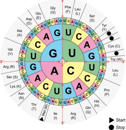
Each codon consists of three nucleic acids, leading to 4³=64 specific codons, cf. figure 2.1.

Many of these possibilities are redundant, meaning that multiple codons code for the same amino acid. This redundancy is the reason why up to six different codons encode each of the 21 canonical amino acids. Codons that code for the same amino acid are called synonymous

(7)

2.1 Redundant amino acids

Figure 2.1.: The mRNA codons with their respective amino acids. Note that only the start codon methionine (labeledMet (M) in the figure) and tryptophane (labeledTrp(W)) are encoded by a single codon. The other amino acids have synonymous codons which encode them.

Graphic sourcehttps://de.m.wikipedia.org/wiki/Datei:Aminoacids_table.svg, vis- ited 25th of July 2020, licensed as free to use (Public domain).

[22]. When first discovered, it was believed that synonymous codons have no effect on protein production, because they do not alter the sequence of amino acids in the protein.

More recent experimental findings [35] show a large change in the features of cells after exchanging codons with their synonymous counterparts. The synonymous substitution, i.e.

the exchange of one synonymous codon for another, keeps the sequence of amino acids the same. There exist examples for different speeds at which different synonymous codons are read during elongation [31, 18]. This different translation speed can lead to changes in protein stability and production yield [21]. Exploring this phenomenon is very interesting since this is a new angle from which researchers can understand protein production.

(8)

2.2 Mutations and synonymous mutations

2.2. Mutations and synonymous mutations

Mutations are exchanges, deletions or insertions of genetic material in the genetic code of an organism. This means that a mutation changes the genetic code and sometimes a feature of the cell. The effects of mutations can be various. The protein encoded by the gene may change its structure and stop working or, in a rare, but better case for the cell, the protein gains a new feature that is beneficial for the cell. The new feature caused by a mutation can be anything from a metabolic function to the disabling of an important protein leading to the cell’s death. If there is a measurable change, the phenotype of the cell changed. The concept of phenotypes is explained in very large detail by Taylor in chapter 6 of [30]. It is important to note, that the effects of a mutation may be beneficial or disadvantageous. Especially if there is no competition between individuals, for example because the individuals never interact with another, less efficient individuals also grow well and produce offspring. For experiments on bacteria, the solution is often diluted so much, that all individual bacterial colonies are the offspring of one ancestor each.

In the following sections I often use the termsign of a mutation, where the sign is positive, if the mutation is beneficial, and negative if it is disadvantageous. Difference in genetic code is used as a measure for distance betweengenetic species. The more nucleotides differ from one genome to the other, the further they are away from another. the members of one genetic species are all individuals in a population, that share the exact same genetic code [1], which is a more rigid definition of the term species. This also means that mutations change one genetic species into another. The term species is only defined for sexually reproducing organisms and not to be confused with the term I use in this work.

In this thesis, I focus on synonymous mutations. This is a special case, where codons are changed in such a way, that the amino acids they code for stay the same. Even though there is no change in the protein sequence, there are interesting effects on the phenotype [22]. This is an example for effects on the phenotype of an organism beyond changing its amino acid sequences. A feature that changes when a synonymous mutation happens is the elongation rate of the changed codon. The elongation rate is the rate at which the ribosome translates a codon and is an essential factor for the organisms fitness, which is explained in the next section.

(9)

2.3 Fitness and fitness landscapes

2.3. Fitness and fitness landscapes

Fitness is a macroscopic variable dependent on the genome of the individual. The genome is the collection of all information encoded by the genes of an organism. It gives a single macroscopic value dependent on many microscopic values, similar to the free energy of a gas or the color of a crystal. It is described as a function of the full genome and the living circumstances of the organism. It is impossible to define a fitness without knowing the environment of the organism. In the most simple case, one can find certain proteins that are the most important for the survival of the cell. In the example study referenced multiple times in this thesis by Zwart et al. [35] the E. coli bacteria grow in a medium with a high antibiotic concentration, which is why they need to produce a certain protein, which deactivates the antibiotic, or die. The fitness F(⃗ν) of this organisms then is highly dependent on the codon sequence ν⃗₀ = (ν₁, ν₂, ...ν_L) of length L of the gene that can deactivate the antibiotic. The fitness is then F( ⃗ν₀) = F₀. A mutation m₁ changes the nucleic acid sequence at position x₁. This could be a point mutation exchanging only one nucleic acid, or a insertion or deletion of a section in the gene. The important sequence change for this thesis is the single exchange of one amino acid, which is also the most common mutation, which is why in the following only one rate and one position is taken into account at a time.

m₁∶ ⃗ν₀↦ ⃗ν₁ (2.1)

The new genome is then ν⃗₁= (ν₁, ν₂, ..., ν_x^′

1, ν_x₁₊₁, ...ν_L) and may exhibit a different fitness

F( ⃗ν0) ≠F( ⃗ν1) . (2.2)

A visualization of the fitness values and also the genomic distances is the fitness landscape.

It consists of different genomes mapped to their associated fitnesses. Two points in this space represent two different genetic species and are connected via mutations that change one genetic species into the other. Because each visualization shows different features of a fitness landscape, there are many ways of visualizing it.

Some common visualizations are the fitness plotted against the number of mutations and the N-dimensional hypercube.

The fitness plotted against the number of mutations shows the distance from the original genetic species. The original species is called the wildtype. The distance is the number of mutation steps that need to be taken to get from the wildtype to the other mutants. It is

(10)

2.3 Fitness and fitness landscapes

most commonly used to show that a landscape is very smooth or very rough, because this feature of the landscape is visualized very well. An example for fitness potted against the number of mutations can be seen in figure 2.4.

The fitness landscape can also take the form of an N-dimensional hypercube, where N is the number of different mutations of the organism [6]. This structure spans an N-dimensional space of edge length 1 (so each site can either be mutated or not mutated), with the 2^N fitness values at the corners of the hypercube. This visualization is most commonly used to show the pathways along which mutations can get from one point in the landscape to another. The fitness values themselves are less prominent in this visualization. Many examples of this visualization can be found in chapter 5 and in the example 2.2. The general form of this hypercube has four values on each edge. These four values correspond to the four nucleic acids that can be at those edges. It is common practice though to use a binary alphabet if there is only a maximum of one mutation at each position on the gene observed. The fitness landscape is easier to display with only two points on each edge.

F₀ F₁

F₂ F₁₂ m₁

m₁

m₂ m₂

Figure 2.2.:A two-dimensional fitness landscape displayed as a hypercube. Each direction in the landscape is one mutation. In the upper left corner is the unmutated wildtype fitness, that is the fitness of the original genetic species. Arrows point to the nodes of higher fitness.

As an demonstration example I choose F₀<F₂ <F₁₂<F₁.

Both visualizations can show how mutations interact, which is a main focus of this thesis and explained in the next section on epistasis.

There are many parameters that can be treated as the fitness of an organism. Whether it is the resistance to an antibiotic, if the cell grows in a medium with antibiotics, the ability to process more nutrients, if there is a new source of energy available, or the time it takes for an individual to produce offspring. All of those measures lead to reproductive success and can be a proxy for fitness. That is why, in evolution, fitness means reproductive fitness according to Wright [33]. This is the amount of offspring of one particular genetic species in the next generation, which is the definition of fitness used in this thesis.

(11)

2.4 Epistasis

2.3.1. Neutral mutations

If a mutation has no effect on fitness, it is called neutral (or silent). Displayed similarly to figure 2.2, figure 2.3 shows two cases of neutral mutations. In figure 2.3a, the mutation m₂ is always neutral. In figure 2.3b, the mutation m₂ is only neutral, if the mutation m₁ happened before it. Both cases do exist in nature. Displayed as a fitness landscape with the fitness plotted against the number of mutations, neutral mutations are lines without a slope, also called "flat". I use this to describe mutations in chapter 5. The case from figure 2.3b is further discussed in the next section 2.4, which explains epistasis.

F₀ F₁

F₂ F₁₂ m₁

m₁

m₂ m₂

(a)The 2-dimensional hypercube displaying a fully neutral mutationm₂ as thick blue lines.

This shows, that F₀=F₂<F₁ =F₁₂.

F₀ F₁

F₂ F₁₂

m₂ m₂

m₁

(b) The same landscape as before, but here, m₂ is only neutral if the mutation m₁ happened before. The ordering of the fitness values isF0<F2 <F1=F12.

Figure 2.3.

2.4. Epistasis

The effect of mutations often depend on the genetic background, i.e. all other information encoded by the genome of the organism. A very intuitively accessible example is a bacterium that develops both the ability to gather a new food and separately the ability to digest it.

This bacterium could develop both traits independent from another, but the large benefit only exists if both traits are present in the same bacterium at the same time.

This very important concept for this thesis is called epistasis. It describes the interaction of mutations. There are many different definitions for epistasis depending on the aspect of interest. The definition that I use states that epistasis is the change on the effect of one mutation m₂ due to the presence of another mutation m₁, described on page 667 in Crow and Dove’s book [3]. This definition can also be applied for interactions between more than two mutations. In the previous section there are some examples for (non-)epistatic landscapes. Figure 2.3a shows no epistasis, figure 2.3b shows epistasis in the mutation m₁, because the effect of m₁ is either neutral or beneficial, depending on the presence or

(12)

2.4 Epistasis

absence of mutation m₂ and figure 2.2 shows the special case of sign epistasis, where the presence of mutation m₁ changes the sign of the effect of mutation m₂ compared to the case where mutation m₂ acts on the wildtype. The definition for the terms sign epistasis and non-epistatic follow in the subsections 2.4.1 and 2.4.2.

2.4.1. Sign epistasis

A special case of epistasis is sign epistasis. It describes the change of one sign of a mutation dependent on the presence or absence of another mutation. This non-monotonic effect is very interesting, because two positive effects may produce a negative effect in conjunction or two negative effects may be beneficial together. Weinreich explains, that the sign of a mutation is under epistatic control [32].

If F₀ is the fitness of the unmutated wildtype species with genome ν⃗₀, F₁ is the fitness after mutation m₁ on the genome ν⃗₀ took place, turning it into ν⃗₁. F₂ is the fitness after mutationm₂ emerged on ν⃗₀ and F₁₂ is the fitness with both mutations present. The effect of mutation m₁ on the background ν⃗₀ is equal to the fitness difference F₁−F₀. The effect of m₁ on ν⃗₂ is equal to the fitness difference F₁₂−F₂.

(b)

0 1 2

Fitness

Number of mutations F₀

F2

F_1,2 F₁

(a)

0 1 2

Fitness

Number of mutations F0

F₂ F_1,2 F₁

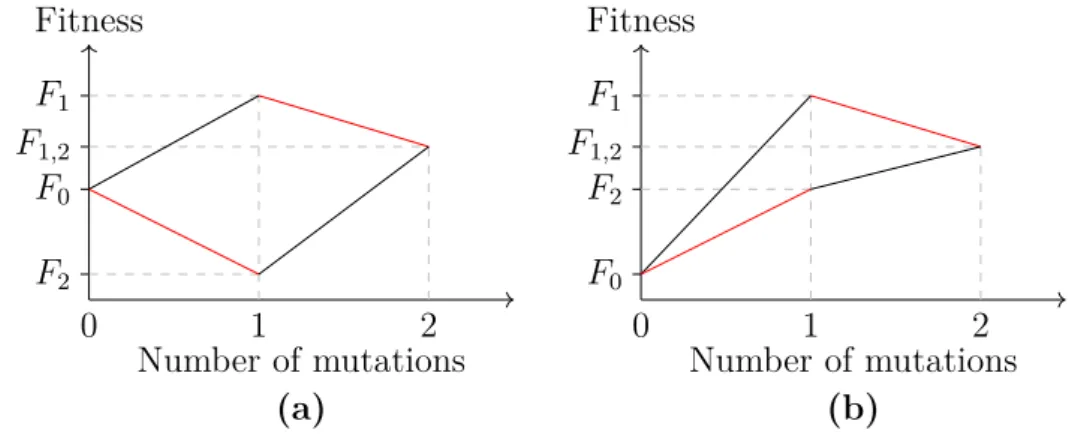
Figure 2.4.:The epistatic effects of two interacting mutations.(a): An example landscape with monotonic fitness effects, i.e. no sign epistasis. Mutationm₂ (red lines) always has a negative effect andm₁ always has a positive effect on fitness. The angles of the mutations change slightly, depending on the presence of the other mutation, but the sign does not change. (b): Non-monotonic system exhibiting sign epistasis. m₂ (red lines) has a positive effect only if m₁ is not present.m₁ itself does not display sign epistasis with respect to m₂ because it always has a positive effect whether m₂ is present or not.

If the difference between the fitness values without the mutationm2 being present(F1−F0) and withm₂,(F₁₂−F₂), have different signs, the presence of the mutationm₂ changes the

(13)

2.4 Epistasis

sign of the effect of the mutation m₁. Therefore if either or both E₁ ∶ (F₁₂−F₁)(F₂−F₀) <0

E2 ∶ (F12−F2)(F1−F0) <0 (2.3)

are true, the presence of one mutation flips the sign of the effect of the other.

Because the definition allows for either one of the equations or both to be true, drawn as a hypercube this sign epistasis shows up as antiparallel arrows. In the example 2.2, (F₁₂−F₁)(F₂−F₀) <0 is true and therefore the arrows associated with the m₂ mutation are antiparallel. In the example 2.4b, the mutationm₂has a positive effect, when it emerges on the wildtype (F₂ >F₀), but has a negative effect when the mutationm₁is already present (F₁₂<F₁). This can be seen in the different sign of the slopes of the red lines in example 2.4b. The example 2.4a does not feature this effect.

Sign epistasis is very interesting since one mutation can have a very large impact on the effect of another mutation. It not only changes the effects strength, but even whether the effects is positive or negative for the organism and the effects are not constant.

For this thesis sign epistasis is important, since the experimental fitness landscape by Zwart et al. [35] displays many cases of sign epistasis.

2.4.2. Non-epistatic case

In the non-epistatic case mutations are independent. Therefore the fitness effects are ad- ditive. In contrast to the epistatic case, the fitness effects of each mutation is constant.

If

F₁₂−F₂ =F₁−F₀ (2.4)

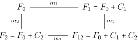
is true, there is no epistasis betweenm2 andm1. Transforming equation 2.4, it is equivalent to F₁₂−F₁ =F₂−F₀. Therefore both mutations have a constant effect on fitness and are independent form each other. Depicted as a hypercube of two dimensions this is shown in figure 2.5. The signs of the mutational effects C₁ and C₂ are not important for equation 2.4 to hold, therefore the strength of the effect remains constant. The effects C₁, C₂ can have positive or negative signs.

(14)

2.4 Epistasis

F₀ F₁ =F₀+C₁

F₂=F₀+C₂ F₁₂=F₀+C₁+C₂

m1

m2 m2

m1

Figure 2.5.: A fitness landscape with constant mutational effects C₁, C₂.

(15)

3. TASEP

In this thesis, I simulate ribosomes movement on the mRNA with the totally asymmetric simple exclusion process (TASEP) model, which is a well established model for protein synthesis and a standard model in the area of non-equilibrium physics. It was suggested in 1968 by MacDonald and Gibbs [20] and is also used for simulating other transport processes like traffic jams [23] and myosin movement (e.g. [8, 12, 15, 20, 19, 26]). Even though the kinetics of the TASEP are simple, it displays very interesting effects, such as spontaneous shock formation, phase transitions and edge effects. The phases of a TASEP and the fluctuations that occur within them during simulations are the topic of a paper by de Gier and Essler [9] in the context of solid state physics. For traffic models, all of these effects are easily observed in real scenarios, for the biological process that sparked the idea, there are many obstacles to the observation because most ways of measuring the parameters of the motion in the system require the system to be stopped from working.

Knowledge about the macroscopic observables of the TASEP system are important to gain an understanding of the mechanics of it, these are explained in section 3.2.

3.1. General TASEP mechanics

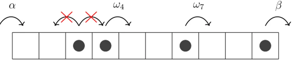
The TASEP exists on a one-dimensional lattice of length L on which particles move uni- directionally. The particles are subject to hardcore interaction, so they can not overlap or overtake another. They move from left to right taking steps, respectively jumps, of distance 1 along the one-dimensional system. These jumps occur between the sites and reflect the one elongation step of the ribosome. After entering at the left end with jump rate α they traverse the system at rates (ω₁, ω₂, ... , ω_L−1) = ⃗ω, which are the L−1 jump rates between all L sites in the system. The particles exit on the right, from site L, with jump rate β. The jump rates determine particle movement, given there is an empty space to the right of them. At its starting position the system is connected to an infinite reservoir of particles, so there is always a particle able to fill the first site. At the exit it is connected to a particle sink, so a particle at the last site can always leave the system [34].

α ω₄ ω₇ β

Figure 3.1.: Schematic representation of the allowed movement in a TASEP of length 10.

Particles enter at rate α on the left, move at their local rate and can not jump backwards or occupy the same spot as another particle. They leave the system on the right at rate β.

(16)

3.2 Measures in the TASEP system

3.2. Measures in the TASEP system

For the TASEP the interesting macroscopic parameters are the stationary current J, the stationary average density ¯ρand the travel time ¯τ. In the following I describe their general formulation. There is an exact solution for the homogeneous case in section 3.3. These parameters change when bottlenecks are present, explained in section 3.6.1. There is also an approximation for the current and density for random systems with a low initiation rate α by Szavitz-Nossan et al. [28] which is the topic of section 4.2.

3.2.1. Density

The local density ρ_i in the steady state, i.e. the system after is has relaxed for a sufficient time, is the likelihood to find a particle at position i. Its average across the system

¯ ρ=∑^L

i=1

ρ_i

L (3.1)

is a measure for the average amount of particles in the system. Even though it has been used as a measure for fitness, this density does not measure fitness. This is mostly used in experiments where ribosome profiling, which is a method where ribosomes are used to shield mRNA, is performed to measure the density of ribosomes. This misconception is often based on the idea that ribosomes move simultaneously, or the assumption that translation is only limited by α, which is a setup that has, according to my knowledge, not been observed in an biological system. If the density of ribosomes is high, the cell has less ribosomes available, costing energy, and the protein production yield does not increase as described in more details by Plotkin and Kudla in the section on measurements in their paper [22].

Closely related to the density is the average hole density, which is the likelihood to not find a particle at position i, which is simply 1−ρ_i.

3.2.2. Current

The current J in a TASEP is generally a function of all rates ω_i. There is no general solution for it, but at any moment in time, it can be understood as the rate at which the average particle in the system moves. This definition does not give an analytic formula for the current though, because in an inhomogeneous system, the rates at which the particle leave their sites is highly variable. In large homogeneous systems it can be approximated

(17)

3.2 Measures in the TASEP system as the product of the average density with the average hole density,

J =ρ¯(1−ρ¯) . (3.2)

The current can be approximated by the maximal permitted currentJ_ω_min through the site with the lowest rate ω_min.

In the case of protein production, the average current is a measure of how much protein is produced per mRNAstrand per unit time and therefore an often used measure for fitness.

3.2.3. Travel time

The travel time T as formulated by Szavits-Nossan and Evans [29], is a measure for the time it takes a particle from the first position in the TASEP to leaving the system. The travel time is the sum of the local densities of particles ¯ρ divided by the current J. This thesis uses a slightly different formulation, because I approach the topic of travel time from another direction, but the definitions are equivalent. The difference from the one in the paper by Szavits-Nossan and Evans is due to them starting to count at the second site, while I start at the first, which is why I multiply byL instead ofL−1 and that I focus in the average travel time per site ¯τ. The travel time T is

T = Lρ¯

J . (3.3)

The time that a ribosome spends at each site i is τ_i =ρ_i

J , (3.4)

and the average time that a ribosome spends at a site is

¯ τ = ρ¯

J . (3.5)

In the context of translation, the travel time is a measure of the time it takes one ribosome to produce one protein. Each particle encounters other particles with the probability ¯ρ. So if there is more jamming in the system, then the travel time is longer. The inverse of the travel time _τ¹_¯ is the translation efficiency. It is the rate at which proteins are produced per ribosome and is another measure for the fitness of an organism.

(18)

3.4 Three phases of the homogeneous TASEP

3.3. Homogeneous TASEP

The TASEP is called homogeneous if the jump rates for all sites are homogeneous,

ω₁ =ω₂ =...=ω_L−1=∶ω . (3.6)

There are three free parameters in all homogeneous TASEP systems, the initiation rate α, termination rateβ and the homogeneous elongation rate ω. The rates are only relative to an arbitrary time measure and the results are the same after renormalizing with α^∗ =

α

ω and β^∗ = ^β_ω, which is why any homogeneous ω can be set to 1 after rescaling. The homogeneous TASEP has been analytically solved by Derrida et al. and the stationary current and density are known [4, 5]. The following section 3.4 sums up the results for the homogeneous TASEP.

3.4. Three phases of the homogeneous TASEP

The homogeneous TASEP system separates into three phases, the low density (LD), high density (HD) and maximum current (MC) phase. The phase transition between the high density and low density phase is called the shock phase (cf. figure 3.2a).

If α is smaller than 0.5 and β is larger than α, the system is in the low density phase. α is the rate limiting factor for ribosome movement. For this case, the termination rate β is not a current limiting factor, because the density ρ in the system is always lower than the rate at which ribosomes exit from the last site. The rates in the bulk do not limit the movement because they allow J_{M C} = 0.25, the rate of the last site allows Jlast site=β(1−β)

and the current through the start site is α(1−α), which is smaller than the other two.

Therefore the density in the system is α. This leads to a lower density than in all other systems, hence the name low-density phase (LD).

If β is smaller than 0.5 and α is larger than β, the system has a very high density. In contrast to the low-density phase the current is limited by the termination rate β. The density in this system is 1−β, because particles leave the system at rateβ, and the density that remains at the last site and the traffic jam propagates to the left is 1−β. The system supplies more particles than can exit and is in a phase of high density (HD).

The third phase is the maximum current phase (MC). If a sufficient amount of particles can enter and leave the system. The entry and exit no longer limit the travel in the system.

This is true if the entry rate α ≥ 0.5 and the termination rate β ≥ 0.5. In this case, the

(19)

3.4 Three phases of the homogeneous TASEP current in the bulk is now rate limiting, because it reaches its maximum of 0.25 (cf. figure 3.2b). The density ¯ρ is 0.5 in the whole phase.

β

α

0 0.2 0.4 0.6 0.8 1 0

0.2 0.4 0.6 0.8 1

LD

HD M C

Shock Phase

(a) The phase diagramm for the homogeneous TASEP. It splits into three phases, high density (HD, lower right), low density (LD, upper left) and maximum current (MC, upper right).

The boundary between high density and low density is the shock phase (red), where the two bordering regions coexist.

J

¯ ρ

0 0.2 0.4 0.6 0.8 1 0

0.05 0.1 0.15 0.2 0.25

LD HD

M C

(b) The connection between the currentJ and the average density ¯ρ. On the left of the peak is the LD phase, on the right the HD phase. The line in the middle signifies the MC phase.

3.4.1. Phase boundaries

At the intersection between the phases, phase transitions occur. Between the low-density and the maximum-current phase and between the high-density and the maximum-current phase, there are second order phase transitions. The low-density system fills with particles asαincreases until it reachesα=0.5, where the bulk can no longer support a higher current and the maximum current phase is reached. The opposite is true for the high-density phase, here the density decreases as β increases until it becomes a maximum current system at β=0.5.

The phase transition between the low density phase and the high density phase is different.

Here the system approaches the lineα=βfrom either the low-density or high-density phase.

There it enters the shock phase, in which the system splits into a low-density part at the start and a high-density part at the end. The two phases coexist, because the particle enter at the same rate as they leave, so the system neither fills up nor drains. The particles enter

(20)

3.4 Three phases of the homogeneous TASEP

at a low rate and have almost no other particles in their way, due to the low density in the first part of the system, so they reach the intersection between the two parts rather fast.

At the other end of the system, the particles leave at a low rate, leading to a traffic jam in front of the termination end. As soon as there is a vacant spot at the last site, due to the high density at the end, this new hole is transported to the right very fast. The intersection between the phases is called a shock, due to the sudden change in density.

The shock diffuses through the system. Whenever a new particle arrives at the shock, the shock moves towards the start of the system, whenever a hole reaches the shock, it moves towards the end. This diffusion leads to a towards the end of the system linearly increasing average densityρ_i (cf. figure 3.3).

3.4.2. Edge effects

In general TASEP systems there are always edge effects. The density at the borders decays into the system. If the system is in the maximum current phase, this decay is a power law.

If the system is in the low-density or high-density phase, it decays exponentially. These changes in density is completely relaxed, there are tails at the boundaries like in figure.

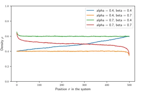
In the homogeneous TASEP, the larger the initiation rate α is, the stronger are the edge effects close to the start site. The sites close to the start display a density that is larger than the density in the center of the system if α≥β. A similar effect can be observed at the end of the system for β≥α, where the density drops. This is visualized in 3.3.

(21)

3.5 Inhomogeneous TASEP

0 100 200 300 400 500

Positionσin the system 0.0

0.2 0.4 0.6 0.8 1.0

Densityρ

alpha = 0.4, beta = 0.4 alpha = 0.4, beta = 0.7 alpha = 0.7, beta = 0.4 alpha = 0.7, beta = 0.7

Figure 3.3.: Example runs for the homogeneous system. The graphic shows the distinct characteristics of each phase. In the shock phase (blue) the density is monotonically increasing. In the high/low density phase (green/orange), edge effects are visible at the start/end and the system has the same overall density otherwise. In the maximum current phase (red), the density is on average at 0.5 and has tails at both ends.

Edge effects exist at all rates bordering different rates within the system as well and depends on the difference between the rates. Therefore this effect can also be observed in the bulk of inhomogeneous systems, because not all rates ω_i are the same. Other features of the inhomogeneous TASEP are explained in the next section 3.5.

3.5. Inhomogeneous TASEP

A synonymous mutation can change the elongation time of the affected codon and therefore the rate at that site. From experiments it is known that the change in the rates due to synonymous mutation can differ by a factor of up to 4 [31, 18]. These different rates have to be reflected in the simulations. The inhomogeneous TASEP reflects, that the rates ω_i of different sitesi, can have different values.

Unfortunately, in contrast to the homogeneous TASEP, these systems are not solved. The only analytical solution is an approximation for systems that have one very small rateαor ω_iby Szavits-Nossan et al. [28]. Therefore numerical simulations are required to understand these systems. Even for relatively small finite systems, there is no general solution and

(22)

3.6 Bottlenecks

numerical solutions are required to understand their behavior.

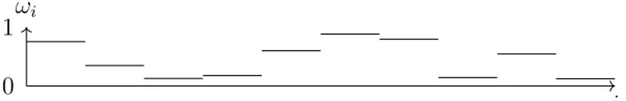
3.5.1. TASEP systems with random jump rates

The first approach to simulating a system of many free parameters is generating a system with random rates. These systems have large statistical noises, which do not abate, even at long timescales. The causes for the noise are edge effects throughout the system, that exist whenever different rates border another.

ω_i

i 1

0

Figure 3.4.: An example of a random landscape with random rates ω_i.

3.6. Bottlenecks

A second approach to understanding the TASEP using numerical simulations is to start from the analytically solved homogeneous TASEP with α =1 and β =1 and replace one of the jump rates ω_i at position x in the system with a rate r that is smaller than the other rates. This local inhomogeneity is called a bottleneck. The density in systems with a bottleneck acts similar to a fixed shock, but in contrast to the shock phase, it does not diffuse in the system and the density at the start of the system is high, and at the end of the system is low. Properties of bottlenecks are nicely explained by Schadschneider, Chowdhury and Nishinari in chapter 6 of their book on transport systems [23].

In this section, I make statements that are true for large systems (L>>1). The discontinuity in the rates leads to a fixed density behind the bottleneck and another fixed density before the bottleneck. I only consider large systems in the following, because the parameters bottleneck raterand density after the bottleneckρcan be used interchangeably, cf. section 3.6.4. The bottleneck is fully characterized by its position x in the system and rate r and therefore in the limit of large L, it can also be characterized by the density after the bottleneck and the position. The bottleneck rateris easier to use in numerical simulations, but has no explicit meaning in the context of fitness, because the exact relation between fitness and the rate is unknown and the density has a meaning connected to fitness, but can not be used as an input parameter in simulations. The exact function ρ(r) is not known for finite systems, but can be numerically calculated. This is done in section 3.6.4.

(23)

3.6 Bottlenecks Janovski and Lebowitz approximate the current J and density ρdepending on bottleneck rate r [13] and give an expansion for these values for finite systems [14]. Szavits-Nossan uses a matrix formulation of the transitions to calculate these functions up to the third order in the lowest rate in the system [27].

3.6.1. Measures in the TASEP with bottlenecks

The measures explained in section 3.2 change in a system with bottlenecks. A single bottleneck in an otherwise homogeneous system separates it into two parts, where each are themselves a homogeneous TASEP. The bottleneck reduces the density behind it and increases the density before it. In large systems, local inhomogeneties around the bottleneck in the density profile can be ignored because the density behind the bottleneck is mostly dependent on the raterof the bottleneck. In the following I assume the system to be large to have parameters that are more sensible for the model.

The average density of the second part of the system depends on the raterof the bottleneck (cf. figure 3.10). Because all particles have to travel through both parts of the system, the current of particles is

J =ρ(1−ρ) (3.7)

everywhere in the system and the density ρ is mainly dependent on the bottleneck rate.

Equation (3.7) has two solutions for ρ ∈ (0,0.5), therefore the average local density after the bottleneck ρ_after needs to be equal to the average local density of holes before the bottleneck 1−ρ_before (cf. figure 3.5), the average density of particles before the bottleneck and after the bottleneck add up to 1. For ease of notation I define

ρ∶=ρ_{af ter} , (3.8)

⇒ρbef ore=1−ρ . (3.9)

There is a similarity to the shock phase, described in section 3.4.1, because the system is separated into two parts by the bottleneck, one high-density phase and one low-density phase, but the shocks in bottleneck systems do not diffuse through the system like in the shock phase, but are fixed.

The position of the bottleneck in the system is given by x∶= i

L∣

ωi=r , (3.10)

(24)

3.6 Bottlenecks

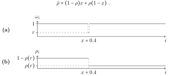
which is a value between 0 and 1. For a bottleneck with rater at sitei in a large system of length L, the average density of the whole system is the length xtimes the density before the bottleneck 1−ρ plus the length after the bottleneck 1−x times the density after the bottleneckρ. It is

¯

ρ= (1−ρ)x+ρ(1−x) . (3.11)

(a) r

1 ω_i

x=0.4 i

(b)

ρ_i

x=0.4 i

1−ρ(r) ρ(r)

Figure 3.5.: (a): An example for the rates of a TASEP with a bottleneck at position x=0.4 of rater.(b): Schematic representation of the density profile of the TASEP with a bottleneck. The system is separated into two parts, a high-density system at the start and a low-density system at the end.

The average travel time per site is

¯ τ = ρ¯

J = x

ρ +1−x

1−ρ (3.12)

⇔¯τ = 1

1−ρ+x(1 ρ− 1

1−ρ) . (3.13)

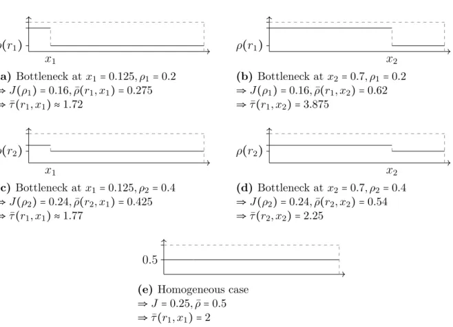
The really interesting feature of the travel time is shown in figure 3.6. The system with high jump rates all throughout the system in figure 3.6e is not the fastest, since it is in the maximum current phase where for every particle the probability to have its path blocked is equal to the average density of the system ρ =0.5. The fastest moving particles move through systems with a bottleneck right at the start in figure 3.6a, that prevents jamming all throughout the system. The lower current due to the bottleneck is overcompensated by the low density in the second part of the system.

(25)

3.6 Bottlenecks

x₁ ρ(r1)

(a) Bottleneck atx1=0.125, ρ1=0.2

⇒J(ρ₁) =0.16,ρ¯(r₁, x₁) =0.275

⇒τ¯(r₁, x₁) ≈1.72

x₂ ρ(r1)

(b) Bottleneck at x2=0.7, ρ1=0.2

⇒J(ρ₁) =0.16,ρ¯(r₁, x₂) =0.62

⇒τ¯(r₁, x₂) =3.875

x₁ ρ(r₂)

(c) Bottleneck at x1=0.125, ρ2=0.4

⇒J(ρ₂) =0.24,ρ¯(r₂, x₁) =0.425

⇒τ¯(r₁, x₁) ≈1.77

x₂ ρ(r₂)

(d) Bottleneck at x2=0.7, ρ2=0.4

⇒J(ρ₂) =0.24,ρ¯(r₂, x₂) =0.54

⇒τ¯(r₂, x₂) =2.25

0.5

(e) Homogeneous case

⇒J =0.25,ρ¯=0.5

⇒τ¯(r₁, x₁) =2

Figure 3.6.: Comparison of average density ¯ρ, currentJ and travel time ¯τ of four different bottleneck setups with bottleneck locationsx₁, x₂, densities after the bottleneckρ₁, ρ₂ (a)- (d) and the homogeneous case (e). The travel time is fastest in (a), because the small rate at the start of the system prevents jamming. The setup(c)is slower because the rate of the bottleneck is higher than in (a), causing a higher density after the bottleneck ρ and therefore increases the likelihood of jamming. If the bottlenecks are at the end of the system, the higher density setup (d)has a smaller travel time than (b).

The travel time is a function of both the location and the rate at the bottleneck. More details are discussed in the next section on the phase space of the travel time dependent on the defining parameters of the bottleneck, x and r.

3.6.2. Phase space of the travel time of a system with a bottleneck

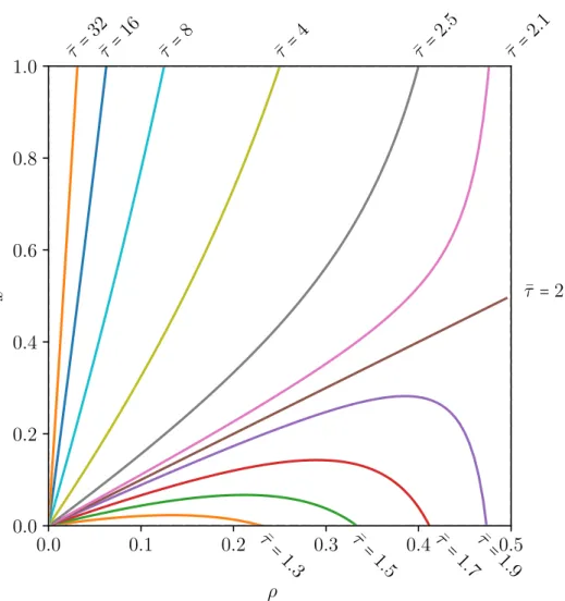
The right edge of the phase space in figure 3.7 is the homogeneous system (ρ=0.5). At this line, it is as if a rate r=1 were inserted into the system, leaving it homogeneous because there is in fact not bottleneck inside of the system. All but the travel time for the case where the lower current due to the insertion of a bottleneck is compensated by the lower average density (¯τ =2), never reach the line ρ=0.5. For any fixed ¯τ <2, the density and

(26)

3.6 Bottlenecks

location of the bottleneck only exist in a certain interval for both ρ and x¹. If ¯τ >2, the location of the bottleneck can be anywhere is the system, but there still is a maximum density if the bottleneck is at the end of the system.

In the case where the density ρ is fixed to a constant valueρc, the travel time is

¯ τ_c= 1

1−ρ_c +x( 1 ρ_c − 1

1−ρ_c) (3.14)

⇒¯τ_c∈ ( 1 1−ρ_c, 1

ρ_c). (3.15)

From the definition of the density ρ, it is known that

0<ρ_c<0.5 (3.16)

⇒1< 1

1−ρ_c <2 and 2< 1

ρ_c < ∞ (3.17)

and, depending on x, ¯τ_c can always assume values from an interval around the travel time of the homogeneous system, meaning that depending on x for any ρ_c the travel time can be smaller or larger than the travel time of the homogeneous system.

These results for the stationary TASEP with one bottleneck can be numerically verified for systems of lengthsL>100 and bottlenecks that are not too close to the initiation and termination regions to avoid edge effects. For the accuracy that I need for my statements later on, the distance has to be ≈10 sites away from the boundaries.

1The interval forxis given by

x∈

⎛

⎝ 0,1

2

⎛

⎝ 1−

√ τ¯ 2−τ¯

⎞

⎠

⎤

⎥

⎥⎥

⎥

⎦ .

The interval forρis given by

ρ∈ (0,1− 1

¯ τ] .

(27)

3.6 Bottlenecks

0.0 0.1 0.2 0.3 0.4 0.5

ρ 0.0

0.2 0.4 0.6 0.8 1.0

x ¯τ =2

¯ τ=32

¯ τ=16

¯ τ=8

¯ τ=4

¯ τ=2.5

¯ τ=2.1

¯ τ=1.3

¯ τ=1.5

¯ τ=1.7

¯ τ=1.9 ρ

Figure 3.7.: This figure shows the phase space of the travel time ¯τ. Each line represents a different value for the travel time ¯τ. The homogeneous case is the line ρ=0.5. The brown line, where ¯τ = 2 represents systems, where the lower current in the system is exactly compensated by the lower average density. All lines start from (0,0), but all but the line that compensates the current with the density approach the line ρ=0.5, but never reach it.The graphs were generated for different values of the travel time ¯τ by solving equation (3.13) for the relative location of the bottleneck x.

3.6.3. Interacting bottlenecks

When there are multiple bottlenecks present that are sufficiently far away from the boundaries and another, the strongest bottleneck, which is the one with the lowest rate, dominates the current J and density ¯ρ. The current J and density after the strongest bottleneck ρ are only dependent on the rate of this bottleneck, but not on the location. The average

(28)

3.6 Bottlenecks

density of the whole system ¯ρ is not only dependent on the rate, but also on the location x of the strongest bottleneck, cf. equation (3.13). This is visualized in figures 3.8 and 3.9.

(b) (a)

ωi

x₁ x₂

r₂ r₁

i

x₁ x₂

ρ_i

i 1−ρ(r₁)

ρ(r₁)

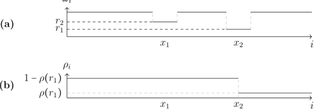
Figure 3.8.: An example system with two bottlenecks, r₁ and r₂. r₁ is at position x₁ and r2 atx2 withx1 <x2 and r1<r2. (a): The two bottlenecks in the system.r1<r2, therefore the density ρ in (b) is only dependent on r₁. The second bottleneck r₂ has no effects on the average density ¯ρ or the currentJ.

(b) (a)

ω_i

x₁ x₂

r₂ r₁

i

x₁ x₂

ρ_i

i 1−ρ(r1)

ρ(r₁)

Figure 3.9.: The example from figure 3.8, but with swapped rates. Because x₁ <x₂ and r₁ >r₂ in (a), the current is the same as before. But the average density changed and is now larger in (b). The first bottleneck r₁ has no effects on the average density ¯ρ or the current J.

Interacting bottlenecks are simple systems that can display sign epistasis (as described in section 2.4.1). This is easily visible when comparing the travel times ¯τ for all setups with two interacting bottlenecks in figure 3.6. In this example, the homogeneous wildtypeF₀ has the density ¯ρ=0.5, the currentJ=0.25 and the travel time per site ¯τ =2. Two synonymous mutations change the respective rates tor₁ and r₂ at positionsx₁ and x₂ span a landscape of 4 points with values of the measures from section 3.6.1.

(29)

3.6 Bottlenecks I explain in a later section 4.1, that there is no sign epistasis in the current J, because then the whole landscape is only dependent on the rates r₁, r₂, which are monotonic. If the measure chosen is the travel time, which is the average density divided by the current, the current is still monotonic in the rates, but the average density is not and therefore the travel time ¯τ is non-monotonic (cf. figure 3.6). Moreover, the travel time of interacting bottlenecks also shows neutral behavior. In figures 3.8 and 3.9, the larger bottleneck rate does not change the travel time of the system.

This interaction between the parameters is very interesting and is crucial for the model of interacting bottlenecks in chapter 5.

3.6.4. Relation between average density and bottleneck rate

There is no analytic function known for the relation between the average density ¯ρ and the bottleneck rate in the system r. But the relation between the two can be calculated numerically. The result of this comparison is figure 3.10. One can calculate the density ¯ρ of the TASEP with one bottleneck of rater and find the value for the density ρ, becauseρ is monotonic inr. This result can then be a map of densities to rates or rates to densities.

This monotonic behavior is the reason why the rate and the bottleneck density can be used interchangeably.

0.0 0.2 0.4 0.6 0.8 1.0

r 0.0

0.1 0.2 0.3 0.4 0.5

ρ

Figure 3.10.: The relation betweenρ and r is numerically approximated. The statistical noise at the end comes from the close proximity to the maximum current phase.

(30)

4. (Non-)Monotonic parameters in a TASEP with bottlenecks

In the following, results from literature and numerical results are compared. The goal is to find a parameter, that has the required attributes of the fitness landscape. As it is the most commonly used parameter to describe fitness in I start with the current as a potential candidate for a fitness measure. There is an example from literature that supposedly shows sign epistasis in the current from the paper by Fouladvand et al. [7]. I show the part of their results that supposedly shows sign epistasis in section 4.1. Afterwards I explain a new and unpublished analytic proof by Krug [17] that disagrees with the example from the literature. To support the statement from the proof I analyze the more general case of random systems in section 4.2 both with an analytic approximation by Szavits-Nossan et al. [28] and with a numerical simulation.

The last section 4.4 shows that the phase space of two interacting bottlenecks features the intersections between regions where the mutations exhibit sign epistatic interaction and regions where they do not change signs, which is postulated in section 4.3.

4.1. The current is monotonic in the jump rates

In their paper Fouladvand et al. describe a TASEP with rates drawn from a binary distribution [7]. This method constructs a system with a given percentile of the system being small rates and the other part equal to 1. Two figures from the paper show a current that increases, if slow rates are added into the system (cf. figures 4.1a, 4.2a). The system described in the paper has a fast initiation rate α=0.8 and slow termination rate β =0.05.

The other rates in the system are fast ω=1 with probability 1−f or have the rate ω=p1

with probability f. In figure 4.1a one can see an increase in the current, when comparing the homogeneous system at f =0 (so the system where all rates are equal to 1) to the inhomogeneous system at f=0.1 for all curves except forp₁ =0.05. The other homogeneous system atf =1 (here all rates are equal top₁) always has a smaller current than atf =0.9.

This would directly proof, that there is sign epistasis in the current, because increasing the amount of smaller rates has an opposite effect if the background is different. The opposite slopes are visible around f =0 andf =1. This is not in accordance with the intuition of a TASEP systems current, which should be monotonic in the amount of slow rates.

When trying to reproduce these results, I find exclusively monotonic behavior (cf. figures 4.1b,4.2b). The effect of changes on the particle current is always monotonic, meaning that an increase (decrease) of the jump rateω_i at any siteiin the system, causes the current to

(31)

4.1 The current is monotonic in the jump rates increase (decrease) or stay the same. I want to stress that this example is just one of the results presented in the paper and it is also described as "unexpected" in there and that the extreme cases (f =0,f =1) in both mine and their graphs are in accordance with the homogeneous TASEP for the ratesf =1 or f =p₁ respectively.

If one adapts part II A. from Krug [16] to the TASEP system, there can not be any sign epistasis in the current of the systems described by Fouladvand et al. [7]. Even though the proof is concerned with surface growth in condensed matter systems, the arguments can be applied here as well¹. Furthermore, this proof does not only hold for the quenched spatial disorder system from Fouladvand et al., but is also true for general TASEP systems.

(a)

0.0 0.2 0.4 0.6 0.8 1.0

f 0.02

0.03 0.04 0.05

J p1=0.05

p1=0.1 p1=0.3 p1=0.5

(b)

Figure 4.1.: Comparison between figure 8 from Fouladvand et al. [7] (a) and the same calculations with my own code (b). p₁ is the slower of two jump rates in the system.f is the percentile of sites that have rate p₁. J or <J > is the average current of the TASEP.

Both homogeneous cases, f =0 (all rates are 1) and f =1 (all rates are p₁) have the same values for J in both graphs but the behavior in the middle differs. In (a), the current is non-monotonic, in (b) the current is monotonic.

1This part is based on unpublished notes by Krug [17].

(32)

4.2 Small fully random systems analyzed with a power series approximation and numerical simulations

(a)

0.0 0.2 0.4 0.6 0.8 1.0

p1

0.00 0.02 0.04

J f=0.9

f=0.3 f=0.05 f=0.005

(b)

Figure 4.2.: Comparison between figure 14 from Fouladvand et al. [7] (a) and the same calculations with my own code (b). Here the parameter on the x-axis is the slower jump rate p₁. Like in figure 4.1, the curves from the paper show non-monotonic behavior while the curves simulated by my code do not.

With this result from my work and with the proof by Krug, I conclude that there can not exist any TASEP current that is non-monotonic in its rates.

4.2. Small fully random systems analyzed with a power series ap- proximation and numerical simulations

For systems with rates drawn from a distribution of random values, the current is a very complex function of the rates of the inhomogeneous TASEP. There is no general solution for it, but Szavits-Nossan et al. provide an analytical formula to compare to simulated data with their power series solution for the inhomogeneous TASEP with a small initiation rate α [28]. This is a result for a fully random system, with the constraint, that the initiation rate α is one order of magnitude smaller than the rest of the rates.

This is the analytic result, described by Szavitz-Nossan et al. [28] as the main result of their paper, for the expansion of the current J:

J(α) =α− 1

ω₁α²+ ( 1 ω₁ − 1

ω₂)⎛

⎝ 1 ω₂ +∑^L

j=3( 1

ω_j +δ_j,L 1 ω_L)∏^j

q=3

ωq

ω₁+ω_q

⎞

⎠α³+ O(α⁴) . (4.1) The epistasis measure described in equation (2.3) is used in the following analysis using a Mathematica code applying the equation (4.1). A small system size (L = 4) is filled with rates ω_i ∈ (0.1,1). The initiation rate is chosen from the interval α ∈ (0,0.1). The