Universität Konstanz Sommersemester 2015 Fachbereich Mathematik und Statistik

Universität Konstanz Sommersemester 2015 Fachbereich Mathematik und Statistik

Prof. Dr. Stefan Volkwein Sabrina Rogg

Optimierung

http://www.math.uni-konstanz.de/numerik/personen/rogg/de/teaching/

Program 2 (6 Points)

Submission by E-Mail: 2015/06/08, 10:00 h

Optimization with boundary constraints Implementation of the Gradient Projection Algorithm

So far we looked for (local) minimizer x ^∗ ∈ R ⁿ of a sufficiently smooth and real valued function f : R ⁿ → R in an open set Ω ⊆ R ⁿ :

x ^∗ = argmin

x∈Ω

f (x).

The first order necessary optimality condition is ∇f(x ^∗ ) = 0.

If Ω is given as the closed and bounded domain Ω =

n

Y

i=1

[a _i , b _i ] = {x ∈ R ⁿ | ∀i = 1, ..., n : a _i ≤ x _i ≤ b _i , a _i , b _i ∈ R , a _i < b _i },

the above condition must be changed to admit the possibility that a (local) minimizer is located on the boundary of the domain. In Exercise 11 we prove the following modified first order condition:

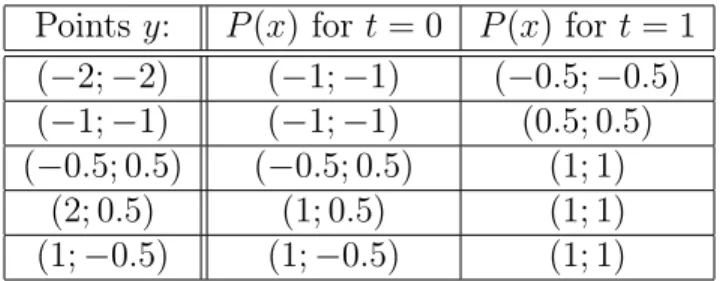
∇f (x ^∗ ) ^> (x − x ^∗ ) ≥ 0 for all x ∈ Ω. (1) The canonical projection of x ∈ R ⁿ on the closed set Ω is given by P : R ⁿ → Ω,

P (x)

i :=







a _i if x _i ≤ a _i x _i if x _i ∈ (a _i , b _i ) b _i if x _i ≥ b _i

.

It can be shown:

x ^∗ satisfies condition (1) ⇔ x ^∗ = P (x ^∗ − λ∇f (x ^∗ )) for all λ ≥ 0

The gradient projection algorithm (using the normalized gradient as descent direction) works as follows: Given a current iterate x ^k . Let d ^k := − _k∇f(x ^∇f(x

⁾

k

)k . The next iterate is set to

x ^k+1 = P (x ^k + t _k d ^k ), (2)

where t _k is a step length satisfying the following modified Armijo rule (compare Exercise 12):

f (x ^k+1 ) − f (x ^k ) ≤ −α

t _k kx ^k − x ^k+1 k ² . (3)

As termination criterion we use

kx ^k − P (x ^k − ∇f(x ^k ))k < . Part 1: Write a file projection.m for the function

function [px] = projection(x, a, b)

with the current point x ∈ R ⁿ , lower bound a ∈ R ⁿ and upper bound b ∈ R ⁿ as input arguments. The function returns the (pointwise) projected point px ∈ R ⁿ according to the canonical projection P . Note that this function can be implemented in one line.

Test your function for the rectangular 2-D domain defined by the lower bound (lower left corner) a = (−1; −1) ^> and the upper bound (upper right corner) b = (1; 1) ^> : compute the projection P (x) of points x = y + td ∈ R ² with y ∈ R ² as given in the table below, direction d = (1.5; 1.5) ^> ∈ R ² , step sizes t = 0 and t = 1. For validation compare your results to the projections given in the table:

Points y: P (x) for t = 0 P (x) for t = 1 (−2; −2) (−1; −1) (−0.5; −0.5) (−1; −1) (−1; −1) (0.5; 0.5) (−0.5; 0.5) (−0.5; 0.5) (1; 1)

(2; 0.5) (1; 0.5) (1; 1) (1; −0.5) (1; −0.5) (1; 1)

Table 1: Testing points and their projections with respect to t

Part 2: Write a function

function [t] = modarmijo(fhandle, x, d, t0, alpha, beta, amax, a, b) for the Armijo step size strategy with termination condition (3). The input arguments are as follows:

• fhandle: function handle

• x: current point

• d: descent direction

• t0: initial step size

• alpha, beta: parameters for the Armijo rule, the backtracking strategy

• amax : maximum number of iterations

• a, b: projection bounds

Part 3: Implement the gradient projection algorithm as described above. Generate a file gradproj.m for the function

function [X] = gradproj(fhandle, x0, epsilon, nmax, t0, alpha, beta, amax, a, b) with input parameters:

• fhandle: function handle

• x0: initial point

• epsilon: for the termination condition.

• nmax: maximum number of iteration steps

• alpha, beta, amax: parameters for the Armijo algorithm

• a, b: projection bounds

The program should return a matrix X = [x0, x1, x2, ...] containing the whole iter- ations.

Part 4: Call the function gradproj from a main file main.m to test your program for the Rosenbrock function

function [f,g] = rosenbrock(x)

with input argument x ∈ R ² and output arguments the corresponding function value f

∈ R and gradient g ∈ R ² . Use the parameters epsilon=1.0e-2, nmax=1.5e+3, t0=1, alpha=1.0e-2, beta=0.5, amax = 30. Take the following initial values and bounds:

1. x0=[1;-0.5], a=[-1;-1] and b=[2;2]

2. x0=[-1;-0.5], a=[-2;-2] and b=[2;0]

3. x0=[-2;2], a=[-2;-2] and b=[2;2]

Visualize the results in suitable plots and write your observations in the written report.