Regional Growth in Central Europe:
Long-term Effects of Population and Traffic Structure
Wolfgang Polasek
Helmut Berrer
Regional Growth in Central Europe: Long-term Effects of Population and Traffic Structure
ISSN: Unspecified
2005 Institut für Höhere Studien - Institute for Advanced Studies (IHS) Josefstädter Straße 39, A-1080 Wien
E-Mail: o ce@ihs.ac.atffi Web: ww w .ihs.ac. a t
All IHS Working Papers are available online: http://irihs. ihs. ac.at/view/ihs_series/
This paper is available for download without charge at:
https://irihs.ihs.ac.at/id/eprint/1645/
Regional Growth in Central Europe
Long-term Effects of Population and Traffic Structure
Wolfgang Polasek and Helmut Berrer
Regional Growth in Central Europe
Long-term Effects of Population and Traffic Structure
Wolfgang Polasek and Helmut Berrer July 2005
Institut für Höhere Studien (IHS), Wien
Institute for Advanced Studies, Vienna
Contact:
Wolfgang Polasek
Department of Economics and Finance Institute for Advanced Studies Stumpergasse 56
1060 Vienna, Austria : +43/1/599 91-155 email: polasek@ihs.ac.at
Helmut Berrer
Department of Economics and Finance Institute for Advanced Studies Stumpergasse 56
1060 Vienna, Austria : +43/1/599 91-112 email: berrer@ihs.ac.at
Founded in 1963 by two prominent Austrians living in exile – the sociologist Paul F. Lazarsfeld and the economist Oskar Morgenstern – with the financial support from the Ford Foundation, the Austrian Federal Ministry of Education and the City of Vienna, the Institute for Advanced Studies (IHS) is the first institution for postgraduate education and research in economics and the social sciences in Austria.
The Economics Series presents research done at the Department of Economics and Finance and aims to share “work in progress” in a timely way before formal publication. As usual, authors bear full responsibility for the content of their contributions.
Das Institut für Höhere Studien (IHS) wurde im Jahr 1963 von zwei prominenten Exilösterreichern – dem Soziologen Paul F. Lazarsfeld und dem Ökonomen Oskar Morgenstern – mit Hilfe der Ford- Stiftung, des Österreichischen Bundesministeriums für Unterricht und der Stadt Wien gegründet und ist somit die erste nachuniversitäre Lehr- und Forschungsstätte für die Sozial- und Wirtschafts- wissenschaften in Österreich. Die Reihe Ökonomie bietet Einblick in die Forschungsarbeit der Abteilung für Ökonomie und Finanzwirtschaft und verfolgt das Ziel, abteilungsinterne Diskussionsbeiträge einer breiteren fachinternen Öffentlichkeit zugänglich zu machen. Die inhaltliche Verantwortung für die veröffentlichten Beiträge liegt bei den Autoren und Autorinnen.
Europe is explored as how they depend on the young and old dependency ratio. The young dependency ratio (YDR) is defined as ratio of the less than 20 years old and the old dependency ratio (ODR) as the more than 60 years old divided by the total population. We found a medium sized negative correlation of these ratios on regional growth and the long- term forecasts for the year 2020 are for most regions rather negative if only the population structure is considered. Similar scenarios can be also obtained for employment and population growth. The long-term forecasts improve if traffic accessibilities and dynamic interactions are introduced into the model.
Keywords
Panel data, Simpson paradox, GDP, employment and population growth, long-term forecasts
JEL Classification
R1, R41, L92, C21
1. Introduction 1 2. GDP growth and population structure 3
2.1 Long Term Forecast Implications ... 4 2.2 Long Term Forecasts and Traffic Infrastructure (TI)... 8 2.3 Long Term Forecasts and Dynamic Structure (DS) ... 10
3. Employment growth and population structure 13
3.1 Long-term forecast implications for employment growth ... 15 3.2 Long Term Forecasts and Traffic Infrastructure (TI)... 17 3.3 Long Term Forecasts and Dynamic Structure (DS) ... 18
4. Population growth and population structure 20
4.1 Long Term Forecast Implications ... 22 4.2 Long Term Forecasts and Traffic Infrastructure (TI)... 24 4.3 Long Term Forecasts and Dynamic Structure (DS) ... 26
5. A CART Analysis 28
6. Conclusions 30
References 31
1. Introduction
Age structure and growth have become a highly disputed topic for growth scenarios of countries around the world. Some papers have explored the impact of the age structure on economic growth (see e.g. Brunow and Hirte 2005). But only a few econometric results are available on a regional level with panel data. This short note explores the effect of regional growth in six European countries for the period 1995 to 2001: Austria, Hungary, Slovakia, Poland, Germany and the Czech Republic.
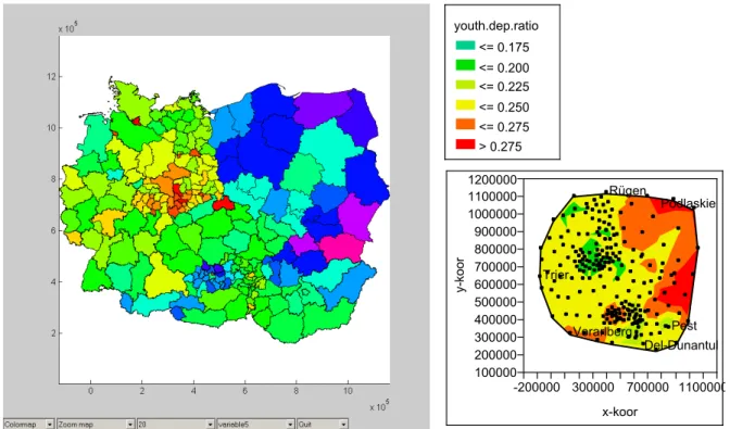
Figure 1.1 shows the young dependency ratio (YDR) over the 227 regions and we see a large dependency ratio along the eastern border of Poland and Slovakia. But surprisingly, also some smaller cells of upper Austria, East Tyrol, Vorarlberg and Salzburg have a dependency ratio of above 25%. The contour plot is based on the coordinates of the region centres and interpolates the YDR variable. Small values of the young dependency ratio can be seen for irregularly shaped regions in Saxony and a small stretch near the Netherlands border.
Figure 1.2 shows the old dependency ratio and clearly the cells in eastern Germany,
especially in Saxony, exhibit the largest old dependency ratio, but also in Western Germany
most cells show high values. In Austria we see the northern regions of lower Austria,
Burgenland and Upper Styria to have high old dependency ratios. The regions in Northwest
Poland have the lowest ODR ratios of six the countries. While Poland can be divided into
four regions if we look at the map of the old dependency ratios, many of the regions in the
Czech Republic and Hungary have also “old dependency” of about 20%.
youth.dep.ratio
<= 0.175
<= 0.200
<= 0.225
<= 0.250
<= 0.275
> 0.275
100000 200000 300000 400000 500000 600000 700000 800000 900000 1000000 1100000 1200000
y-koor
Vorarlberg Pest Del-Dunantul Rügen
Trier
Podlaskie
-200000 300000 700000 1100000 x-koor
Figure 1.1: Young dependency ratio YDR: (0-20 years / Pop.) and contour plot
old.dep.ratio
<= 0.175
<= 0.188
<= 0.200
<= 0.213
<= 0.225
<= 0.238
<= 0.250
<= 0.263
> 0.263
100000 200000 300000 400000 500000 600000 700000 800000 900000 1000000 1100000 1200000
y-koor
Vorarlberg Pest Del-Dunantul Rügen
Trier
Podlaskie
-200000 300000 700000 1100000 x-koor
Figure 1.2: Old dependency ratio ODR: (60+ / Pop.) and contour plot
2. GDP growth and population structure
In the following section we explore the relationship between regional GDP growth and the young and old dependency ratios.
Table 2.1: Correlation matrix of GDP growth and the dependency ratios YDR and ODR (p-values in parenthesis)
(p-val) GDP% YDR ODR
GDP% 1 0.39 -0.41
YDR (0.0) 1 -0.82
ODR (0.0) (0.0) 1
Note: all correlations are significantly different from zero.
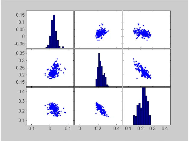
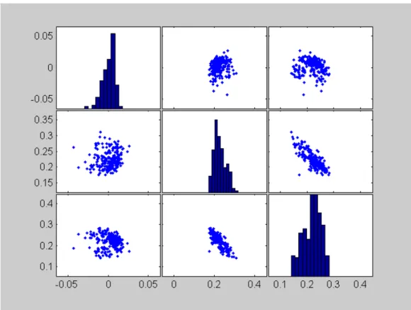
Figure 2.1: Scatterplot-matrix of GDP growth and the dependency ratios YDR and ODR
From Figure 2.1 and the correlation table 2.1 we see that the correlation coefficient between
GDP growth and the young dependency ratio is positive while the correlation coefficient
between GDP growth and the old dependency ratio is negative. As a consequence both
dependency ratios (ODR and YDR) are negatively correlated. This can be also seen from the
scatter plot matrix that summarizes the 227 regions in central Europe.
2.1 Long Term Forecast Implications
For the year 2020 long-term population growth projections are available from the statistical offices in the six countries. From these forecasts for 2020 we computed the future young and old dependency ratio and used them for a conditional forecast for the GDP growth in the year 2020. In order to compare the impact of the population structure on GDP growth we also computed the difference between the past estimates and the estimated forecasts.
First, in Table 2.2, we computed the simple regression models to explore the effects of old and young dependency ratios on the GDP growth rate, and in table 2.3 we computed the fixed effect regression model, i.e. we substituted the intercept by the six dummy variables for the six countries.
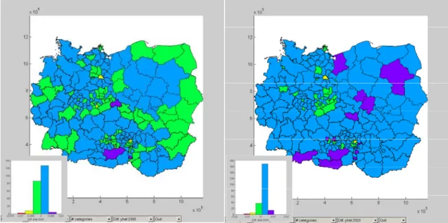
In Figure 2.3 we plotted a map of the fitted values of the fixed effect models for 2000 and in Figure 2.4 the forecasts of the fixed effect model for the regressor data of 2020. These fitted values are the point forecast for GDP growth for the year 2020, given the (official) forecasts of young and old dependency ratios for 2020, but the coefficients of the model are based on the data observation from 1995 to 2001.
Table 2.2: Regression estimates for the simple model
OLS coeff. Conf-Intervals.
b b_lower b_upper
intercept 0.030 -0.017 0.076 young DR 0.096 -0.025 0.218
old DR -0.130 -0.230 -0.031
R2 F-Stat p-value
0.175 23.68 0
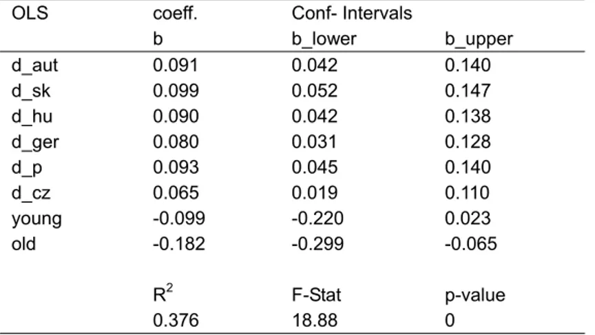
Table 2.3: Regression estimates for the fixed effect model and population structure (PS)
OLS coeff. Conf- Intervalsb b_lower b_upper d_aut 0.091 0.042 0.140 d_sk 0.099 0.052 0.147
d_hu 0.090 0.042 0.138
d_ger 0.080 0.031 0.128 d_p 0.093 0.045 0.140
d_cz 0.065 0.019 0.110
young -0.099 -0.220 0.023 old -0.182 -0.299 -0.065
R2 F-Stat p-value
0.376 18.88 0
For interpretation purposes we refer to the measurement scale of dependency ratios, i.e. the values from 0 to 1 as percentages or 100 basis points (bp). From the simple model we see that the increase of 10 basis points in the YDR increase the GDP growth by about 1%-point.
The effect of 10 bp of the ODR is negative and larger: about -1.2%-points. Note that in the fixed effect model both effects are negative and ODR coefficient is double the size. 10bp difference in the DR will decrease GDP growth of about 1%-point for YDR and -1.8%-points for ODR. If there were no old or young people in the population we see from the fixed effects that average growth could lie between 6.5% pa (CZ) and 9.9% (SK):
Figure 2.2: Scattergrams of GDP% with YDR and ODR: Simpson paradox visualized
The regression estimates in Table 2.2 and Table 2.3 show that the so-called Simpson effect is present in the data. While in the simple regression model the coefficient of the young dependency ratio is positive, it is negative for the fixed effect model. This means if we condition the regression of GDP growth on the six countries, we observed a negative correlation between growth and young dependency ratio, while for the simple model we see a positive slope, implying that the growth rates of the six countries were rather widely and heterogeneously distributed.
Note that Simpson Paradox can best explain the reversal of the sign of the YDR coefficient.
The youth dependency ratios are increasing with faster growing countries, as can be seen
from Figure 2.2, while the connection of GDP growth and YDR within countries is mainly
negative. This negative slope can be estimated if we control for the within country
relationships by the fixed effects.
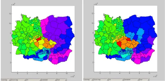
Figure 2.3: Estimated GDP% (yhat) for 2000 Figure 2.4: Forecasted GDP% for 2020
Figure 2.5: Difference of forecasts (yhat 2020 - yhat 2000) due to population structure
Note that these country dummies double the size of the R
2; nevertheless the overall strength of the relationship is small and it is of no surprise if this effect on population structure cannot be found in complex (dynamic) regression models of GDP growth.
Figure 2.3 shows that the lowest GDP growth is estimated by the fixed effect (and PS) model for the Czech regions. This is because the Czech Republic experienced two recession years (1997 and 1998), which leads to a depressed average growth rate. The highest GDP% rates can be found in Hungary, notable the Budapest corridor and the regions along the Polish western border. The second highest growth rates are found in PL and SK, and in Austria along the “Westbahn” (Vienna-Bregenz) corridor.
Figure 2.4 maps the predictions from the fixed effect model for the year 2020. The highest regional growth rates can be seen for HU, the second highest for PL, SK and Austria. CZ comes last.
The difference of fitted values (yhat 2020 - yhat 2000) in Figure 2.5 shows that the values for
all regions are negative, which is due to increasing dependency ratios. We see that the
maximum negative effect on yearly GDP growth is observed for northern Bohemia. Also
around Sczeczin and Wroclaw (Silesia in Poland) the regions suffer from the predicted Old
dependency ratio in 2020. Note that whole of Germany (including Eastern Germany),
Hungary and Slovakia will only be slightly affected, but all regions in the Czech Republic will
have a growth disadvantage. Similar growth impediment can be seen for most regions in
Poland, except for the eastern border regions. Surprisingly the alpine regions in Austria
except East Tyrol will loose growth potentials due to adverse population structure, which
should be explored in more detail.
2.2 Long Term Forecasts and Traffic Infrastructure (TI)
In the following we add to the model traffic infrastructure variables.
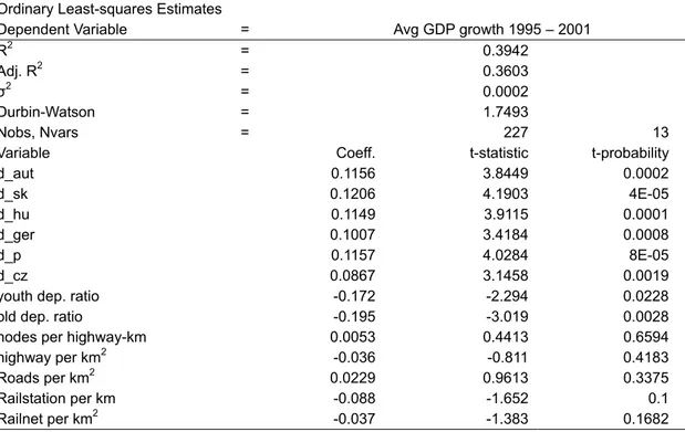
Table 2.4: Regression estimates for population structure (PS) and traffic infrastructure (TI)
Ordinary Least-squares Estimates
Dependent Variable = Avg GDP growth 1995 – 2001
R2 = 0.3942
Adj. R2 = 0.3603
σ2 = 0.0002
Durbin-Watson = 1.7493
Nobs, Nvars = 227 13
Variable Coeff. t-statistic t-probability
d_aut 0.1156 3.8449 0.0002
d_sk 0.1206 4.1903 4E-05
d_hu 0.1149 3.9115 0.0001
d_ger 0.1007 3.4184 0.0008
d_p 0.1157 4.0284 8E-05
d_cz 0.0867 3.1458 0.0019
youth dep. ratio -0.172 -2.294 0.0228 old dep. ratio -0.195 -3.019 0.0028 nodes per highway-km 0.0053 0.4413 0.6594
highway per km2 -0.036 -0.811 0.4183 Roads per km2 0.0229 0.9613 0.3375 Railstation per km -0.088 -1.652 0.1
Railnet per km2 -0.037 -1.383 0.1682 Legend:
nodes per highway-km : Number of highway entrances per highway-km highway per km2: Autobahn Km per region-area
Roads per km2: Total Road length per region-area
Railstation per km: Number of railway stations per railway-net km Railnet per km2: railway-net per region-area
From Figure 2.6a we see the differences of fitted GDP% rates between the fixed effect model and the traffic infrastructure (TI) augmented regression model. Traffic induced growth is generally scattered around city regions while the strongest positive differences have been observed for structural weak regions in Northern CZ (Liberec), Upper Styria and south Burgenland (both AT).
Figure 2.6b shows the difference of growth forecasts for the year 2020. Again, the best
forecasts can be seen for regions in Poland and Austria while only a few regions will not
benefit: These are some Polish regions (including Warsaw) and Alpine regions in Austria.
Figure 2.6a: Difference of average growth esti- mates (yhat 2000(PS&TI) – yhat 2000 (PS) ) due to traffic infrastructure
Figure 2.6b: Difference of growth forecasts (yhat 2020(PS&TI) – yhat 2020(PS) ) due to traffic infrastructure
2.3 Long Term Forecasts and Dynamic Structure (DS)
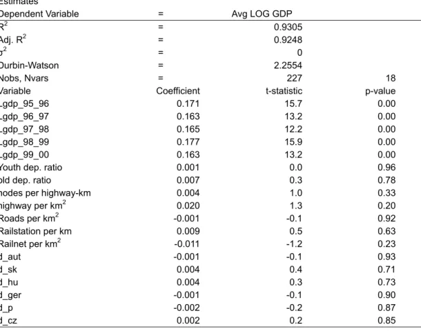
Table 2.5: Regression estimates for population structure (PS), traffic infrastructure (TI) and time dynamics (DYN)
Ordinary Least-squares Estimates
Dependent Variable = Avg LOG GDP
R2 = 0.9305
Adj. R2 = 0.9248
σ2 = 0
Durbin-Watson = 2.2554
Nobs, Nvars = 227 18
Variable Coefficient t-statistic p-value
Lgdp_95_96 0.171 15.7 0.00
Lgdp_96_97 0.163 13.2 0.00
Lgdp_97_98 0.165 12.2 0.00
Lgdp_98_99 0.177 15.9 0.00
Lgdp_99_00 0.163 13.2 0.00
Youth dep. ratio 0.001 0.0 0.96 old dep. ratio 0.007 0.3 0.78 nodes per highway-km 0.004 1.0 0.33
highway per km2 0.020 1.3 0.20 Roads per km2 -0.001 -0.1 0.92 Railstation per km 0.009 0.5 0.63
Railnet per km2 -0.011 -1.2 0.23
d_aut -0.001 -0.1 0.93
d_sk 0.004 0.4 0.71
d_hu 0.004 0.3 0.73
d_ger -0.001 -0.1 0.90
d_p -0.002 -0.2 0.87
d_cz 0.002 0.2 0.85
Figure 2.7a: Difference of fitted average growth ( yhat 2000( PS & TI & DYN ) – yhat 2000( PS & TI) ) due to time dynamics
Figure 2.7b: Difference of growth forecasts ( yhat 2020( PS & TI & DYN ) –
yhat 2020( PS & TI ) ) due to time dynamics
Figure 2.7a and Figure 2.7b shows the differences of fitted GDP% rates between the traffic infrastructure regression model and the time dynamic augmented model. Interestingly, the dynamic effects are scattered around the whole six countries. For example, Budapest and Warsaw will profit from a dynamic development if it is similar as in the past. This shows that the dynamic component in the model is rather regional heterogeneous.
Table 2.6: R
2Increase by model nesting for GDP %
R2 Diff. R2
PS 0.1745 6D (country dummies) 0.3487 0.17
6D + PS (population structure) 0.3763 0.03 6D + PS + TI (Traffic
infrastructure)
0.3942 0.02 6D + PS + TI + Dynamics (lagged
dep. variables)
0.9269 0.53
Comparing the R
2of nested models in Table 2.6 yield the following insights: 17% of the R
2is explained by the dummy variables. Population structure and traffic infrastructure is also week, between 2 and 3%. Only the time domain explains more than ½ for the model fit: 53%.
R2 BMA Diff. R2
PS 0.1745 6D (country dummies) 0.3487 0.17
6D + PS (population structure) 0.3763 0.03 6D + PS + TI (Traffic infrastructure) 0.3942 0.02 6D + PS + TI + Dynamics (lagged
dep. variables) 0.9269 0.53
3. Employment growth and population structure
In the following section we explore the relationship between regional employment growth and the young and old dependency ratios.
Table 3.1: Correlation matrix of EMPL growth and dependency ratios (p-values in parenthesis)
(p-val) EMPL% YDR ODR EMPL% 1.00 0.13 0.08 YDR (0.049) 1.00 -0.82 ODR (0.24) (0.0) 1.00
Figure 3.1: Scatterplot-matrix of employment growth and the dependency ratios YDR and ODR
From Figure 3.1 and the correlation Table 3.1 we see that the correlation coefficient between
employment growth and the young dependency ratio is positive (and significant) while the
correlation coefficient between GDP growth and the old dependency ratio is not significantly
positive.
Table 3.2: Regression estimates for the simple employment model
OLS coeff. Conf-Int.
b b_lower b_upper
intercept -0.024 -0.059 0.012 young DR 0.082 -0.011 0.174
old DR 0.029 -0.047 0.104
R2 F-Stat p-value
0.0195 2.2265 0.1103
Table 3.3: Regression estimates for the fixed effect model
OLS coeff. Conf-Int.
b b_lower b_upper
d_aut 0.0539 0.019 0.0887 d_sk 0.0516 0.018 0.0853
d_hu 0.0252 -0.0089 0.0594
d_ger 0.0478 0.0134 0.0823 d_p 0.0321 -0.0015 0.0656
d_cz 0.0315 -0.0006 0.0636
young -0.0192 -0.1054 0.067 old -0.1859 -0.2686 -0.1032
R2 F-Stat p-value
0.3604 17.6278 0
From the simple regression model we see that the R
2is very low and both regression
coefficients have a positive sign. Again by the looking at the fixed effect model, we see that
the R
2is about he same size as for the GDP growth model and both coefficients are
estimated negatively. The YDR coefficient is not significant while the ODR coefficient has the
same size as in the GDP growth model. For the employment model it is possible that the
negative relationship might not reflect a direct economic connection, rather we suspect it is
the indirect connection via GDP growth.
Figure 3.2: Scattergrams of employment growth with YDR and ODR
3.1 Long-term forecast implications for employment growth
In the simple model we estimated the annual employment growth based on youth and old dependency ratios (and the fixed effects) and we calculated the fit 2000 and the forecasts 2020. As before, we compute the difference between the fitted values for 2000 and the forecasted values for 2020.
Figure 3.3:
Estimated EMPL% values (yhat) for 2000
Figure 3.4: Forecasted EMPL% values (yhat) for 2020
Figure 3.5: Differences (of yhat) between 2020 and 2000
From Figure 3.3 we see that the simple model explains (i.e. the effects of the population structure) high employment growth rates in Austria and Hungary, zero employment growth effects for most German regions, while only some shrinking employment growth effects for Slovakia and Czech Republic.
Figure 3.4 predicts for the year 2020 by the simple model positive employment growth effects for almost all regions in Hungary and Austria (except upper Styria and the northern lower Austria). German regions are very mixed: some stay with zero employment growth effects, but several other regions can improve, like e.g. in Bavaria, Baden-Würtenberg, Frankfurt and the regions around Berlin. Surprisingly we find on the loser side most of the regions in the Czech Republic and Poland, where surprisingly the regions west of Warsaw are negatively affected but the regions at the eastern border are not.
Figure 3.5 shows the difference of the employment growth rates due to the influence of the
population structure. Through all the regions we see a negative EMPL% contribution. The
highest reductions are expected for western Poland and the lowest growth losses for
Hungary. Germany and Hungary are less affected by the population structure than Austria
and SK.
3.2 Long Term Forecasts and Traffic Infrastructure (TI)
Table 3.4: Regression estimates for EMPL structure (PS) and traffic infrastructure (TI)
Ordinary Least- squares Estimates
Dependent Variable = Avg LOG EMPL growth 1995-2001
R2 = 0.3952
Adj. R2 = 0.3613
σ2 = 0.0001
Durbin-Watson = 1.9476 Nobs, Nvar = 227 13
************************************************************************************************************
Variable Coefficient t-statistic p-value youth dep. ratio -0.018 -0.3 0.73
old dep. ratio -0.172 -3.8 0.00 nodes per highway-km 0.009 1.1 0.27 highway per km2 0.048 1.6 0.12 Roads per km2 -0.034 -2.1 0.04 Railstation per km 0.038 1.0 0.30 Railnet per km2 0.000 0.0 0.98
d_aut 0.051 2.4 0.02
d_sk 0.049 2.4 0.02
d_hu -0.018 -0.3 0.73
d_ger -0.172 -3.8 0.00
d_p 0.009 1.1 0.27
d_cz 0.048 1.6 0.12
Figure 3.6a:
Difference of average EMPL%fits (yhat 2000(PS&TI) – yhat 2000(PS) ) due to Traffic Infrastructure.
Figure 3.6b:
Difference of average EMPL%forecasts (yhat 2020(PS&TrInf) – yhat 2020(PS) ) due to Traffic infrastructure.
Figure 3.6a shows that the difference of EMPL% rates due to traffic variables is around 0 for most of the regions but positive for western German regions along the Rhine valley. Also some regions in Austria will benefit, while some regions in Eastern Germany were not affected by traffic infrastructure. The forecast of these differences for the year 2020 in Figure 3.6b is less favourable since more regions are 0 or slightly small positive.
3.3 Long Term Forecasts and Dynamic Structure (DS)
The next Table 3.5 shows the regression estimates for the full model, i.e. using Population structure, Traffic infrastructure and dynamic components:
Table 3.5: Regression estimates for EMPL structure (PS), traffic infrastructure (TI) and time dynamics (DYN)
Ordinary Least-squares Estimates Dependent Variable = = Avg LOG EMPL growth 1995 – 2001
R2 = 0.8615
Adj. R2 = 0.8502
σ2 = 0
Durbin-Watson = 1.4932
Nobs, =227, Nvar 18
****************************************************************************************************
Variable Coefficient t-statistic p-value Lempl_95_96 0.120 11.9 0.00 Lempl_96_97 0.161 13.3 0.00 Lempl_97_98 0.184 14.0 0.00
Lempl_98_99 0.117 6.4 0.00
Lempl_99_00 0.194 12.1 0.00 youth dep. ratio -0.046 -1.8 0.07
old dep. ratio -0.050 -2.2 0.03 nodes per highway-km 0.005 1.2 0.24
highway per km2 0.019 1.2 0.22 Roads per km2 -0.011 -1.3 0.18 Railstation per km 0.027 1.5 0.13
Railnet per km2 -0.007 -0.7 0.47
d_aut 0.023 2.2 0.03
d_sk 0.022 2.2 0.03
d_hu 0.021 2.1 0.04
d_ger 0.020 2.0 0.05
d_p 0.018 1.9 0.06
d_cz 0.020 2.1 0.03
Figure 3.7b: Difference of EMPL% forecasts (yhat 2020(PS&TI&Dyn) – yhat 2000(PS&TI) ) due to time dynamics Figure 3.7a: Difference of EMPL% fit (yhat 2000
( PS & TI & Dyn) – yhat 2000( PS &
TI )) due to time dynamics
Figure 3.7a shows the difference of EMPL% rates with respect to time dynamics. We see that only a few cells in Eastern Germany and southern Poland were negatively affected. In the long run for 2020 we see that dynamic time effects are only large for the western and central regions in Poland. Employment growth does not respond heavily to short-term time dynamic effects for most of the other regions
Table 3.6: R
2Increase by model nesting EMPL%
R2 Diff. R2
PS 0.0195 0
6D (country dummies) 0.2737 0.25 6D + PS (population structure) 0.3604 0.09 6D + PS + TI (Traffic infrastructure) 0.3952 0.03 6D + PS + TI + Dyn (lagged dep.
variables)
0.8615 0.47
From Table 3.6 we see that the country dummy variables explain 25% of the R
2, the
population structure 9% and the traffic infrastructure 3%. The largest amount, 47% is due to
the dynamic component.
4. Population growth and population structure
Table 4.1: Correlation matrix of population growth and the dependency ratios YDR and ODR (p-values in parenthesis)
(p-val) GDP% YDR ODR GDP% 1.00 0.26 -0.23 YDR (0.0) 1.00 -0.82 ODR (0.0) (0.0) 1.00
First we notice from Table 4.1 and Figure 4.1 that population growth is positively correlated with the YDR and negatively with the ODR.
Figure 4.1: Scatterplot-matrix of population growth and the dependency ratios
YDR and ODR
Table 4.2: Regression estimates for the simple population model
OLS coeff. Conf-Int.
b b_lower b_upper
intercept -0.0123 -0.0373 0.0128 young DR 0.0639 -0.0009 0.1287
old DR -0.0126 -0.0658 0.0406
R2 F-Stat p-value
0.0684 8.2254 0.0004
Table 4.3: Regression estimates for the fixed effect model
OLS coeff. Conf-Int.
b b_lower b_upper
d_aut 0.012 -0.0167 0.0407 d_sk 0.0098 -0.0179 0.0375
d_hu 0.0016 -0.0266 0.0297
d_ger 0.0125 -0.0158 0.0409 d_p 0.0016 -0.026 0.0292
d_cz 0.0063 -0.0202 0.0327
young 0.0563 -0.0147 0.1273 old -0.1079 -0.1761 -0.0398
R2 F-Stat p-value
0.1619 6.0434 0
The simple regression model has a very poor fit (R
2= 6.8%) but the F-statistic is significant
and the sign of the regression coefficients follow the signs of the bivariate correlations of the
correlation matrix. In the fixed effect model the sign pattern is confirmed and the negative
effect of the ODR is more pronounced. A 10 bp increase in the ODR will reduce on average
the population growth by 1.1%-point while a 10 bp increase in the YDR will stimulate the
population growth by 0.6%-point. Note that even if the size of the old and young population
group would be equal the net effect would be negative on the population growth.
Figure 4.2: Scattergrams of GDP% with YDR and ODR
4.1 Long Term Forecast Implications
As before, we explore the forecast behaviour of the model with respect to the population growth. In Figure 4.3 and 4.4 we have estimated annual population growth based on youth and old dependency ratios for the years 2000 and 2020.
Figure 4.3: Estimated Pop% values (yhat) for 2000
Figure 4.4: Forecasted POP% values (yhat) for 2020
Figure 4.5: Differences (of yhat) between 2020 and 2000
From Figure 4.4 we see that the model for population growth fits a bimodal distribution,
where most of the German regions belong to the low growth group of about 1.8% and many
of the Austrian regions, together with a band of regions stretching from Slovakia along the
eastern border of Poland belong to the high growth group of 3%. The picture of the
population growth rate distributions again bimodal if we look at the model forecasts of 2020
in Figure 4.5. The forecasts for most of the German regions are just below 1% and for the
Polish and Slovak regions it is between 2% and 3%. If we look at Figure 4.5 to see where the
main losers of the population growth forecasts due to a shifting population structure are, we
see that Germany, Slovakia and Hungary are reducing the growth rate marginally, while in
the central band the regions from the Alps to the Baltic Sea the reduction of the population
growth rate is on average about 1%. Also we see that the forecast of the population growth
follows roughly the pattern of the forecasts of the employment growth rates.
4.2 Long Term Forecasts and Traffic Infrastructure (TI)
Table 4.3: Regression estimates for population structure (PS) and traffic infrastructure (TI)
Ordinary Least-squares Estimates
Dependent Variable = Avg LOG POP growth 1995 – 2001
R2 = 0.2039
Adj. R2 = 0.1593
σ2 = 0.0001
Durbin-Watson = 1.7656
Nobs, =227 Nvars = 13
*********************************************************************************************************
Variable Coefficient t-statistic p-value youth dep. ratio 0.034 0.8 0.43
old dep. ratio -0.099 -2.7 0.01 nodes per highway-km 0.008 1.2 0.23
highway per km2 0.025 1.0 0.32 Roads per km2 -0.014 -1.0 0.31 Railstation per km -0.010 -0.3 0.75
Railnet per km2 -0.014 -0.9 0.37
d_aut 0.017 1.0 0.32
d_sk 0.014 0.9 0.40
d_hu 0.034 0.8 0.43
d_ger -0.099 -2.7 0.01
d_p 0.008 1.2 0.23
d_cz 0.025 1.0 0.32
Figure 4.6b: Difference of population forecasts (yhat 2020(PS&TI) – yhat 2020(PS) ) due to Traffic Infrastructure
Figure 4.6a: Difference of average
population fit (yhat 2020(PS&TI) – yhat 2000(PS) ) due to Traffic Infrastructure
In Figure 4.6a we see the difference of the average population fit due to traffic infrastructure.
We see that the positive growth differences for 2000 are in the majority and surprisingly more population growth was observed in western region than in the east. The forecast for 2020 in Figure 4.6b shows a different picture: All Polish regions are profiting from traffic impulses, the Alpine regions in Austria and Western German regions. Only a few regions will get negative impulses.
In Figure 4.7a we see that for the estimates in the model time dynamics was not contributing
to population growth. Only the ring of regions around Berlin was profiting from a new
dynamic at the end of the 90ies. Other Eastern German regions lost due to the dynamic
component, as well as regions in Moravia and southern Austria. The forecast for 2020 can
be seen in Figure 4.7b: Zero growth differences are only expected in a few regions, most of
the in Eastern German. Most regions are getting positive impulses from time dynamics.
4.3 Long Term Forecasts and Dynamic Structure (DS)
Table 4.3: Regression estimates for population structure (PS), traffic infrastructure (TI) and time dynamics (DYN)
Ordinary Least-squares Estimates
Dependent Variable = Avg LOG POP growth 1995 - 2001
R2 = 0.911
Adj. R2 = 0.9037
σ2 = 0
Durbin-Watson = 2.0796
Nobs, Nvars = 227, 18
Variable Coefficient t-statistic p-value
Lpop_95_96 0.055 0.8 0.41
Lpop_96_97 0.151 3.3 0.00
Lpop_97_98 0.282 6.0 0.00
Lpop_98_99 0.237 3.7 0.00
Lpop_99_00 0.370 8.8 0.00
youth dep. ratio 0.000 0.0 0.98 old dep. ratio -0.002 -0.1 0.90 nodes per highway-km 0.003 1.4 0.18
highway per km2 -0.009 -1.0 0.33 Roads per km2 0.004 0.7 0.45 Railstation per km -0.002 -0.2 0.86
Railnet per km2 -0.001 -0.2 0.86
d_aut 0.000 0.0 0.98
d_sk 0.006 1.0 0.33
d_hu -0.001 -0.1 0.90
d_ger 0.000 0.0 0.98
d_p -0.002 -0.3 0.73
d_cz 0.001 0.2 0.86
Figure 4.7b: Difference of POP% forecasts (yhat 2020(PS&TI&Dyn) – yhat
2020(PS&TI) ) due to time dynamics Figure 4.7a: Difference of average population fit
(yhat 2000(PS&TI&Dyn) – yhat 2000(PS&TI) ) due to time dynamics
Table 4.7: R
2Increase by model nesting for POP%
PS R2 Diff. R2
6D (country dummies) 0.0405
6D + PS (population structure) 0.1619 0.12 6D + PS + TI (Traffic infrastructure) 0.2039 0.04 6D + PS + TI + Dyn (lagged dep. variables) 0.911 0.71
Table 4.7 shows that 71% of the R
2measure can be explained by the past population
dynamics. The traffic infrastructure component is weak; the population structure contributes
3 times as much to the model fit, namely 12%.
5. A CART Analysis
In Figure 5.1 we estimated a classification and regression tree (CART) model for the GDP growth rate model. We see that the first variable to build a tree is the splitting of the distribution by the variable YDR. The R
2of the model is 0.365.
If YDR is less than 24% the regional GDP growth decreases to 1.9% otherwise it increases to 3.3% (this was the case for about ¼ of the regions. If in the low GDP growth group the ODR is above 20% then the GDP growth declines to 1.5%, otherwise it increases slightly to 2.2%. In the upper branch we see that the fastest growing regions were those, where the number of rail stations was low (but these were only six cells). But “on top” to this phenomenon we see that the regional GDP growth can be boosted if the ODR is less than 10%: Growth goes up to 3.5%.
In Figure 5.2 we estimated a classification and regression tree (CART) model for the employment growth rate (EMPL). We see that the first variable to define a tree is the splitting of the distribution by the variable GDP per employee (GDP_pw). The R
2of the model is 0.335.
We see that for regions with a high GDP per employee the EMPL growth rate is 6.0% while
for low GDP per employee the EMPL growth rate is –1%. This shrinking EMPL growth rate
can only be turned into a positive growth rate of the YDR is larger than 27%. Then the EMPL
growth rate is 5.8%, but only 16 regions fulfil this condition. Otherwise we see that the EMPL
growth rate drops further, down to –4.3%, and this trend in only reversed at the –1% level if
the old ODR is less than 25%. (These have been 98 regions in the period 1995-2001.)
Count Mean Std Dev
227 0.0226762 0.0158338
All Rows
Count Mean Std Dev
162 0.0186356 0.0145778
YDR<0.24
Count Mean Std Dev
79 0.0148741 0.012395
ODR>=0.2
Count Mean Std Dev
83 0.0222158 0.0156366
ODR<0.2
Count Mean Std Dev
6 0.0029014 0.0079401
ODR<0.1
Count Mean Std Dev
77 0.0237208 0.0150968
ODR>=0.1
Count Mean Std Dev
65 0.0327466 0.0143661
YDR>=0.24
Count Mean Std Dev
59 0.0297074
0.010032
RSt/km>=0.005
Count Mean Std Dev
38 0.0266996 0.0100672
ODR>=0.1
Count Mean Std Dev
21 0.03515 0.007488
ODR<0.1
Count Mean Std Dev
6 0.0626322
0.017133
RSt/km<0.005
Figure 5.1: Partitioned CART model for GDP growth
Count Mean Std Dev
227 0.0142247 0.0689832
All Rows
Count Mean Std Dev
150 -0.00946 0.0668715
Lgdp_pw<3.77
Count Mean Std Dev
134 -0.017455 0.0619848
YDR<0.27
Count Mean Std Dev
36 -0.042972 0.0610875
ODR>=0.25
Count Mean Std Dev
98 -0.008082 0.0599262
ODR<0.25
Count Mean Std Dev
16 0.0575 0.0707069
YDR>=0.27
Count Mean Std Dev
77 0.0603636 0.0460411
Lgdp_pw>=3.77
Figure 5.2: Partitioned CART model for EMPL %
6. Conclusions
The simple forecasting exercise has shown that the regional GDP growth rates will suffer heavily from the age structure, i.e. the dependency ratios in the year 2020. If no other factors will dominate GDP growth in future, the regional growth rate which was observed until 2001 in central Europe will be not sustainable in the future.
The size of the effects varies across countries: While GDP growth in Germany, Hungary and Slovakia will be almost not affected by a changing population structure, most regions in Poland, Austria and the Czech Republic will suffer from adverse population structure effects.
Interestingly, the employment rate depends only significantly negatively from the ODR, while the population growth depends positively on the ODR and YDR. The forecast scenarios for 2020 show very different pattern in the six central European countries of regional growth according to the three variables GDP, employment and population growth.
The main findings of the study are:
1) All six central European countries suffer growth losses due to an aging population structure until 2020. This aging population stress will affect annual growth in some regions up to 2% points per year.
2) This adverse age effect is offset by favourable stimuli stemming from improved infrastructure investment, like railways or roads. Traffic infrastructure will benefit in first line big centre (or metropolitan) regions and such effects will spill over in the surrounding regions (neighbourhood effects: this has been seen very clearly for the 5 regions around Berlin.) On average, the adverse population aging effect will be offset by the positive affect of infrastructure on growth.
3) Many important influences on regional growth could not be measured and therefore we see a large dynamic component dominating the long-term forecasting behaviour. Since the dynamic component could only be observed for a short period it is unclear if this observed trend will last until the year 2020. Important effect like the migration component was not part of the regional model, since it was impossible to get reliable yearly data for all the cells in the six central European countries.
4) In summary regional GDP growth in central European regions will be rather constant in
the next one or two decades. Only in some regions we will observe a dynamic process,
which will have rather specific regional reasons. Thus there will be room for many
regional success stories, but no simple overall recipe can be concluded from the
dynamic panel model. Thus regional growth, which will be larger than the current basic
zero growth outlook, will be based on very heterogeneous dynamic regional
components.
References
Barro, R. and Sala-I-Martin X. (1992), "Convergence," Journal of Political Economy, No. 100, pp. 223-251.
Barro, R. and Sala-I-Martin X. (1995), Economic Growth, McGraw Hill: New York.
Brunow, St. and Hirte G. (2005) “Age structure and Regional Income Growth,” TU Dresden, Discussion paper Verkehr 1/2005.
LeSage, J. P. (1997), “Bayesian Estimation of Spatial Autoregressive Models,” International
Regional Science Review, 1997 Volume 20, 113-129.LeSage, J. P. (1999a), “A Family of Geographically Weighted Regression Models,” Paper presented at the Regional Science Association International meetings, Santa Fe, NM.
LeSage, J. P. (1999b), “Geographically Weighted VAR models,” mimeo, University of Toledo.
http://www.spatial-econometrics.com
Moore, D. S. and G. P. McCabe (2003), Introduction to the Practice of Statistics, Fourth Edition, WH Freeman & Co.
Polasek, W. and H. Berrer (2005a), “Spatio-Temporal GDP forecasts for Central European Regions,” IHS Vienna, mimeo.
Polasek, W. and H. Berrer (2005b), “Infrastructure and GDP growth in Central European Regions,” IHS Vienna, mimeo.
Raftery, A., D. Madigan, and J.A. Hoeting (1997), “Bayesian Modeling Averaging for Linear
Regression Models,” Journal of the American Statistical Association 92, 179-191.
Authors: Wolfgang Polasek and Helmut Berrer
Title: Regional Growth in Central Europe: Long-term Effects of Population and Traffic Structure Reihe Ökonomie / Economics Series 172
Editor: Robert M. Kunst (Econometrics)
Associate Editors: Walter Fisher (Macroeconomics), Klaus Ritzberger (Microeconomics) ISSN: 1605-7996
© 2005 by the Department of Economics and Finance, Institute for Advanced Studies (IHS),
Stumpergasse 56, A-1060 Vienna • +43 1 59991-0 • Fax +43 1 59991-555 • http://www.ihs.ac.at