Adaptive Forecasting of the EURIBOR Swap Term Structure

SFB 649 Discussion Paper 2008-017

Adaptive Forecasting of the EURIBOR Swap

Term Structure

Oliver Blaskowitz*

Helmut Herwartz**

* Humboldt-Universität zu Berlin, Germany

** Christian-Albrechts-Universität zu Kiel, Germany

This research was supported by the Deutsche

Forschungsgemeinschaft through the SFB 649 "Economic Risk".

http://sfb649.wiwi.hu-berlin.de ISSN 1860-5664

SFB 649, Humboldt-Universität zu Berlin

S FB

6 4 9

E C O N O M I C

R I S K

B E R L I N

Adaptive Forecasting of the EURIBOR Swap Term Structure.

^∗

Oliver Blaskowitz

Humboldt–Universit¨at zu Berlin Institute of Statistics and Econometrics

Phone: +49 – 30 – 2093 – 5705 Email: blaskowitz@wiwi.hu–berlin.de

Helmut Herwartz

Christian–Albrechts–Universit¨at zu Kiel Institute of Statistics and Econometrics

Phone: +49 – 431 – 880 – 2417 Email: herwartz@stat–econ.uni–kiel.de Abstract

In this paper we adopt a principal components analysis (PCA) to reduce the dimensionality of the term structure and employ autoregressive models (AR) to forecast principal components which, in turn, are used to forecast swap rates. Arguing in favor of structural variation, we propose data driven, adaptive model selection strategies based on the PCA/AR model. To evaluate ex-ante fore- casting performance for particular rates, different forecast features such as mean squared errors, directional accuracy and big hit ability are considered. It turns out that relative to benchmark models, the adaptive approach offers additional forecast accuracy in terms of directional accuracy and big hit ability.

Keywords: Principal components, ex–ante forecasting, EURIBOR swap rates, term struc- ture, directional accuracy, big hit ability.

JEL classification: C32, C53, E43, G29.

∗This research was supported by the Deutsche Forschungsgemeinschaft through the SFB 649 ‘Economic

Risk’.

1 Introduction

While term structure modelling has undergone extensive improvements, advances in term structure forecasting are comparatively small. Yet, the latter is particularly important for purposes of managing risk or hedging derivatives. Diebold & Li (2006) point out that the empirical performance of model based out–of–sample forecasts is rather poor. Reformulating the Nelson & Siegel (1987) model, they use autoregressive models for the factors to obtain encouraging results for long horizon ex–ante forecasts. While Diebold & Li (2006) find that forecasts based on vector autoregressive models (VARs) outperform forecasts implied by the random walk model, Duffee (2002) concludes that the random walk model is superior to standard affine term structure models.

Ang & Piazzesi (2003) model yield curves by means of traditional latent yield factors and observable macroeconomic variables. Forecast error variance decompositions show that macro factors explain up to 85% of the variation in bond yields. Taking a dynamic factor approach Diebold, Rudebusch & Aruoba (2006) model the yield curve by means of latent level, slope and curvature factors as well as macroeconomic variables as real activity, inflation and the federal funds rate. They find convincing evidence of the macroeconomic effects on the yield curve. M¨onch (2007) forecasts the yield curve in a data rich environment. He uses a factor–augmented VAR jointly with an affine term structure model with parameter restrictions implied by a no–arbitrage condition. The model turns out to outperform different benchmark models such as a random walk, standard VAR and the Diebold & Li (2006) approach among others.

Though a large part of the term structure literature is concerned with factor models, a uniform conclusion with regard to the appropriate number of factors has not been achieved yet. Nelson & Siegel (1987) introduce a parsimonious three factor model for term structures and conclude that it is able to capture important yield curve characteristics. Numerous extensions of the Nelson–Siegel model exist. Inter alia, a two factor version is applied by Diebold, Piazzesi and Rudebusch (2005) and the four factor version from Svennson (1994) is frequently used by central banks (BIS 2005). Empirical support is provided by Litterman

& Scheinkman (1991) and Steeley (1990). Their factor, respectively, principal component analysis (PCA) suggests that most of the term structure variation can be explained by three factors, interpreted as level, slope and curvature. Examining money market returns, Knez,

Litterman & Scheinkman (1994) present a four factor model to find that the additional factor is related to private issuer credit spreads. Duffie & Singleton (1997) advocate a multi factor model for interest rate swaps that accommodates counterparty default risk and liquidity differences between Treasury and Swap markets. They conclude that credit and liquidity factors are important sources to explain swap term structure dynamics. Within this framework Liu, Longstaff & Mandell (2006) estimate a five factor model to analyze swap spreads.

To explain forecast failures of macroeconomic models, Clements & Hendry (2002), among others, argue that economies evolve and are subject to changes, e. g., in institutions or technology. Neglecting the change of economic relations is a potential reason for the poor performance of model based out–of–sample term structure forecasts. To admit for dynamic heterogeneity, data based adaptive forecasting procedures appear to be useful alternatives.

Swanson and White (1997a,b) find that an adaptive approach yields promising results in forecasting macroeconomic variables. A particular issue in dynamic ex–ante forecasting is the stability of model parameters. Splitting a sample of US government interest rates covering the period January 1970 to December 1995 into three parts, Bliss (1997) concludes that factor loadings varied only slightly. Yet, factor volatilities turned out to be relatively stable. For US zero coupon bond yields Audrino, Barone–Adesi & Mira (2005) find that loadings are unstable over the period from January 1986 to May 1995 in a three factor model allowing for conditional heteroscedasticity.

A large fraction of the term structure literature is concerned with the US treasury market.

However, Remolona & Wooldridge (2003) point out that the EURO swap market has become one of the largest and most liquid markets world wide. The enormous increase in hedging and positioning activity tripled the turnover in Euro denominated interest rate swaps between 2000 and 2006 (ECB 2007).

Due to the huge size of swap markets and the neglected attention paid to forecasting the term structure, we focus on forecasting the EURIBOR (European interbank offered rate) swap term structure. Employing a purely statistical factor model approach, we decompose the term structure of swap rates by means of PCA and apply AR models to compute (adap- tive) forecasts. Using various combinations of the number of factors, AR orders and time windows, our analysis includes a set of 100 model specifications. The latter are evaluated in

terms of mean squared forecast errors, directional accuracy and big hit ability.

Similar to H¨ardle, Herwartz & Spokoiny (2003) we argue in favor of dynamic variation of the term structure and motivate an adaptive procedure relying on local homogeneity of the term structure. By means of several data driven model selection algorithms, we analyze the relative performance of an adaptive approach and particular ‘unconditional’ PCA/AR forecasting schemes. Compared with standard benchmark models an adaptive approach offers additional forecast accuracy in terms of directional accuracy and big hit ability.

The remainder of the paper is organized as follows. The factor model approach is pre- sented in the next Section. In Section 3 we introduce the loss measures used to evaluate forecasting performance. Sections 4 and 5 describe the data and characterize the uncondi- tional approach to motivate adaptive model selection procedures. Section 6 proposes partic- ular adaptive strategies. Moreover, we compare the adaptive strategies to unconditionally implemented factor models as well as to some benchmark models. Section 7 concludes.

2 A forecast model for the swap rate term structure

The investigated EURIBOR swap term structure consists of daily swap rates for M = 10 maturities (3 months (3m), 6m, 1 year, 2years (2yr), 3yr, 5yr, 7yr, 10yr, 12yr and 15yr). Let

˜

y_t= (˜y_1,t,y˜_2,t, . . . ,y˜_M,t)⁰ denote the 10 dimensional vector of observed swap rates measured in terms of deviations from their unconditional mean, ˜y_t =y_t−y¯_T^∗, y¯_T^∗ = 1/τPT^∗

t=T^∗−τ+1y_t. To generate rolling swap rate forecasts we summarize the dynamic variation of the term structure in a time window of size τ by a few underlying factors. More precisely, equations (2.1) and (2.2) below constitute the local description of the term structure

˜

yt = ΓKFt+ξt, t=T^∗−τ+ 1, . . . , T^∗, (2.1)

∆Ft = ν+ Φ1∆Ft−1+. . .+ Φp∆Ft−p+ηt . (2.2) In (2.1) theK–dimensional vectorFtconsists of factorsfk,tthat govern the term structure. In (2.2) the first differences for eachf_k,t, k = 1, . . . , K, are assumed to follow ’cross sectionally’

uncorrelated AR(p) processes. Hence, Φ1, . . . ,Φp are diagonal matrices and ηt is a K–

dimensional zero mean error term with a diagonal covariance matrix. Moreover, the error terms ξt and ηt are assumed to be ’cross sectionally’ and serially uncorrelated. The matrix Γ_K in (2.1) is obtained by means of PCA which decomposes the unconditional covariance

matrix of ˜yt, i.e.

Σˆ_T^∗ = 1 τ

T^∗

X

t=T^∗−τ+1

˜

y_ty˜_t⁰, Σˆ_T^∗ = ΓΛΓ⁰. (2.3) In (2.3) the eigenvectors of ˆΣ_T^∗ constitute the matrix Γ and the diagonal matrix Λ contains the corresponding eigenvalues in decreasing order. To account for the variation explained by the K most important principal components, the matrix Γ_K consists of the first K columns of Γ. Note that even if PCA and factor analysis are conceptually different, they are closely related (see e.g. Johnson & Wichern 2002). Thus, we do not distinguish between factors and principal components.

To implement ex–ante forecasting of swap rates the K most important factors F_t = (f_1t, . . . , f_Kt)⁰ are estimated asFb_t = Γ⁰_Ky˜_t for t=T^∗−τ+ 1, . . . , T^∗.First differences of the factors are modelled by univariate AR(p) processes

∆fb_k,t =γ_k0 +γ_k1∆fbk,t−1+. . .+γ_kp∆fbk,t−p+u_k,t, k = 1, . . . , K.

Iterated h–step forecasts for the first differences, ∆fb_k,T^∗_+h|T^∗, are computed as

∆fb_k,T^∗+h|T^∗ =bγ_k0+bγ_k1∆fb_k,T^∗+h−1|T^∗+. . .+bγ_kp∆fb_k,T^∗+h−p|T^∗,

where bγ_k0, . . . ,bγ_kp are OLS estimates of γ_k0, . . . , γ_kp and ∆fb_k,T^∗+j|T^∗ = ∆fb_k,T^∗_+j if j ≤ 0.

Then, factor ‘level’ forecasts are

fb_k,T^∗+h|T^∗ =fb_k,T^∗+

h

X

j=1

∆fb_k,T^∗+j|T^∗.

Finally, theh–step ahead forecast of the swap rate term structure conditional on information available at time T^∗ is

yb_T^∗+h|T^∗ = Γ_KFb_T^∗+h|T^∗+ ¯y_T^∗, where ¯y_T^∗ readjusts for the unconditional in–sample mean.

Note that we compute principal components from centered swap rate levels. If swap rates are non stationary then some eigenvectors of Γ may be interpreted as (unidentified) cointegration parameters (Johansen 1995), and PCA yields at least some non stationary factors. For our forecasting procedures it turns out that results for AR models specified in first differences of the factorsF_tare more stable than for AR models in levels. Finally, in the

local model the drift parameterν in (2.2) implies a linear trend in the levels of interest rates.

While such a feature contradicts theoretical and empirical long run interest rate properties, in the presence of local trends, however, including the parameter ν might be beneficial for ex–ante forecasting procedures.

To generate h–step forecasts for a particular swap rate m in time T^∗ by means of the local model given in (2.1) and (2.2) an analyst has to choose the parameters τ, K and p. In this study, we consider a set of 100 competing model specifications implied by combining a variety of choices for τ, K, p. Then, an adaptive model selection approach is based on out–

of–sample forecast performance evaluated with particular loss functions such as quadratic loss, directional accuracy and big hit ability.

3 Loss functions

Before motivating the loss functions considered in this study, we briefly introduce some nota- tion. Let a general loss function depend on theh–step ahead swap rate forecast, ˆy_m,T^∗+h|T^∗, the current swap rate,y_m,T^∗ and the future (true, realized) swap rate,y_m,T^∗_+h,with maturity m, i.e.

L^h,m_T∗ =L(ˆy_m,T^∗+h|T^∗, y_m,T^∗, y_m,T^∗_+h). A common loss function is the quadratic loss:

L^h,m_1,T∗ = (y_m,T^∗_+h−yˆ_m,T^∗+h|T^∗)². (3.1) Diebold & Mariano (1995) point out that in light of the variety of economic decision problems relying on forecasts, statistical loss functions such as the quadratic loss do not necessarily conform to economic loss functions. In an interest rate setting, Swanson &

White (1995) show that the mean squared forecast error (MSFE) and profit measures are not closely linked. Similarly, Leitch & Tanner (1991) find that, opposite to MSFE, the directional accuracy (DA) of forecasts, i. e. the ability of correctly predicting directions, is highly correlated with profits in a term structure analysis. Lai (1990) points out that an investor can still gain profits even with statistically biased forecasts if they are characterized by significant DA. Ash, Smith & Heravi (1998) indicate that qualitative statements on the change of the economy in the near future are important pre–requisites for the appropriate implementation of monetary and fiscal policy. Similarly, ¨Oller & Barot (2000) emphasize the

importance of DA for central banks as a forecast of increased inflation (above target) would prompt central banks to raise interest rates. WithI(•) denoting an indicator function a loss function for DA is:

L^h,m_2,T∗ = I (ˆy_m,T^∗+h|T^∗−y_m,T^∗)(y_m,T^∗+h|T^∗ −y_m,T^∗)>0

−I (ˆy_m,T^∗+h|T^∗−y_m,T^∗)(y_m,T^∗+h|T^∗ −y_m,T^∗)<0 .

Hatzmark (1991) investigates forecast ability by looking at DA and ‘Big Hit Ability’. To motivate the latter, it might occur that a profit seeking trader is better able to predict big price changes rather than small changes. In this case, forecast performance could depend on a small number of correct directional forecasts generating large profits, and a large number of incorrect directional forecasts associated with negligibly small losses. A loss function for Big Hit Ability (BH) is:

L^h,m_3,T∗ =L^h,m_2,T∗|y_m,T^∗_+h−y_m,T^∗|

The BH measure generalizes the quadratic loss and DA statistics in that it takes the sign as well as the magnitude of the movement into account. If y_m,T^∗ is a swap rate, L^h,m_3,T∗ is only approximately a profit function. The profit/loss from closing a swap position in T^∗ +h is given by the swap value in T^∗ +h since in T^∗ a swap with a (fair value) fixed rate y_m,T^∗ has a value of zero. However, as a swap is a financial derivative, in T^∗ +h the value of a swap with rate y_m,T^∗ is a non linear function of y_m,T^∗_+h (Miron & Swannell 1991). Yet, as the second derivative of the swap value function with respect to y_m,T^∗_+h, is often very small, most traders and risk managers consider swaps as linear instruments even if they are actually non linear. That is to say upward/downward movements iny_m,T^∗_+h are almost proportional to changes in the profit/losses from closing the corresponding swap position.

4 Data

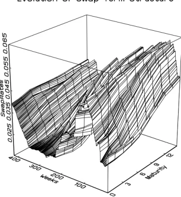
We investigate closing rates for Eurozone interest rate swaps with maturity 1yr, 2yr, 3yr, 5yr, 7yr, 10yr, 12yr and 15yr and the 3m resp. 6m Euribor rate as obtained from the database EcoWin (http://www.ecowin.com/). The sample period comprises 2100 daily observations (Mon through Fri) from February 15, 1999, to March 2, 2007. Figure 1 shows the evolution of the swap term structure. It displays the variability of the term structure shape over time. For example, the level of the swap term structure is higher in October/November

2000 (around week 100) than in March 2004 (around week 280). Similarly, the slope of the term structure is higher in March 2003 (around week 210) as e. g. in November 2007 (around week 400). Moreover, the curvature in November 2003 (around week 250) exceeds the corresponding measure in October 2001 (around week 140).

Table 1 documents that all observed term structures increase with a minimum slope measure of 0.01. Consequently, the average term structure is also increasing. Swap rates at long maturities exhibit less variation than those at the short end. For the curvature the evidence is mixed. The sample mean (median) of this quantity indicates a slightly concave curvature of -0.00543 (-0.00325) with minimum and maximum values between - 0.0825 and 0.084, respectively. Hence, on average the curvature of the term structure is not very pronounced, although Figure 1 uncovers locally concave/convex patterns.

5 Unconditional forecast models

We consider 4 forecast horizons (h = 1,5,10,15 days) and focus on h–step forecasts of 2yr, 5yr and 10yr swap rates. Hence, overall there are 12 distinct forecast ‘exercises’ F E_j = {m^j, h^j}, j = 1, . . . ,12, where F E_j is a tuple from the cartesian set defined by {2,4,8} × {1,5,10,15}. To define the adaptive strategies let a particular model specification be denoted byM_s ={τ^s, K^s, p^s}, where

τ^s ∈ Ω_τ ={42,63,126,189,252} , K^s ∈ Ω_K ={1,2,3,4,5} ,

p^s ∈ Ω_p ={0,1,2,3}.

Ms is a three dimensional tuple from the cartesian set Ωτ × ΩK ×Ωp the cardinality of which is 100. A forecast for a specification s at time T^∗ is ˆy_m,T^s ∗+h|T^∗. For a particular loss function L^h,m,s_i , i = 1,2,3, and each model specification Ms an average out–of–sample forecast performance over the time interval [T₁^∗;T₂^∗] is

1 T₂^∗−T₁^∗+ 1

T₂^∗

X

T^∗=T₁^∗

L^h,m,s_i,T∗ = 1 T₂^∗−T₁^∗+ 1

T₂^∗

X

T^∗=T₁^∗

L_i(ˆy_m,T^{s ∗}_+h|T^∗, y_m,T^∗, y_m,T^∗_+h).

We refer to the average loss associated with L^h,m,s_i , i= 1,2,3, respectively, as MSFE, mean directional accuracy (MDA) and mean big hit ability (MBH). The average losses of model

specification s in forecasting rate m at horizon h are denoted by MSFE^h,m_s , MDA^h,m_s and MBH^h,m_s .

To motivate an adaptive model selection approach we first consider the ‘unconditional’

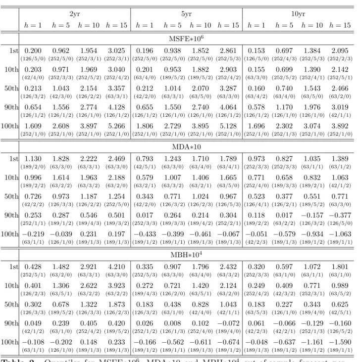
forecast performance, i. e. the average forecast performance of the 100 models M_s for the period T₁^∗ = 308 (April 19, 2000) to T₂^∗ = 2085 (February 9, 2007). Table 2 shows the MSFEs obtained when forecasting the 2yr swap rate one day ahead (h= 1). The best model is approximately 8 times better than the worst model, the 10th best model is still more than 3 times better than the 90th best model. For MDA and MBH the overall picture is similar.

Hence, choosing the wrong model may provide poor forecasts. Moreover, for MDA and MBH the latter conclusion holds throughout for all forecast exercises F E_j. For the MSFE criterion, however, the ‘spread’ between the best and worst models diminishes for forecast horizons h >5.

[Insert Table 2 about here]

In addition to marked differences in relative model performance, forecasting accuracy of a particular factor model might vary over time. In case of structural variation each factor model specification might be seen as an approximation of the true data generating process and the approximation accuracy of particular models depends on ‘local’ term structures.

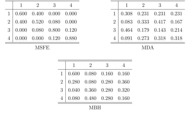
To describe time varying model performance we consider transition probability matrices as in Camba–Mendez, Kapetanios & Weale (2002). Each of the 100 models is mapped to performance quartiles conditional on the first and second half of the sample period. The transition probabilities are obtained from counting the models that move from one quartile in the first to a particular quartile in the second subsample. While a diagonal transition matrix indicates performance stability, large off–diagonal entries hint at performance instability.

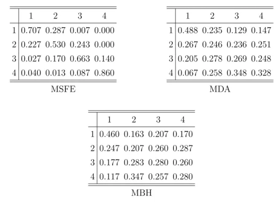
Table 3 shows the transition probabilities for the accuracy measures MSFE, MDA and MBH for the 2yr rate and h = 1. The upper left panel of Table 3 refers to the MSFE criterion.

While there are transitions within the two upper and the two lower quartiles, there are not so many transitions crossing the subsample medians. The respective patterns for the MDA and MBH measures are remarkably different, and indicate much more transitions across quartiles. Off–diagonal elements take values between 0.083 and 0.417, respectively, 0.04 and 0.48. Again, the results are similar over all horizonsh= 1,5,10,15 and swap rates 2yr, 5yr, 10yr (see the average transition matrices in Table 8 given in the appendix). For a similar data

set, Blaskowitz, Herwartz & de Cadenas (2005) conclude that model parameters τ, K and p do not have a uniform impact on the forecasting performance. In summary, we diagnose marked heterogeneity of model specifications in terms of MDA and MBH performance while with respect to model implied MSFE measures model choice appears less crucial.

[Insert Table 3 about here]

In light of time dependent forecast accuracy it is desirable to have a strategy at hand that ex-ante identifies the locally best model. In the next Section we describe and evaluate data driven model selection strategies.

6 Adaptive strategies

6.1 Data driven model selection

An unconditional model approach is inherently subjected to misspecification under changing relations between economic variables. The rolling window strategy allows the parameters of a model to evolve over time. Yet, if parameter values are exposed to variation one may conjecture that the quality of a model approximation is time specific as well. An adaptive selection/estimation strategy is a promising means to account for distinct relative forecasting performance.

Our data adaptive model selection approach is based on a further time window of eτ = 42 days in which the ‘local’ out–of–sample performance of specifications M_s, s= 1, . . . ,100, is evaluated. Choosing evaluation windows of length τe = 42 is thought to balance between the needs of modeling flexibility under local heterogeneity on the one hand and statistical precision of parameter estimates on the other hand.

At each time point T^∗ the most recent eτ h−step forecast errors for swap rate m and model specification Ms are known. A local MSFE measure is

MSFE^h,m,s_T∗ =

T^∗−h

X

t=T^∗−h−eτ+1

L^h,m,s_1,t /τ .e

The adaptive strategy, denoted MinMSFE, chooses the local MSFE minimizing specification:

ˆ

y_m,T^MinMSFE∗+h|T^∗ = ˆy_m,T^s∗ ∗+h|T^∗, s^∗ = argmin

s=1,...,100

{MSFE^h,m,s_T∗ } .

Another strategy to adaptively select a particular model specification is based on an ANOVA regression of the local MSFEs of the 100 factor models M_s on dummy variables representing the model parameters τ, K and p. The AnoMSFE forecast is given by

ˆ

y_m,T^AnoMSFE∗+h|T^∗ = ˆy^s_m,T^∗ ∗+h|T^∗ ,

where s^∗ ={τ^∗, K^∗, p^∗} is the locally best model specification as indicated by the smallest estimated (dummy variable) coefficients for τ, K and p (see also Blaskowitz, Herwartz and de Cadenas 2005).

Among others, Diebold & Pauly (1987) argue that in the presence of structural shifts composite forecasts can improve forecast precision. Numerous combining procedures have been proposed in the literature. We focus on both an equal weight scheme and a combination procedure that assigns different weights to individual forecasts. The Av10MSFE forecast is

ˆ

y^Av10MSFE_m,T∗+h|T^∗ = 1 10

ˆ

y_m,T^s∗1 ∗+h|T^∗+. . .+ ˆy_m,T^s∗10 ∗+h|T^∗

,

where M_s^∗

1, . . . , M_s^∗

10 refer to the 10 best models in terms of MSFE^h,m,s_T∗ . Conditional on M_s^∗

1, . . . , M_s^∗

10 the BunnMSFE forecast is given by ˆ

y_m,T^BunnMSFE∗+h|T^∗ = ˆθ_s^∗

1yˆ_m,T^s∗1 ∗+h|T^∗ +. . .+ ˆθ_s^∗

10yˆ^s_m,T^∗10 ∗+h|T^∗ ,

where the weights ˆθ_s^∗_q, q = 1, ...,10,are proportional to the number of times (out ofτeforecast realizations) that model s^∗_q outperforms all other 9 models in terms of smaller squared error (Bunn 1975).

Along similar lines as described for the MSFE criterion we also use the loss functions MDA and MBH for adaptive forecasting.

Finally, we employ two combining strategies that have found support in the empirical literature (Clemen 1989). The AvStrat resp. MedStrat take the average resp. median forecast of the 100 forecast models irrespective of past performance. At time T^∗ these forecasts are given by

ˆ

y^AvStrat_m,T^∗_+h|T^∗ = 1 100

100

X

s=1

ˆ

y_m,T^{s ∗}_+h|T^∗, ˆ

y^MedStrat_m,T^∗_+h|T^∗ = Median

s=1,...,100

yˆ^s_m,T^∗_+h|T^∗ .

In summary, the set of adaptive strategies is

Ω_AS = {MinMSFE, Av10MSFE, AnoMSFE, BunnMSFE, MaxMDA, Av10MDA, AnoMDA, BunnMDA, MaxMBH, Av10MBH, AnoMBH, BunnMBH, AvStrat, MedStrat}.

All forecast comparisons are performed over the same sample period comprising 1778 time instances. Hence, accounting for the largest estimation window (τ = 252), the highest forecast horizon (h = 15) and the model evaluation window (eτ = 42), the rolling forecasting analysis starts in time point T₁^∗ = 252 + 15 + 42−1 = 308. Average losses of a particular adaptive strategy AS and forecast exercise F E_j are denoted by MSFE^h,m_AS , MDA^h,m_AS and MBH^h,m_AS . To compare the performance of the adaptive strategies we provide respective normalized average losses. Normalization is accomplished with respect to the best and worst unconditional models in terms of average loss:

nMSFE^h,m_AS = 1−

MSFE^h,m_AS −min

s

MSFE^h,m_s maxs

MSFE^h,m_s −min

s

MSFE^h,m_s ,

nMDA^h,m_AS =

MDA^h,m_AS −min

s

MDA^h,m_s maxs

MDA^h,m_s −min

s

MDA^h,m_s ,

nMBH^h,m_AS =

MBH^h,m_AS −min

s

MBH^h,m_s maxs

MBH^h,m_s −min

s

MBH^h,m_s .

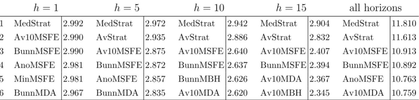
For a given forecast horizon the sum of normalized losses for forecasts of the 2yr, 5yr and 10yr rates for the six best strategies are provided in Table 4. For the MSFE criterion it can be seen that the MedStrat strategy produces for all horizons superior normalized losses.

The AvStrat strategy performs slightly worse for horizons h = 5,10,15 and is overall the 2nd best performing strategy. The Av10MSFE strategy is for all horizons among the best 3 adaptive strategies. In terms of MDA and MBH the MedStrat is again overall the best strategy. For h = 1,10,15 normalized losses are always better than the normalized losses of at least all but one adaptive strategy. In contrast to the MSFE criterion the Av10MDA resp. BunnMDA strategies are overall the second resp. third best competitor strategies.

6.2 Unconditional models vs. adaptive strategies

Having identified the overall best adaptive strategies we analyze in this Section how the forecasts from these adaptive strategies perform relative to unconditional models. Table 5 shows for each forecasting exercise normalized average loss estimates. Moreover, it provides for a given adaptive strategy the number of unconditional model specificationsM_sperforming worse (columns labelled):

P100

s=1I(MSFE^h,m_AS <MSFE^h,m_s ),P100

s=1I(MDA^h,m_AS >MDA^h,m_s ),P100

s=1I(MBH^h,m_AS >MBH^h,m_s ). From the upper panel of Table 5 it can be seen that the adaptive strategies perform well in terms of MSFE. The MedStrat strategy is always better than at least 68 unconditional models. The AvStrat strategy is in 9 forecast exercises better than 62, and the Av10MSFE strategy is still in 3 cases better than 63 unconditional models. No adaptive strategy is worse than the 40th best unconditional model. The relative performance in terms of MDA and MBH is provided in the two lower panels of Table 5. It is documented that the MedStrat strategy is always better than 66 unconditional models (except for the 5yr rate andh= 5 in terms of MDA). For the 10yr rate and h= 10 it is even better than the best unconditional model both in terms of MDA and MBH. For six forecasting exercises (the 2yr rate for h= 5,10,15, the 5yr rate,h= 1,15 and the 10yr rate forh= 5) all three adaptive strategies are better than at least 60 unconditional models in terms of MDA. Regarding the MBH measure all the three adaptive strategies are at least better than 65 unconditional models in terms of MBH, except for forecasting the 2yr and 10yr rate for h = 1 and the 10yr rate for h = 10. These results can be viewed as an indication for the robustness of adaptive model selection in terms of MDA and MBH as compared to the MSFE criterion. Indeed, an analysis of all adaptive strategies considered in Section 6.1 (not reported), reveals that

‘on average’ adaptive model selection is more succesfull in terms of MDA and MBH than in terms of MSFE.

[Insert Table 5 about here]

We conclude that adaptive model selection approaches offer a promising forecast per- formance within the class of models introduced in Sections 2 and 5. Furthermore, it is of interest how the adaptive procedures compare to some standard benchmark models. We

remark that the adaptive approach does not lead to additional forecast accuracy in terms of MSFE when compared to the benchmark models. Hence, further results for the MSFE measure are not reported.

6.3 Adaptive forecasts vs benchmark approaches

We compare the adaptive strategies with naive forecasts, an autoregressive time series model and the Diebold & Li (2006) approach. The naive forecast is

ˆ

y_m,T^Naive∗_+h|T^∗ =y_m,T^∗ .

For the purpose of measuring DA and BH accuracy, the naive forecast is always a downward movement. Average losses of the naive strategy are denoted by MDA^h,m_Naive and MBH^h,m_Naive.

Next, time series forecasts for swap rate levels are based on a univariate AR(1) model for the first differences of the 2yr, 5yr and 10yr swap rates. This model is fitted recursively to a sample of size 42 respectively 252 days. For the latter benchmark forecasts average performance measures are denoted by MDA^h,m_• and MBH^h,m_• , •= AR42, AR252.

Using a decay parameter of λ_t = 0.0609 the Diebold & Li (2006) model is implemented by recursively fitting independent AR(1) processes for the first differences of factors using sample sizes of 42 days respectively 252 days. Average losses of iterated forecasts are denoted by MDA^h,m_• and MBH^h,m_• , •= DL42, DL252.

The last two columns of Table 6 show that the adaptive strategies MedStrat, Av10MDA and BunnMDA outperform the benchmark strategies in a comparison over all forecast exer- cises. In particular, the MedStrat strategy is overall best in terms of MDA and MBH. For the latter measure it is in 8 forecast exercises (2yr rate for h= 1,5,10, 5yr for all horizons, 10yr rate forh= 10) better than all other strategies. Regarding the losses in terms of MDA, in 8 forecasting exercises (2yr rate for h = 1,5,15, 5yr rate for all horizons, 10yr rate for h= 10) at least one of the three adaptive strategies outperforms all benchmark models. In terms of MBH, this is the case for 10 forecast exercises (all but 10yr rate for h= 1,5).

[Insert Table 6 about here]

A summary of bilateral model comparisons is provided in Table 7. Furthermore, it is formally tested if the expected loss of a particular adaptive strategy is significantly larger

than the expected loss of the naive resp. AR benchmark strategy (which outperform the Diebold–Li model). The number of forecast exercises F E_j, j = 1, . . . ,12, in which adap- tive strategy AS ∈ {MedStrat, Av10MDA, BunnMDA} is (significantly) better than the benchmark model BM ∈ {Naive, AR42, AR252} can be found in the left hand side panels of Table 7. The right hand panels show how often is benchmark model BM (significantly) better than adaptive strategy AS. As can be verified from the left hand panels of Table 7, any of the three adaptive strategies is better than a given benchmark model in more than 6 (out of 12) forecast exercises in terms of MDA. For the MBH measure the results are even more compelling, each adaptive strategy outperforms a given benchmark model in more than 8 forecast exercises. In particular, the MedStrat strategy is better than the naive, AR42 resp. AR252 benchmark in 11, 10 resp. 12 forecast exercises. In 5, 3 resp. 9 cases it is also significantly better. On the other hand, the benchmark models are rarely significantly better than the adaptive strategies. For example, neither the naive nor the AR benchmark model significantly outperform the MedStrat strategy in any forecast exercise. Hence, we conclude that adaptive model selection/estimation within the class of models considered in this paper is preferable to standard benchmark models with MedStrat being the most convincing adaptive approach.

[Insert Table 7 about here]

7 Conclusions

Based on a factor model characterized by a dynamic autoregressive factor representation we forecast 2yr, 5yr and 10yr swap rates one day, resp., one, two and three weeks ahead.

We compare a set of 100 unconditional model specifications to a variety of adaptive model selection strategies. Additionally, the latter procedures undergo a comparison with a naive, a standard time series and the Nelson–Siegel/Diebold–Li term structure model.

Building the comparison on out–of–sample forecast performance measured by quadratic loss, directional accuracy and big hit ability, we analyze the suitability of a standard PCA factor model approach for ex–ante forecasting. We find that an adaptive model selection approach leads to additional gains in directional accuracy and big hit ability. In particular, the MedStrat strategy turns out to consistently produce highly accurate forecasts for distinct

swap rates and forecast horizons. This result can be interpreted as evidence for an evolving economy characterized by changing underlying relations in economic variables (which is in line with the conclusions from Swanson & White (1997a,b) or Clements & Hendry (2002), for example). Hence, we show that an adaptive approach represents a promising and costless candidate for ex–ante forecasting that merits further consideration.

Moreover, the big hit measure as defined in this paper may also be used to evaluate the profitability of trading systems. For basic financial instruments such as stocks it represents cash flows from an elementary buy/sell strategy. For quasi linear financial derivatives, such as swaps, it is proportional to cash flows of a buy/sell strategy. Our definition of BH can be easily generalized using the cash flow function based on the ‘exact’ pricing function of the financial instrument or portfolio under consideration. Hence, in this framework it is possible to test for significant differences in profitability between two or more trading systems, see also Diebold & Mariano (1995) and West (2006), for example.

References

Ang, A. and M. Piazzesi, ‘A No–Arbitrage Vector Autoregression of Term Structure Dynamics with Macroeconomic and Latent Variables’,Journal of Monetary Economics, 50, 745–787 (2003).

Ash J. C. K., D. J. Smith and S. M. Heravi, ‘Are OECD Forecasts Rational and Useful?:

A Directional Analysis’ International Journal of Forecasting,14, 381–391 (1998).

Audrino, F., G. Barone–Adesi and A. Mira, ‘The Stability of Factor Models of Interest Rates’, Journal of Financial Econometrics, 3, 422–441 (2005).

BIS, ‘Zero–Coupon Yield Curves: Technical Documentation’,BIS Papers No. 25, Bank for International Settlements (2005).

Blaskowitz, O., H. Herwartz and G. de Cadenas, ‘Modeling the FIBOR/EURIBOR Swap Term Structure: An Empirical Approach’ SFB 649 Discussion Paper No. 24, Humboldt–Universit¨at zu Berlin (2005).

Bliss, R., ‘Movements in the Term Structure of Interest Rates’, Federal Reserve Bank of Atlanta, Economic Review (1997).

Bunn, D., W., ‘A Bayesian Approach to the Linear Combination of Forecasts’, Opera- tional Research Quarterly, 3, 325–329 (1975).

Camba–Mendez, G., G. Kapetanios and M. R. Weale, ‘The Forecasting Performance of the OECD Composite Leading Indicators for France, Germany,Italy and the UK’, In Clements, M. P., and D. F. Hendry (eds.), A Companion to Economic Forecasting, Oxford, Blackwell Publishing (2002).

Clemen, R. T., ‘Combining Forecasts: A Review and Annotated Bibliography’, Inter- national Journal of Forecasting, 5, 559–583, (1989).

Clements, M. P. and D. F. Hendry, ‘Explaining Forecast Failure in Macroeconomics’, In Clements, M. P., and D. F. Hendry (eds.), A Companion to Economic Forecasting, Oxford, Blackwell Publishing (2002).

Diebold, F. X. and C. Li, ‘Forecasting the Term Structure of Government Bond Yields’, Journal of Econometrics, 130, 337–364, (2006).

Diebold, F. X. and R. Mariano, ‘Comparing Predictive Accuracy’, Journal of Business

& Economic Statistics, 13, 253–263, (1995).

Diebold, F. X. and P. Pauly, ‘Structural Change and the Combination of Forecasts’, Journal of Forecasting, 6, 21–40, (1987).

Diebold, F. X., M. Piazzesi and G. D. Rudebusch, ‘Modeling Bond Yields in Finance and Macroeconomics’, American Economic Review, 95, 415–420, (2005).

Diebold, F. X., G. D. Rudebusch and S. B. Aruoba, ‘’The Macroeconomy and the Yield Curve: A Dynamic Latent Factor Approach’, Journal of Econometrics, 131, 309–338, (2006).

Duffee, G. R., ‘Term Premia and Interest Rate Forecasts in Affine Models’, Journal of Finance, 57, 405–443 (2002).

Duffie, D. and K. Singleton, ‘An Econometric Model of the Term Structure of Interest Rate Swap Yields’, Journal of Finance,52(4), 1287–1321 (1997).

European Central Bank, ‘Euro Money Market Study 2006’, Press Release, download from http://www.ecb.eu/press/pr/date/2007/html/pr070213.en.html, (2007).

H¨ardle, W., H. Herwartz and V. G. Spokoiny, ‘Time inhomogeneous multiple volatility modeling’, Journal of Financial Econometrics, 1, 55–95 (2003).

Hatzmark, M. L., ‘Luck Versus Forecast Ability: Determinants of Trader Performance in Futures Markets’, Journal of Business,64, 49–74 (1991).

Johansen, S.,Likelihood–Based Inference in Cointegrated Vector Autoregressive Models, Oxford University Press, Oxford (1995).

Johnson, R.A. and D. W. Wichern, Applied Multivariate Statistical Analysis, Prentice Hall, 5th Ed (2002).

Knez, P. J., R. Litterman and J. Scheinkman, ‘Explorations Into Factors Explaining Money Market Returns’, Journal of Finance, 49(5), 1861–1882 (1994).

Lai K. S., ‘An Evaluation of Survey Exchange Rate Forecasts’, Economics Letters, 32, 61–65 (1990).

Leitch G. and J. E. Tanner, ‘Economic Forecast Evaluation: Profits Versus the Con- ventional Error Measures’, American Economic Review, 81, 580–590 (1991).

Litterman, R. and J. Scheinkman, ‘Common Factors Affecting Bond Returns’,Journal of Fixed Income, June, 54–61 (1991).

Liu, J., F. A. Longstaff and R. E. Mandell, ‘The Market Price of Risk in Interest Rate Swaps: The Roles of Default and Liquidity Risks’, The Journal of Business, 79, 2337-2359 (2006).

Miron, P. and P. Swannell, Pricing and Hedging Swaps, Euromoney Publications PLC, London, (1991).

M¨onch, E., ‘Forecasting the Yield Curve in a Data-Rich Environment: A No–Arbitrage Factor–Augmented VAR Approach’,Discussion Paper, Humboldt–Universit¨at zu Berlin (2007).

Nelson, C. R. and A. F. Siegel, ‘Parsimonious Modeling of the Yield Curve’,Journal of Business,60(4), 473–489 (1987).

Oller L. E. and B. Barot, ‘The Accuracy of European Growth and Inflation Forecasts’,¨ International Journal of Forecasting, 16, 293–315 (2000).

Remonola, E. M. and P. D. Wooldridge, ‘The Euro Interest Rate Swap Market’, Bank for International Settlements, Quarterly Review,March, 53–64 (2003).

Steeley, J. M., ‘Modeling the Dynamics of the Term Structure of Interest Rates’, Eco- nomic and Social Review, 21(4), 337–361 (1990).

Svensson, L. E. O., ‘Estimating and Interpreting Forward Interest Rates: Sweden 1992–

1994’,NBER Working Paper No. 4871, National Bureau of Economic Research (1994).

Swanson, N. R. and H. White, ‘A Model Selection Approach to Assessing the Infor- mation in the Term Structure Using Linear Models and Artificial Neural Networks’, Journal of Business & Economic Statistics, 13, 265–275, (1995).

Swanson, N. R. and H. White, ‘A Model Selection Approach to Real–Time Macroe- conomic Forecasting Using Linear Models and Artificial Neural Networks’, Review of Economics and Business Statistics,79, 540–550, (1997a).

Swanson, N. R. and H. White, ‘Forecasting Economic Time Series Using Flexible Versus Fixed Specification and Linear Versus Non Linear Econometric Models’, International Journal of Forecasting, 13, 439–461, (1997b).

West, K. D., ‘Forecast Evaluation’, In Elliot, G., W. J. Granger and A. Timmermann.

(eds.), Handbook of Economic Forecasting, Elsevier B.V. (2006).

Figures

Figure 1. Evolution of the actual swap term structure for the period from February 15, 1999 to March 2, 2007.

Tables

3m 6m 1yr 2yr 3yr 5yr 7yr 10yr 12yr 15yr level slope curve

Mean 3.138 3.191 3.307 3.544 3.756 4.093 4.354 4.621 4.741 4.878 4.086 0.538 -0.00543

Median 3.013 3.109 3.228 3.490 3.680 3.906 4.117 4.420 4.575 4.759 3.915 0.555 -0.00325

Min 1.984 1.950 1.956 2.010 2.240 2.615 2.850 3.120 3.250 3.395 2.652 0.010 -0.08250

Max 5.211 5.274 5.415 5.583 5.698 5.805 5.900 6.031 6.150 6.295 5.774 0.900 0.08400

StD 0.915 0.919 0.935 0.910 0.876 0.825 0.803 0.776 0.768 0.762 0.816 0.234 0.03122

Table 1. Descriptive statistics of location and dispersion for actual swap rates and shape parameters for the period from February 15, 1999 (T^∗ = 1) to March 2, 2007 (T^∗ = 2100).

Level, slope and curvature are measured by 2yr + 5yr + 10yr

3 ,^10yr₂ − ^2yr₂ and ^2yr₄ − ^5yr₂ + ^10yr₄ , respectively. Swap rates are multiplied by 100 for this Table only. In the remaining analysis swap rates are measured as 0.0312 instead of 3.12.

2yr 5yr 10yr

h= 1 h= 5 h= 10 h= 15 h= 1 h= 5 h= 10 h= 15 h= 1 h= 5 h= 10 h= 15

MSFE∗10⁶

1st 0.200

(126/5/0)

0.962

(252/5/0)

1.954

(252/3/1)

3.025

(252/3/1)

0.196

(252/5/0)

0.938

(252/5/0)

1.852

(252/5/0)

2.861

(252/5/3)

0.153

(126/5/0)

0.697

(252/4/3)

1.384

(252/5/3)

2.095

(252/2/3)

10th 0.203

(42/4/0)

0.971

(252/3/3)

1.969

(252/5/2)

3.040

(252/4/2)

0.201

(63/4/0)

0.953

(189/5/2)

1.882

(189/5/2)

2.903

(252/4/2)

0.155

(63/3/0)

0.699

(252/5/2)

1.390

(252/4/1)

2.142

(252/5/1)

50th 0.213

(126/3/2)

1.043

(42/3/0)

2.154

(126/2/2)

3.357

(63/3/1)

0.212

(42/2/0)

1.014

(63/3/1)

2.070

(63/5/0)

3.287

(63/3/0)

0.160

(63/4/2)

0.740

(63/4/0)

1.543

(63/5/0)

2.466

(63/2/0)

90th 0.654

(126/1/2)

1.556

(126/1/2)

2.774

(126/1/0)

4.128

(126/1/2)

0.655

(126/1/2)

1.550

(126/1/0)

2.740

(126/1/0)

4.064

(126/1/2)

0.578

(126/1/2)

1.170

(126/1/0)

1.976

(126/1/0)

3.019

(42/1/1)

100th 1.609

(252/1/0)

2.608

(252/1/0)

3.897

(252/1/0)

5.266

(252/1/0)

1.806

(252/1/0)

2.729

(252/1/0)

3.895

(252/1/0)

5.128

(252/1/0)

1.696

(252/1/0)

2.302

(252/1/3)

3.074

(252/1/0)

3.892

(252/1/0)

MDA∗10 1st 1.130

(189/2/0)

1.828

(63/3/0)

2.222

(63/3/1)

2.469

(63/3/0)

0.793

(42/5/1)

1.243

(63/3/0)

1.710

(63/4/0)

1.789

(63/4/1)

0.973

(252/3/3)

0.827

(252/3/3)

1.035

(63/1/1)

1.389

(63/1/2)

10th 0.996

(189/2/2)

1.614

(63/2/2)

1.963

(63/3/2)

2.188

(63/2/0)

0.579

(63/2/1)

1.007

(63/3/2)

1.406

(63/2/1)

1.665

(63/5/0)

0.771

(252/4/0)

0.658

(189/3/3)

0.832

(189/2/1)

1.063

(42/1/2)

50th 0.726

(42/2/2)

0.973

(126/3/3)

1.187

(126/2/2)

1.254

(252/5/0)

0.343

(42/2/0)

0.771

(126/3/2)

1.024

(126/2/3)

0.967

(126/5/3)

0.523

(126/4/1)

0.377

(126/2/1)

0.551

(189/5/2)

0.771

(63/3/0)

90th 0.253

(252/1/1)

0.287

(189/1/2)

0.546

(189/4/3)

0.501

(189/3/2)

0.017

(252/3/3)

0.264

(189/3/3)

0.214

(189/4/2)

0.304

(252/2/1)

0.118

(189/2/2)

0.017

(63/2/2)

−0.157

(126/3/2)

−0.377

(126/5/0)

100th−0.219

(63/1/1)

−0.039

(126/1/0)

0.231

(189/1/3)

0.197

(189/1/3)

−0.433

(189/1/2)

−0.399

(189/1/1)

−0.461

(189/1/3)

−0.067

(189/1/3)

−0.051

(42/2/3)

−0.579

(189/1/3)

−0.934

(189/1/2)

−1.063

(189/1/1)

MBH∗10⁴

1st 0.428

(252/5/1)

1.482

(63/2/0)

2.921

(63/3/1)

4.210

(63/3/0)

0.335

(252/5/3)

0.907

(63/3/0)

1.796

(63/4/0)

2.432

(63/3/2)

0.320

(252/3/3)

0.597

(63/1/0)

1.072

(63/1/1)

1.801

(63/1/0)

10th 0.401

(126/2/3)

1.306

(63/5/1)

2.622

(63/2/2)

3.923

(63/2/2)

0.272

(189/4/3)

0.721

(126/2/0)

1.420

(63/5/1)

2.124

(63/2/0)

0.249

(252/4/2)

0.409

(42/3/2)

0.771

(252/3/1)

0.989

(63/5/2)

50th 0.302

(126/3/3)

0.678

(189/5/2)

1.322

(126/3/3)

1.873

(126/2/3)

0.183

(126/3/2)

0.438

(63/1/0)

0.828

(42/4/0)

1.043

(42/1/1)

0.183

(63/5/3)

0.227

(126/1/0)

0.343

(189/4/0)

0.625

(42/5/1)

90th 0.049

(42/1/2)

0.239

(63/1/0)

0.405

(252/4/2)

0.420

(189/5/2)

0.026

(252/1/2)

0.008

(126/1/3)

0.102

(252/4/0)

−0.072

(189/4/0)

0.061

(42/2/3)

−0.066

(42/2/1)

−0.129

(252/1/3)

−0.160

(126/5/2)

100th−0.108

(63/1/1)

−0.202

(126/1/0)

0.148

(189/1/3)

0.233

(189/1/3)

−0.166

(189/1/2)

−0.562

(189/1/1)

−0.611

(189/1/3)

−0.674

(189/1/2)

−0.048

(189/1/3)

−0.637

(189/1/2)

−1.161

(189/1/2)

−1.590

(189/1/1)

Table 2. Quantiles for MSFE∗10⁶, MDA∗10 and MBH∗10⁴ out-of-sample forecast per- formance of h = 1,5,10,15 day–ahead forecasts of 2yr, 5yr, 10yr swap rates from T₁^∗ = 308 (April 4, 2000) to T₂^∗ = 2085 (February 9, 2007) for the 100 models {Ms}¹⁰⁰_s=1 = {τ^s, K^s, p^s}¹⁰⁰_s=1. Specifications are shown in parentheses.

1 2 3 4 1 0.600 0.400 0.000 0.000 2 0.400 0.520 0.080 0.000 3 0.000 0.080 0.800 0.120 4 0.000 0.000 0.120 0.880

MSFE

1 2 3 4

1 0.308 0.231 0.231 0.231 2 0.083 0.333 0.417 0.167 3 0.464 0.179 0.143 0.214 4 0.091 0.273 0.318 0.318

MDA

1 2 3 4

1 0.600 0.080 0.160 0.160 2 0.280 0.080 0.280 0.360 3 0.040 0.360 0.280 0.320 4 0.080 0.480 0.280 0.160

MBH

Table 3. Transition probability matrices for one day-ahead forecasts of the 2yr swap rate.

The first sample period of 889 forecasts ranges from T₁^∗ = 308 (April 4, 2000) to T^∗ = 1196 (August 31, 2004), the second sample period of 889 forecast ranges from T^∗ = 1197 (September 1, 2004) to T₂^∗ = 2085 (February 9, 2007). The first row contains the relative transition frequencies from the models, from the 1st quartile in the first sample half to the 1st, 2nd, 3rd and 4th quartile in the second sample half, etc.

normalized MSFE

h= 1 h= 5 h= 10 h= 15 all horizons

1 2 3 4 5 6

MedStrat 2.992

Av10MSFE 2.990 BunnMSFE 2.990

AnoMSFE 2.981

MinMSFE 2.981

BunnMDA 2.967

MedStrat 2.972

AvStrat 2.935

Av10MSFE 2.875 BunnMSFE 2.872

AnoMSFE 2.857

BunnMDA 2.835

MedStrat 2.942

AvStrat 2.886

Av10MSFE 2.640 BunnMSFE 2.637 BunnMBH 2.626 Av10MDA 2.620

MedStrat 2.904

AvStrat 2.832

Av10MSFE 2.407 BunnMSFE 2.394 Av10MDA 2.367 Av10MBH 2.345

MedStrat 11.810

AvStrat 11.613

Av10MSFE 10.913 BunnMSFE 10.892

AnoMSFE 10.763

Av10MDA 10.759

normalized MDA

h= 1 h= 5 h= 10 h= 15 all horizons

1 2 3 4 5 6

AnoMSFE 2.378

MedStrat 2.321

Av10MSFE 2.052

MinMSFE 2.019

BunnMDA 2.002 BunnMSFE 1.872

AnoMSFE 2.662

BunnMSFE 2.538 Av10MDA 2.487 BunnMDA 2.484 Av10MSFE 2.471 BunnMBH 2.401

MedStrat 2.478

AvStrat 2.267

BunnMBH 2.124 Av10MBH 2.101

AnoMBH 2.044

AnoMDA 2.038

AvStrat 2.379

MedStrat 2.370

Av10MDA 2.047 Av10MBH 1.973

AnoMDA 1.855

BunnMDA 1.846

MedStrat 9.498

Av10MDA 8.404 BunnMDA 8.347

AnoMSFE 8.095

BunnMSFE 7.851 Av10MSFE 7.826

normalized MBH

h= 1 h= 5 h= 10 h= 15 all horizons

1 2 3 4 5 6

AnoMSFE 2.595

MedStrat 2.491

MaxMDA 2.362

Av10MSFE 2.338 BunnMSFE 2.210

MinMSFE 2.160

AnoMSFE 2.543

Av10MDA 2.421 BunnMDA 2.417 BunnMSFE 2.386

MedStrat 2.373

BunnMBH 2.328

MedStrat 2.448

Av10MBH 2.274 BunnMBH 2.255

AvStrat 2.221

AnoMBH 2.209

BunnMDA 2.197

AvStrat 2.330

MedStrat 2.250

Av10MBH 2.064 Av10MDA 2.063

AnoMDA 1.941

BunnMDA 1.902

MedStrat 9.563

Av10MDA 8.570 BunnMDA 8.540

AnoMSFE 8.531

BunnMBH 8.396 BunnMSFE 8.383

Table 4. MSFE, MDA and MBH comparison of adaptive strategies. For a given forecast horizon the sum of normalized losses for forecasts of the 2yr, 5yr and 10yr rates for 1778 rolling forecasts for the period from T₁^∗ = 308 (April 4, 2000) to T₂^∗ = 2085 (February 9, 2007) are provided. Normalization is accomplished with respect to the best and worst unconditional models in terms of MSFE, MDA and MBH. Results for the six best adaptive strategies are shown.