On the Evolutionary Vigor of Risk-Seeking Behavior

Fund Managers - Why the Best Might be the Worst:

On the Evolutionary Vigor of Risk-Seeking Behavior

Björn-Christopher Witte

Working Paper No. 81 July 2011

k*

b

0 _k

B A M

AMBERG CONOMIC

ESEARCH ROUP

B E R G

Working Paper Series BERG

on Government and Growth

Bamberg Economic Research Group on Government and Growth

Bamberg University Feldkirchenstraße 21

D-96045 Bamberg Telefax: (0951) 863 5547 Telephone: (0951) 863 2687 felix.stuebben@uni-bamberg.de

http://www.uni-bamberg.de/vwl-fiwi/forschung/berg/

ISBN 978-3-931052-91-1

Redaktion:

Dr. Felix Stübben ^



felix.stuebben@uni-bamberg.de

Fund Managers - Why the Best Might be the Worst:

On the Evolutionary Vigor of Risk-Seeking Behavior

Björn-Christopher Witte

University of Bamberg Department of Economics

Feldkirchenstraße 21 D-96045 Bamberg, Germany

Abstract: This article explores the influence of competitive conditions on the evolutionary fitness of different risk preferences. As a practical example, the professional competition between fund managers is considered. To explore how different settings of competition parameters, the exclusion rate and the exclusion interval, affect individual investment behavior, an evolutionary model based on a genetic algorithm is developed. The simulation experiments indicate that the influence of competitve conditions on investment behavior and attitudes towards risk is significant. What is alarming is that intense competitive pressure generates risk- seeking behavior and undermines the predominance of the most skilled.

Keywords: risk preferences; competition; genetic programming; fund managers;

portfolio theory

JEL Classification: C73, D81, G11, G24

1

bjoern-christopher.witte@uni-bamberg/ Tel.: +49(0)951/4086848

- 2 - 1. I NTRODUCTION

Evolutionary selection leads to the predominance of the fittest. Without a doubt, this proposition is true, being tautological. However, we are sometimes surprised about which behavior actually turns out to be “fittest”, in the very sense of evolutionarily superior. This also applies to the field of economics.

Of course, economics does not refer to evolution in the original sense of the reproduction of the superior and genetic progress between generations. Rather, we assume that selection is conducted by market competition rewarding the best with economic wealth and driving the worst into bankruptcy. To give an example, Milton Friedman [14, p.23] stated that profit maximization is an “appropriate summary” of the conditions of survival, delivering an exemplar for the assumption that competition would favor agents who behave optimally, or rationally, from the angle of economic theory. Today, there is a myriad of studies, many using modeling techniques, which provide strong evidence that this assumption is sometimes misleading. [30], for instance, shows that Friedman’s proposition is not valid, if deviating from profit maximization is less harmful for the firm considered than for its contenders.

The present study is related to the class of evolutionary models in which agents are

represented by financial traders and ways of behavior are typically trading strategies. To

provide a brief overview, models in this field can be classified into two groups. The first one

has been described by [18] as adaptive belief systems (ABS). ABS are formed by boundedly

rational traders having different expectations about the future. Traders select strategies with

reference to the utility generated by the rules in the past. Typically, utility is measured by the

realized net or risk-adjusted profits produced. Evolution is reflected in the change of fractions

of beliefs or strategies in the population of traders. Normally, these strategies are either based

on technical or fundamental analysis. One of the most important insights provided by ABS is

- 3 -

that under certain conditions, apparently irrational noise traders are able to survive evolutionary competition and attain similar profits as fundamentalists, as demonstrated by [7,10,11, and 18].

The second group of models assumes a more Darwinian interpretation of evolutionary competition. Instead of its potential to maximize agents’ utility, these studies evaluate the evolutionary fitness of a strategy in terms of its ability to survive market selection in the long run. In [4], for instance, this ability is determined by the expected growth rates of the wealth share. Based on this criterion, the authors develop a general equilibrium model of a dynamically complete asset market, in which prices are formed endogenously and the set of strategies available is constant. It is found that, contrary to the common belief, the market does not necessarily select investors with rational expectations. [12] confirms this result for incomplete markets, and [2] explores its conditions for general strategies. In contrast, [29]

illustrates that rational expectations do prevail if the intertemporal discount factor is equal among agents. The heterogeneity of findings is dissolved by [5] who show that for any Pareto-optimal allocation, the selection for or against rational expectations is determined entirely by discount factors and beliefs.

The present article deals with one aspect of behavior which has been vastly ignored in the field of studies described above: differences in risk preferences.

Risk preferences are relevant if decisions are to be made under uncertainty, that is, when agents know merely the probabilities of the possible consequences of an action. A large body of experimental

2

The interest of such questions, however, is noted relatively early. In his eponymous study on “some elementary

selection processes in economics”, M.J. Farrell (1970) [13] develops two abstract probabilistic models of an

evolutionary asset market, and finds that “a large group of inept speculator will always be present”. Having

regard to future research, he remarks: “Also interesting, […], is to allow the variance of the probability

distribution of the outcome of the gamble to vary independently of expected return and so permit a comparison

of the effects of selection on risk-seekers and risk-averters.”

- 4 -

evidence has led to the notion that human beings behave in a risk-averse manner (at least when the situation of decision making is about the realization of monetary gains), that is, they prefer to get a definite payoff towards a lottery with an expectation equal to this payoff [1, 3, 19]. Economic modelers adopt this finding by using CARA (Constant Absolute Risk Aversion) or CRRA (Constant Relative Risk Aversion) utility functions. Others assume agents to be risk neutral, meaning that they simply seek to maximize expected payoffs. Risk- seeking behavior, however, is usually excluded from consideration.

With regards to the subprime crisis, the exclusion of risk-seeing behavior is not easy to justify. Hoping for supreme returns, professional investors deposited huge amounts of capital in assets whose fundamental value was far exceeded, and appeared not to avoid risk at all.

How can that be? The finding that human beings behave in a risk-averse manner depends on the condition that the individuals’ goal is to maximize their own utility. However, when being in competition with each other, the criterion of selection is not necessarily individual utility but the payoff per se may be crucial for survival. As a result, risk-seeking behavior should not be excluded ex ante, and we should assume that it is adopted whenever it provides a competitive advantage.

One goal of the present study is to explore in which competitive conditions this is true. In

general, the study aims at improving our understanding about how competitive conditions

influence the evolutionary fitness of different risk preferences. To this purpose, the article is

divided into two major parts. The first part (section two) represents an abstract, theoretical

reflection about the evolutionary potential of risk-seeking behavior. In the second part

(section three), we present a practical example of a competitive scenario in which risk-

preferences play a central role: the competition among fund managers. To explore this

scenario, we construct an evolutionary model, in which agents differ in terms of the risk-

- 5 -

return profile of their asset portfolio. Competitive pressure is created by exclusions of the worst performing managers. The discards are then replaced by newcomers, whose investment behavior results from a genetic algorithm. Competition parameters are the interval in which exclusions take place and the share of agents to be excluded. Specific research questions are:

- Will evolutionary competition always lead to the prevalence of agents with efficient portfolios?

- Which portfolios will be fittest under different settings of the competition parameters?

Our experiments show that agents tend to build conservative but efficient portfolios if the exclusion rate is low. Agents’ risk-aversion becomes less if the exclusion rate rises, and/or if the exclusion interval is prolonged. Notably, if the exclusion rate is high and the exclusion interval is low, agents completely deviate from risk-averse behavior but take great risks, although the additional risk does not improve the expected return of their portfolios. Under these competitive conditions, even agents with inefficient portfolios can survive. These results are alarming as they suggest that intense competitive pressure triggers the acceptance of excessive risk and undermines the prevalence of the most skilled.

2. A THEORETICAL VIEW ON THE EVOLUTIONARY ADVANTAGE OF RISK - ^SEEKING

BEHAVIOR

The rational choice between several actions implies the evaluation of the consequences of the

alternatives. In reality, however, individuals usually do not know which consequence an

action will have but estimate probabilities about the likelihood of a certain outcome – the

decision has to be made “under uncertainty”. Decisions under uncertainty are frequent in

economic contexts. Calculating the profitability of a potential investment, for example,

requires information about the future development of revenues, interest-rates, prices etc. Yet,

- 6 -

as respective predictions may be subject to error, the present value of the investment cannot be identified definitely. Nevertheless, existing information can be used to establish a set of possible outcomes and to assign probabilities to each of them. If the set of outcomes is continuous (instead of discrete), the probability distribution over this set is often assumed to follow a normal distribution. The latter applies, for instance, for the future return of asset portfolios [24, 25].

Figure 1 shows the probability density functions of two normal distributions (profile 1 and 2).

The curves may be interpreted as the payoff profiles of two ways of behavior, or more specifically, of two asset portfolios. The profiles differ in terms of the expected payoff, μ , and the payoff variance, . Obviously, economic theory would predict that individuals strongly prefer profile 1 towards 2, because 1 affords the better expected payoff ( ) at the lower variance ( ), and subjects are commonly assumed to be risk-averse or risk-neutral.

Adopting the latter assumption, portfolio theory [24, 25] distinguishes between efficient and inefficient portfolios. Profile 2 represent an inefficient portfolio, defined as any composition of assets for which there exists an alternative one which offers a better expected payoff without implying a greater payoff variance (here: profile 1).

-- Figure 1 --

From the angle of economic theory, the attractiveness of profile 1 towards 2 seems, therefore, to be evident. From the perspective of evolutionary game theory [33], however, ranking the alternatives is more ambiguous. The reason is that in this theory, ways of behavior are not evaluated through the individual utility produced but through their ability to generate an outcome which assures survival. The degree to which a certain behavior improves

3

Although this is a simplification because financial dynamics reveal power-law behavior which leads to heavier

tails of the return distribution than predicted by the normal distribution [15].

- 7 -

survivability is called evolutionary fitness. The credo is that the fittest strategies will tend to dominate in the long-run as rivals die out sooner or later. Therefore, if individuals are in competition with each other, the fittest strategy must be established.

Figure 1 indicates that this strategy cannot be identified uniquely. Rather, the evolutionary fitness of both profiles depends on the precise payoff needed to survive and, thus, on competitive conditions. This argument can be illustrated formally as follows: With k being the threshold outcome needed to survive, the evolutionary fitness, F , of some behavior , can be written as:

(1)

Based on this principle, some behavior is fitter than any alternative behavior if and only if offers a higher probability to attain an outcome greater than k . Formally:

≫ ↔ (2)

where “ ≫ ” should be read as “dominates”, in the sense of “fitter as”.

For any with , it is easy to see that and, thus, . In other words, whenever preventing relatively bad outcomes (equal or smaller than a ) is sufficient for survival, profile 1 strictly dominates 2.

In contrast, for any , it can be seen that . Accordingly,

if survival requires large outcomes, profile 2 provides the better fitness.

The considerations above are kept as simple as possible but convey an important message: A

strategy which is worse than another with regards to its expected outcome but equipped with

- 8 -

larger outcome variance may still be prevalent in a competitive environment if competitive conditions are appropriate. Proposition 1 takes this insight onto a more general level.

Proposition 1:

Assume two behaviors, 1 and 2, whose outcomes are distributed normally with means and and variances and . Furthermore, assume that with , ∈ ∞; ∞ and . Then, for any setting of

, , complying with the above conditions, there is some threshold payoff k for which behavior 2 dominates 1 according to definition (2).

(Proof in appendix)

Proposition 1 has a meaningful implication for the selection among agents. Why? Maximizing outcome expectation at a given outcome variance requires knowledge, skill, or other abilities.

Portfolio theory, for example, teaches the theoretical knowledge to maximize expected return on investment at a given risk through intelligent composition of assets. To increase outcome variance at a given expectation, however, such abilities are not essential. Taking risks, respectively gambling, is sufficient. Against this background, proposition 1 can be read as follows. Under the assumption that undertaking risks increases the probability of attaining extreme outcomes, any less capable group can succeed in competition with a higher capable group if it undertakes enough risk and if the outcome needed to survive is sufficiently high. In respective scenarios, risk-seeking behavior per se provides evolutionary fitness.

The evolutionary model presented in the next section aims at sharpening our understanding

about how such competitive scenarios may arise in practice, and how the outcome needed to

survive can result endogenously from competitive conditions. The insights gained in this

section will be helpful to interpret the simulation results obtained.

- 9 -

3. E XAMPLE : A N ABSTRACT MODEL OF THE COMPETITION AMONG FUND MANAGERS

This section highlights an evolutionary model of the professional competition among fund managers. This practical example is appropriate as it fulfills two important conditions: (i) Agents compete with each other through the outcome generated by their behavior, and (ii) risk-preferences are a crucial determinant of this behavior. Section 3.1 introduces the model, Section 3.2 describes the setup of the simulation experiments, and Section 3.3 presents the simulation results.

3.1 The model

The competition among fund managers has been sketched recently by N.N. Thaleb in [31].

The author, himself a fund manager for several years, indicates that fluctuation in the

profession is large. Professional status is highly dependent on the profitability of the

managers’ investments and changes quickly. In particular, unsuccessful managers are

dismissed rapidly, no matter if their failing was due to chance or lack of skill. Empirical

studies confirming and extending these insights include [8, 9, 16, and 20]. [8] and [16], for

instance, report that differences of the performance and the risk involved between mutual

funds can be attributed to the behavior and different characteristics of the individual

managers. [20] shows that manager performance, which is either measured in terms of the

adjusted asset growth rates or in terms of fund portfolio returns, is indeed used as selection

criterion since “there is an inverse relation between the managerial performance and fund

performance”. Finally, [9] delivers evidence that managers react to the resulting competitive

pressure by adjusting their investment behavior, and more specifically, their attitude towards

risk. For example, young managers are found to hold more conservative portfolios since they

are more likely to be replaced when performing badly.

- 10 -

In the following, a model which replicates the real competition in a stylized fashion will be introduced. As its principle, the approach rests on agent-based modeling. Agent-based modeling is the reproduction of complex systems through the formulation of specific assumptions about the behavior of agents and their interaction. The collective volumes [28 and 32] demonstrate the potential of this method for the analysis of social and financial systems.

Note that our model is not meant to be a precise reproduction of reality but to uncover emergent phenomena on a general level and in a tractable framework. For a better overview, the framework will be described in three parts: (i) the investment logic, (ii) the selection mechanism, and (iii) the genetic algorithm, with (ii) and (iii) representing characteristic elements of an evolutionary model.

(i) Investment Logic:

The investment logic can be summarized by the following rules:

(1) Each agent i disposes of some amount of capital at some period t , denoted by

.

is invested into two classes of assets: a riskless and a risky one.

(2) Assets of the riskless class offer a constant, real return, . The real return produced by risky assets follows a normal distribution with mean and variance , with ,

and 0.

(3) The share of capital invested in the risky asset by agent i is expressed by . is a mirror of i ’s degree of risk-aversion: A lower , reflects greater risk-aversion, as i is willing to forego more payoff on average for the purpose of a lower likelihood of extremely bad payoffs.

(4) Furthermore, agents can undertake additional risk, denoted by . The additional risk of

the portfolio of agent i , , increases the variance of the portfolio without improving the

expected return.

- 11 -

(5) Portfolios pay-off in every period t , and the pay-off generated is reinvested instantly.

Consequently, the evolution of capital results as:

,

1

,

∈ , , (3)

where

stands for the real return of i ’s portfolio in period t ; is the expected return and the variance of i ’s portfolio. Returns

are assumed to be independent between agents.

The investment logic defined above is fairly simple but allows a large range of portfolios. In accordance with portfolio theory, the portfolio of some agent i can be described by its expected payoff, , and the payoff variance, . In our model, both values are determined by the two attributes of the respective agents: the share of capital invested in the risky asset, , and the amount of additional risk taken, . We get:

∗ 1 (4)

and

∗ (5)

Figure 2 illustrates the resulting set of possible portfolios in the common form of a risk-return diagram [6].

-- Figure 2 about here --

The diagram shows that, depending on the choice of and , efficient as well as inefficient

portfolios may occur. If 0 (black line), an efficient portfolio results because, given the

respective payoff variance, it is not possible to achieve a better return expectation. For any

0 and 1 (gray area), the portfolio is inefficient since a higher expected return could

be attained at equal risk by increasing . This is not possible if 0 and 1 (gray line);

- 12 -

hence, the portfolio is efficient. In principle, portfolios can be any in the gray area and on its borders (including the infinite, omitted range following on the right which corresponds to a further rise of ).

Let us conclude by a brief comment on the variable . Through , the model setup implies that the variance of the portfolio return can be raised arbitrarily. This may appear to be an unrealistic assumption. However, achieving greater outcome variance in reality requires little.

Placing the raw investment payoff on bets with an expected return of zero is sufficient, technically. The analogue of the financial world would be investments in speculative assets with the chance for extreme returns but relatively poor expectation (e.g. so-called Junk Bonds). Choosing such assets, or respectively a positive value of , can be interpreted as risk-seeking behavior. On the other hand, if 0 implies an inefficient portfolio, a positive can be read as lack of skill: The agent could attain a better expectation at equal risk but she has simply not learned the appropriate investment behavior.

(ii) Selection Mechanism:

The selection mechanism, as one of the principal elements of an evolutionary model, is essential for the evolution of the population. For this purpose, the selection alternatives (here:

different investment behaviors represented by the agents using them) are evaluated by a defined criterion, setting them in competition with each other. The better an alternative fulfills the target, the higher the likelihood of spreading instead of dying out.

In the present model, selections are undertaken by an external entity, which can be interpreted as the employing company. The rules of selection are:

(6) In constant intervals of time, the worst agents are excluded. The length of this interval is

specified by the parameter v . Another parameter, r , specifies the precise percentile of

agents to be excluded.

- 13 -

(7) The criterion of selection is the return achieved by agents i in the v periods preceding to t , denoted by

. Due to (3), this return is mirrored by the relative change of individual investment capital.

can thus be written as:

, , , ,

/

(6)

With v and r , the selection mechanism described above has two parameters, where v represents the “exclusion interval” and r the “exclusion rate”. Each parameter has a distinct function for the competition among agents. The exclusion rate has a direct effect on competitive pressure. The higher r is, the more agents are excluded, and the greater the outcome needed to survive. The exclusion interval, on the other hand, constitutes agents’

“probation period”. The higher v is, the more time agents have to produce investment returns.

(iii) The Genetic Algorithm:

By specifying the set of agents to be excluded, the selection mechanism determines the outflow from the population. In contrast, the genetic algorithm relates to the inflow by establishing the character of agents entering the population.

Genetic algorithms, originated by J.H. Holland in 1975 [17], are learning methods which mimic the biological process of evolution. A genetic algorithm creates “candidate solutions”

from a defined set of building blocks, which can be interpreted as genes. The construction of candidates is based on two genetic operators: crossover and mutation. Crossover is combining two candidate solutions, the “parents”, to create a new one. Then, some of the genes of the new code are modified slightly, which is denoted as mutation. Typically, the resulting

4

It is also common to interpret the selection mechanism as a part of the genetic algorithm. From that point of

view, (iii) is equivalent to the “reproduction mechanism”. However, we do not adopt this view for the present

model, because our selection mechanism could be implemented without genetic programming, and thus, does not

contribute to the genetic feature of the model.

- 14 -

candidate solutions are not preselected by a defined fitness criterion but prove their fitness in competition with each other.

The technique has considerable advantages. The modeler must not define an initial set of candidates to be evaluated but merely their building blocks. Therefore, less previous knowledge about possible solutions is required. Furthermore, the search space usually becomes extremely large. Thus, the solution finally found is likely to beat the best one in the limited set of alternatives the modeler would propose himself (with the restriction that the set of potential solutions is limited by construction rules and building blocks).

Due to these features, genetic algorithms have proven to be a successful tool in economic modeling. Goals of application are in particular the derivation of optimal rules of trading and investment, as conducted by [21, 22, 23, 26, and 27]. A study which is related to the present one quite closely is [23]. Like in the present study, the agents in [23] build a portfolio by choosing the share of capital, s , to be invested in a risky asset; to find the optimal value ,

, the genetic algorithm is used. However , in contrast to the present study, the focus is not on professional investors and their competition, but agents seek to maximize their own utility function. The latter follows the standard CARA design ( exp ∗ ), with being the risk-aversion coefficient and the investment payoff), which excludes risk-seeking behavior ex ante. The goal of the study is to explore if evolution will lead to the optimal solution

– the one which generates the greatest utility on average. (Analytically,

is easy to derive:

/ , with being the price of the risky asset). The author finds that this result is actually reached if simulation time is long enough. For shorter horizons, however, the solutions tend to exceed

. The reason for the latter finding is quite interesting:

In the short term, agents holding large shares of risky assets can be lucky and achieve great

utility. This creates a bias towards greater solutions for s than

. The influence of chance

- 15 -

tends to decrease if the period under observation is longer. In a different fashion, this phenomenon will also be observable in the present study.

The implementation of the genetic algorithm in our model is relatively easy because agents are characterized by two attributes only: the share of capital invested in the risky asset, , and the amount of additional risk undertaken, . The algorithm can be outlined as follows:

(8) The excluded agents are replaced by “newcomers”. The investment behavior of the newcomers is determined by a genetic algorithm.

(9) Each newcomer has two genetic parents, who are randomly chosen survivors of the present selection.

(10) Initially, each of the two attributes of the newcomer is adopted identically from a different parent. This leads to a temporary setting of attributes.

(11) The final setting is reached by a slight, random alteration of one randomly chosen attribute of the temporary setting.

In the algorithm described above, rule (10) reflects crossover, and (11) mutation. Together with (9), (10) guarantees that an investment behavior is more likely to spread the more successful it has proven to be for the survival of competition. Rule (11) effects that virtually any investment behavior, that is, any combination of values of and can emerge. In other words, any of the portfolios marked in figure 2 is actually possible.

In the following, the evolutionary model is used to explore two principal research questions:

- Will evolutionary competition always lead to the prevalence of agents with efficient

portfolios? Transferred to the model world: Will there be any agents with 0 and 1

at the simulation end?

- 16 -

- Which investment behavior is most successful in competition under different competitive conditions? Transferred to the model world: Which values of and will have emerged under different settings of competition parameters, v and r?

To answer these questions, simulation experiments are conducted, whose setup will be described in the following section.

3.2 Simulation Setup

The model calibration consists in the setting of six parameters: the three asset parameters, , and ; the two competition parameters, v and r ; and the size of the population, N . According to rule (2) in Section 3.2, the asset parameters are subject to the restrictions , and 0 . Complying with these restrictions, we set 3% , 0% , and 5% . Judged by empirical data, this setting can be regarded as rather conservative. For example, in the time from 1950 to 2009, the inflation adjusted total return per year produced by US large company stocks (S&P 500) was 9.68% on average with a standard deviation of 17.40%.

Thus, the risky asset in our model still has a less risky profile than respective equivalents in practice.

The competition parameters, v and r , represent the independent variables. The exclusion interval v is incremented from 1 to 20 period(s), while the exclusion rate r is altered from 0.05 to 0.95 in steps of 0.05. Each combination of v and r signifies a different setup of competition, which gives a total of 380 scenarios to be simulated. Finally, N is set to 10,000. The large number of agents makes sure that the result of evolution can be reliably attributed to a systematic advantage of the respective investment behavior. The

5

Data Sources: Ibbotson Associates (Nominal Total Return); Bureau of Labor Statistics (Inflation Rates).

6

The reason not to adopt empirical data is that the empirical values vary largely relative to the time frame

considered, as economic conditions are continuously changing. For example, between 1990 and 2009, the

respective return is merely 2.79% with a variance of 19.52%. In conclusion, the empirical data are of little use

for a reliable estimation of the risk-return profile of today’s risky assets. Therefore we choose an artificial setting

that appears to be realistic but conservative in so far as risky assets with comparable profiles are likely to exist in

reality.

- 17 -

simulation runs terminate either if convergence is reached such that no significant change of agent attributes occurs anymore, or, in case of no convergence, if the path of evolution is evident (the latter will sometimes occur with regard to , which tends to rise continuously under specific competitive conditions). The initial setting of portfolio parameters is

0.5, ∀ , which corresponds to an inefficient portfolio. Agents thus have to learn an efficient investment behavior.

3.3 Results

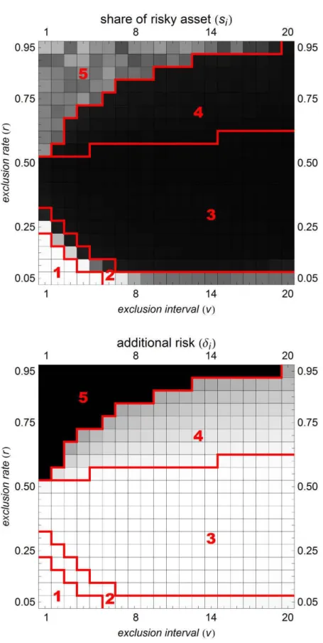
Figure 3 depicts the results of the simulation experiments in an illustrative two-dimensional scheme. The upper lattice shows the share of capital invested in the risky asset, , the bottom one the risk undertaken additionally, . Each square represents a particular setup of competition, as specified by the setting of exclusion interval v and exclusion rate r . Different gray-levels indicate the corresponding value of the dependent variables at the simulation end.

The general rule is: the darker the square, the greater the value of the respective variable. In particular, white can be read as “0”. With regard to , black stands for “1” (by definition can never exceed 1). Regarding , black stands for extremely large values. The respective squares correspond to setups in which convergence is not reached. Hence, the values would continue to rise if the simulation went on. The lattices can be divided into five numbered areas. Each area represents a characteristic asset portfolio.

-- Figure 3 about here –

Area 1: In this area, the exclusion rate r is relatively low but the exclusion interval v is short,

that is, exclusions take place relatively often. With these competitive conditions, evolution

leads to the emergence of a portfolio which consists entirely of riskless assets ( 0 ) and

does not involve any additional risk ( 0 ). As explained in Section 3.1, this configuration

belongs to the class of efficient portfolios. Related to the level of agents, the respective

- 18 -

portfolio corresponds to investors embodying maximum risk-aversion and skill, with the latter being interpreted as the ability to find an efficient composition of assets. The reason for the emergence of maximally conservative but efficient investment behavior lies in the specific requirements for survival. Due to the low exclusion rate, the prevention of extremely bad outcomes is sufficient for not being discarded. Furthermore, due to the short exclusion interval, random effects have hardly leveled out before returns are evaluated. As a result, undertaking risks is perilous, as risks raise the likelihood of attaining insufficient outcomes.

Area 2: The portfolios built in area 2 differ relative to area 1 in the parameter . Investors continue to avoid additional risk ( 0 ) but now spend a positive fraction of capital on the risky asset ( 0 1 ). Comparing the competitive conditions of area 1 and 2 reveals that this difference can be due to two reasons: a slight rise of the exclusion rate (i), or of the exclusion interval (ii). The causal paths from (i) and (ii) to the increase of are quite distinct.

By (i), the return needed to survive is enhanced. Pure risk prevention does not imply the best

probability of achieving the respective outcomes because the amount of return expectation

foregone becomes too great. Investing some capital in the risky asset increases the return

expectation and, thus, improves survivability. Accordingly, a mixture of risky and riskless

assets provides the best evolutionary fitness. By (ii), the same result is obtained through an

extension of probation time. If the exclusion interval is raised, return expectation carries more

weight because random effects tend to level out, leading to an evolutionary boost of agents

with a positive fraction of risky assets. In other words, undertaking risk becomes less perilous

for being eliminated if probation time increases. Note that the respective portfolios remain

efficient and investors still behave in a risk-averse manner, however, to a smaller degree than

in area 1.

- 19 -

Area 3: In area 3, the exclusion rate and the exclusion interval have increased further. As a result, the tendencies described above disembogue into an extreme. The fittest strategy is now simply to maximize return expectation as reflected by the fact that portfolios are composed entirely of risky assets ( 1 ). This behavior reveals that risk-prevention does not provide any competitive advantage anymore. This result can be produced by a sufficient rise of any competition parameter; r or v . If r is raised sufficiently, any sacrifice of return expectation decreases evolutionary fitness because the relatively great outcomes needed are less likely to be attained. For a sufficient rise of v , any sacrifice of return expectation is harmful because return expectation tends to become the only criterion for survival.

The investment behavior in area 3 corresponds to risk-neutrality. Risk-neutrality implies that risks are not regarded as being a “value per se”, which can be verified by the fact that agents do not undertake any risk if it does not enhance return expectation ( 0 ). Apparently, undertaking additional risk deteriorates evolutionary fitness. The reason is that the exclusion rate is still low enough so that preventing extremely bad outcomes remains paramount towards seeking extremely good ones. Additional risk, hence, is not needed but rather destructive as it raises the probability of performing badly.

Area 4: Area 4 differs from area 3 in the very inclination of agents to undertake additional risk, which now converges at some positive value ( 0 ∞ ). This behavior is risk- seeking because agents accept risks even if the latter do not contribute to the maximization of return expectation. In other words, risk is regarded as a “value per se”. The dominance of risk- seeking behavior is due to another rise of r , which has led to the transition of a critical level:

0.5 or 50%. To understand the phenomenon, assume that 1 and that the population

consists of two groups: The first group obtains a sure periodical return of μ percent. The

second group gets the same return μ but additionally plays a fair lottery which gives them a

- 20 -

50% chance for the return , respectively in case of losing. It is easy to see that for both groups, the expected periodical return (

) is equal to μ . If the population is sufficiently large, μ is also the median return; on average, half the population will achieve a return greater than μ whereas the other half falls below. However, if more than half of the population is excluded at selection periods ( 0.5 ), the median return is not sufficient to proceed. This signifies a heavy competitive disadvantage for the first group because, in contrast to the second one, they never achieve a return greater than μ . The same occurs in the simulation. By choosing 0 , agents accumulate probability mass of their return distribution near their return expectation. This is disadvantageous as the expected return does not suffice to survive. Similar agents with 0 have greater fitness as more probability mass lies above the return needed. In conclusion, risk per se generates evolutionary fitness.

Still, the explanations above do not capture all mechanisms driving the simulation results. For example, they suggest that whenever 0.5 , 0 , which, as shown by figure 3, is not true. Another fact left to clarify is the convergence of on a specific value. Let us focus the latter phenomenon first. Basically, the convergence of on

indicates that any agents with

∗

is less fit than an agent with

. The degree of risk which provides a competitive

advantage, hence, is limited. To understand the cause, reconsider the second group mentioned

above, which plays the lottery, and assume that 2 , which implies the selection criterion to

be

. Then, on average, half of the agents win in one period and lose in the other. The

resulting return

is 1 1 1 . It is easy to show that for any , this

value decreases continuously with greater | | . In other words, agents who are moderately

lucky achieve lower returns

(and thus are less likely to survive) if the variance of their

periodical returns is greater. The same happens in the model. Agents with

require

more luck than agents with

to obtain the same return

. This effect is absent if

- 21 -

1 but increases for being incremented above. As a result, agents chose lower values of , the greater . This also explains why for some 0.5 , 0 . In the model, investing in the risky asset alone can generate the optimal return variance even without undertaking additional risk.

Area 5: The results in area 5 differ sharply from all previous ones in several aspects.

Technically, the competitive conditions in this area are the only ones which do not disembogue in a convergence of portfolio parameters. In particular, the tendency of to rise does not settle down. Simultaneously, fluctuates in a range below 1; an optimal weight of risky assets does not emerge. The chaotic pattern of different gray-levels confirms that the precise value of at the simulation end is quite random. Because 1 and 0 , the portfolios built are not efficient. In contrast to all previous ones, the competitive conditions in area 5 do not provoke the predominance of agents able or willing to choose an efficient composition of assets.

The peculiarity of these results shows that the competition in area 5 follows a logic which is

very distinct. Apparently, skill is not an essential property to survive. Seeking risks, however,

becomes vitally important. Any agent improves her evolutionary fitness by raising . These

results are caused by the particular setting of competition parameters. Due to the great value

of r and relatively low v , agents require large profits in a short span of time. To increase their

chance for such profits, they need to seek risks. However, investing in an equally risky

manner than everyone else does not produce a competitive advantage. As a result, agents

force each other into taking greater and greater risks in the attempt to excel their rivals. The

counter effect described in area 4 – greater risks decreases the returns

if being

moderately lucky – is not relevant here because survival is only possible if very lucky.

- 22 -

Agents following these incentives build portfolios which enable them to attain huge profits.

The actual return of these high-risk portfolios depends largely on chance. In contrast, differences in periodical return expectation, as determined by the setting of , merely account for a minor part of actual returns. Hence, skill is of little importance. These findings mirror the insights from the theoretical analysis in chapter 2: Since the outcome needed to survive is relatively great, risk-seekers possess greater evolutionary fitness than risk-averters, even though the outcome expectation of risk-seekers is worse. As a result, the competition between agents leads to the predominance of risk-seekers who have been lucky, but who are not necessarily skilled.

Summary: The simulation results show that the fittest risk-preference is dependent significantly on competitive conditions. In this context, two competition parameters have proven to be decisive: the exclusion rate and the exclusion interval. The following relationships could be found: The greater the exclusion rate, that is, competitive pressure, the greater the advantage from risk-seeking behavior relative to risk prevention. Furthermore, the attractiveness of risky assets rises with greater exclusion interval, representing probation time, as chance tends to level out in the long run. Via these relationships, the setting of competition parameters can lead to various scenarios: risk-aversion, risk-neutrality, risk-seeking behavior and any risk preference in between can be the fittest behavior. In addition, the simulation results reflect that the more risk involved by portfolios, the more actual returns are shaped by randomness and the less by the return expectation. As a result, skill is less important for survival, the more risks agents take. This logic can lead to an extreme scenario in which competition does not select the most skilled because skill is almost entirely blurred by chance.

This scenario tends to arise if competitive pressure is intense and the great returns needed to

survive must be produced in a short span of time.

- 23 -

Of course, the above insights raise the question about the actual competitive conditions in the fund manager profession. Analyzing empirical data from 1992 to 1994, [9] finds that fear of being dismissed motivates young managers to choose low-risk portfolios. Against the background of our insights, this behavior indicates that competitive pressure was in the lower range in the time of data gathering. Future research should check if competitive conditions have changed today, which might contribute to the explanation of the attractiveness of high- risk investments.

4. C ONCLUSION

The present article explores the relationship between various competitive conditions and the evolutionary fitness of different risk preferences. The analysis is conducted theoretically as well as by an evolutionary multi-agent model that reproduces an exemplary empirical case in a stylized fashion: the competition among fund managers. This case reflects the problem very well because the risk preference of managers is a central determinant for the composition of their asset portfolio whose return managers compete about. To simulate how fund managers develop their strategies, a genetic algorithm is applied, which ensures that virtually any combination of portfolio parameters can emerge as the fittest.

On the whole, we observe that competitive environments have great influence on risk

preferences and investment behavior. Hereby, two variables play a central role. On the one

hand, there is the exclusion rate. A high exclusion rate means high competitive pressure and

creates the need for large outcomes. This makes risk-seeking behavior attractive because the

probability of high outcomes is increased. On the other hand, the time conceded to agents to

attain the outcomes is crucial as random effects tend to even out in the long-run. All in all,

these mechanisms can cause the emergence of risk-aversion in any degree but also risk-

seeking behavior.

- 24 -

The latter fact gives raise to warnings. Under competitive conditions that favor risk-seeking behavior, the importance of skill decreases because actual outcomes are determined mostly by chance. In the extreme case, survivors are not the most skilled but simply the luckiest risk- seekers. The simulation model reflects this phenomenon by showing that, in the respective competitive conditions, agents with inefficient portfolios can survive, provided that they choose high risk investments. Such scenarios are dangerous on any economic level, not only with reference to the competition between fund managers, because of two reasons. First, because the predominance of the most capable is undermined, and second, because the risky behavior of agents implies unforeseeable outcomes which run counter to economic stability.

To prevent these scenarios, our study yields two recommendations. First, competitive pressure

must be held strictly below some critical level from which risks per se generate a competitive

advantage. In the model, this is achieved by setting the exclusion rate to a low or moderate

level. Second, probation time should be sufficiently long such that skill instead of chance

shapes individual outcomes.

- 25 - References

[1] M. Allais, Le comportement de l’homme rationnel devant le risque: Critique des postulats et axiomes de l’école Américaine, Econometrica 21 (1953) 503–546.

[2] R. Amir, I.V. Evstigneev, T. Hens, K.R. Schenk-Hoppé, Market selection and survival of investment strategies, Mathematical Economics 41 (2005) 105–122.

[3] K.J. Arrow, Essays In the Theory of Risk-Bearing, Markham, Chicago, 1971.

[4] L. Blume, D. Easley, Evolution and market behavior, Journal of Economic Theory 58 (1992) 9–40.

[5] L. Blume, D. Easley, If you’re so smart, why aren’t you rich? Belief selection in complete and incomplete markets, Econometrica 74 (2006) 929–966.

[6] R.A. Brealey, S.C. Myers, Capital Investment and Valuation, McGraw-Hill, New York, 2003.

[7] W.A. Brock, C.H. Hommes, Heterogeneous beliefs and routes to chaos in a simple asset pricing model, Journal of Economic Dynamics and Control 22 (1998) 1235–1274.

[8] J. Chevalier, G. Ellison, Are some mutual fund managers better than others? Cross- sectional patterns in behavior and performance, Journal of Finance 54 (1999) 875–899.

[9] J. Chevalier, G. Ellison, Career concerns of mutual fund managers, Quarterly Journal of Economics 114 (1999) 389–432.

[10] J.B. DeLong, A. Shleifer, L.H. Summers, R.J. Waldmann, Positive feedback investment strategies and destabilizing rational speculation, Journal of Finance 45 (1990) 379–395.

[11] J.B. DeLong, A. Shleifer, L.H. Summers, R.J. Waldmann. The survival of noise traders in financial markets, Journal of Business 64 (1991) 1–19.

[12] I.V. Evstigneev, T. Hens, K.R. Schenk-Hoppé. Market selection of financial trading strategies: Global stability. Mathematical Finance 12 (2002) 329–340.

[13] M.J. Farrell, Some elementary selection processes in economics, Review of Economic Studies 37 (1970) 305–319.

[14] M. Friedman, The methodology of positive economics, in: Essays in Positive Economics, University of Chicago Press, Chicago, 1953, pp. 3–43.

[15] X. Gabaix, Power laws in economics and finance, Annual Review of Economics 1 (2009) 255–293.

[16] J.H. Golec, The Effects of mutual fund manager’s characteristics on their portfolio performance, risk and fees, Financial Services Review 5 (1996) 133–148.

[17] J.H. Holland, Adaption in Natural and Artificial Systems, University of Michigan Press,

Ann Arbor, 1975.

- 26 -

[18] C.H. Hommes, Financial markets as nonlinear adaptive evolutionary systems, Quantitative Finance 1 (2001) 149–167.

[19] D. Kahneman, A. Tversky, Prospect theory: An analysis of decision under risk.

Econometrica 47 (1979) 263–291.

[20] A. Khorana, Top management turnover: An empirical investigation of mutual fund managers, Journal of Financial Economics 40 (1996) 403–427.

[21] T. Lensberg, Investment behavior under Knightian uncertainty: An evolutionary approach, Journal of Economic Dynamics & Control 23 (1999) 1587–1604.

[22] T. Lensberg, K.R. Schenk-Hoppe, On the evolution of investment strategies and the Kelly rule: A Darwinian approach, Review of Finance 11 (2007) 25–50.

[23] M. Letteau, Explaining the facts with adaptive agents: The case of mutual fund flows, Journal of Economic Dynamics and Control 21 (1997) 1117–1147.

[24] H.M. Markowitz. Portfolio selection, Journal of Finance 7 (1952) 77–91.

[25] H.M. Markowitz. Portfolio selection: Efficient Diversification of Investments, John Wiley, New York, 1959.

[26] C. Neely, P. Weller, R. Dittmar, Is technical analysis in the foreign exchange market profitable? A genetic programming approach, Journal of Financial and Quantitative Analysis (1997) 405–426.

[27] J.-Y. Potvin, P. Soriano, M. Vallée, Generating trading rules on the stock markets with genetic programming, Computers & Operations Research 31 (2004) 1033–1047.

[28] J.B. Rosser Jr., Handbook of Research on Complexity, Edward Elgar, Cheltenham, 2009.

[29] A. Sandroni, Do markets favor agents able to make accurate predictions? Econometrica 68 (2000) 1303–1341.

[30] M.E. Schaffer, Are profit maximisers the best survivors? A Darwinian model of economic natural selection, Journal of Economic Behavior & Organization 12 (1989) 29–

45.

[31] N.N. Taleb, Fooled by Randomness, Random House, Munich, 2001.

[32] L. Tesfatsion, K. Judd, Handbook of Computational Economics: Agent-based Computational Economics, North-Holland, Amsterdam, 2006.

[33] J.W. Weibull, Evolutionary Game Theory, MIT Press, Cambridge MA, 1997.

- 27 -

Figure 1: Probability density functions of two alternative behaviors.

- 28 -

Figure 2: Risk-return diagram of portfolios possible.

- 29 -

Figure 3: Values of portfolio parameters at simulation end for variable settings of

competition parameters. Greater values indicated by darker gray tone.

- 30 - Appendix

Proof of Proposition 1:

To prove proposition 1, we have to show that the PDF of profile 2 is strictly greater than the one of profile 1 for → ∞ . Since by assumption both profiles represent normal distributions, the inequality to prove can be expressed as follows:

lim

1

√2 σ

1

√2 σ s.c.:

(i) Δ with Δ ∈ ∞; ∞

(ii) σ σ Δ with Δ 0 and σ → 0

To start, replace and by its correspondences. Logarithmize, and simplify the result. This gives:

lim

Ζ with Ζ Log σ Log σ Δ .

Next apply the equivalence setting Δ , 2σ , and

4σ Δ 2Δ . This gives:

lim

Z

Expanding in the first term and rearranging the result leads to:

lim

Δ 2Δ 2Δ

2σ Z

Expanding Z and subtracting from both sides finally yields:

Δ 2Δ 2Δ

2σ Log σ Log σ Δ

- 31 -

It can been seen that the instance of with the highest power is included in with . The limit of the left side as approaches ∞ is thus determined by the term whose limit is ∞ . Since due to (ii), the limit of the right side is greater than ∞ , the inequality is true.

q.e.d.

BERG Working Paper Series on Government and Growth

1 Mikko Puhakka and Jennifer P. Wissink , Multiple Equilibria and Coordination Failure in Cournot Competition, December 1993

2 Matthias Wrede , Steuerhinterziehung und endogenes Wachstum, December 1993 3 Mikko Puhakka , Borrowing Constraints and the Limits of Fiscal Policies, May 1994 4 Gerhard Illing , Indexierung der Staatsschuld und die Glaubwürdigkeit der Zentralbank in

einer Währungsunion, June 1994

5 Bernd Hayo , Testing Wagner`s Law for Germany from 1960 to 1993, July 1994

6 Peter Meister and Heinz-Dieter Wenzel , Budgetfinanzierung in einem föderalen System, October 1994

7 Bernd Hayo and Matthias Wrede , Fiscal Policy in a Keynesian Model of a Closed Mon- etary Union, October 1994

8 Michael Betten , Heinz-Dieter Wenzel , and Matthias Wrede , Why Income Taxation Need Not Harm Growth, October 1994

9 Heinz-Dieter Wenzel (Editor), Problems and Perspectives of the Transformation Process in Eastern Europe, August 1995

10 Gerhard Illing , Arbeitslosigkeit aus Sicht der neuen Keynesianischen Makroökonomie, September 1995

11 Matthias Wrede , Vertical and horizontal tax competition: Will uncoordinated Leviathans end up on the wrong side of the Laffer curve? December 1995

12 Heinz-Dieter Wenzel and Bernd Hayo, Are the fiscal Flows of the European Union Budget explainable by Distributional Criteria? June 1996

13 Natascha Kuhn , Finanzausgleich in Estland: Analyse der bestehenden Struktur und Überlegungen für eine Reform, June 1996

14 Heinz-Dieter Wenzel , Wirtschaftliche Entwicklungsperspektiven Turkmenistans, July 1996

15 Matthias Wrede, Öffentliche Verschuldung in einem föderalen Staat; Stabilität, vertikale Zuweisungen und Verschuldungsgrenzen, August 1996

16 Matthias Wrede , Shared Tax Sources and Public Expenditures, December 1996

17 Heinz-Dieter Wenzel and Bernd Hayo , Budget and Financial Planning in Germany, Feb- ruary 1997

18 Heinz-Dieter Wenzel , Turkmenistan: Die ökonomische Situation und Perspektiven wirt- schaftlicher Entwicklung, February 1997

19 Michael Nusser , Lohnstückkosten und internationale Wettbewerbsfähigkeit: Eine kriti- sche Würdigung, April 1997

20 Matthias Wrede , The Competition and Federalism - The Underprovision of Local Public Goods, September 1997

21 Matthias Wrede , Spillovers, Tax Competition, and Tax Earmarking, September 1997 22 Manfred Dauses , Arsène Verny , Jiri Zemánek, Allgemeine Methodik der Rechtsanglei-

chung an das EU-Recht am Beispiel der Tschechischen Republik, September 1997 23 Niklas Oldiges , Lohnt sich der Blick über den Atlantik? Neue Perspektiven für die aktu-

elle Reformdiskussion an deutschen Hochschulen, February 1998

24 Matthias Wrede, Global Environmental Problems and Actions Taken by Coalitions, May 1998

25 Alfred Maußner , Außengeld in berechenbaren Konjunkturmodellen – Modellstrukturen und numerische Eigenschaften, June 1998

26 Michael Nusser , The Implications of Innovations and Wage Structure Rigidity on Eco- nomic Growth and Unemployment: A Schumpetrian Approach to Endogenous Growth Theory, October 1998

27 Matthias Wrede , Pareto Efficiency of the Pay-as-you-go Pension System in a Three- Period-OLG Modell, December 1998

28 Michael Nusser , The Implications of Wage Structure Rigidity on Human Capital Accu- mulation, Economic Growth and Unemployment: A Schumpeterian Approach to Endog- enous Growth Theory, March 1999

29 Volker Treier, Unemployment in Reforming Countries: Causes, Fiscal Impacts and the Success of Transformation, July 1999

30 Matthias Wrede , A Note on Reliefs for Traveling Expenses to Work, July 1999

31 Andreas Billmeier , The Early Years of Inflation Targeting – Review and Outlook –, Au- gust 1999

32 Jana Kremer , Arbeitslosigkeit und Steuerpolitik, August 1999

33 Matthias Wrede , Mobility and Reliefs for Traveling Expenses to Work, September 1999 34 Heinz-Dieter Wenzel ( Herausgeber ) , Aktuelle Fragen der Finanzwissenschaft, February

2000

35 Michael Betten, Household Size and Household Utility in Intertemporal Choice, April 2000

36 Volker Treier , Steuerwettbewerb in Mittel- und Osteuropa: Eine Einschätzung anhand der Messung effektiver Grenzsteuersätze, April 2001

37 Jörg Lackenbauer und Heinz-Dieter Wenzel , Zum Stand von Transformations- und EU- Beitrittsprozess in Mittel- und Osteuropa – eine komparative Analyse, May 2001

38 Bernd Hayo und Matthias Wrede , Fiscal Equalisation: Principles and an Application to the European Union, December 2001

39 Irena Dh. Bogdani , Public Expenditure Planning in Albania, August 2002

40 Tineke Haensgen , Das Kyoto Protokoll: Eine ökonomische Analyse unter besonderer Berücksichtigung der flexiblen Mechanismen, August 2002

41 Arben Malaj and Fatmir Mema , Strategic Privatisation, its Achievements and Challeng- es, Januar 2003

42 Borbála Szüle 2003, Inside financial conglomerates, Effects in the Hungarian pension fund market, January 2003

43 Heinz-Dieter Wenzel und Stefan Hopp (Herausgeber), Seminar Volume of the Second European Doctoral Seminar (EDS), February 2003

44 Nicolas Henrik Schwarze , Ein Modell für Finanzkrisen bei Moral Hazard und Überin- vestition, April 2003

45 Holger Kächelein , Fiscal Competition on the Local Level – May commuting be a source of fiscal crises?, April 2003

46 Sibylle Wagener , Fiskalischer Föderalismus – Theoretische Grundlagen und Studie Un- garns, August 2003

47 Stefan Hopp , J.-B. Say’s 1803 Treatise and the Coordination of Economic Activity, July 2004

48 Julia Bersch , AK-Modell mit Staatsverschuldung und fixer Defizitquote, July 2004

49 Elke Thiel , European Integration of Albania: Economic Aspects, November 2004

50 Heinz-Dieter Wenzel , Jörg Lackenbauer , and Klaus J. Brösamle, Public Debt and the Future of the EU's Stability and Growth Pact, December 2004

51 Holger Kächelein , Capital Tax Competition and Partial Cooperation: Welfare Enhancing or not? December 2004

52 Kurt A. Hafner , Agglomeration, Migration and Tax Competition, January 2005

53 Felix Stübben , Jörg Lackenbauer und Heinz-Dieter Wenzel , Eine Dekade wirtschaftli- cher Transformation in den Westbalkanstaaten: Ein Überblick, November 2005

54 Arben Malaj, Fatmir Mema and Sybi Hida, Albania, Financial Management in the Edu- cation System: Higher Education, December 2005

55 Osmat Azzam , Sotiraq Dhamo and Tonin Kola, Introducing National Health Accounts in Albania, December 2005

56 Michael Teig, Fiskalische Transparenz und ökonomische Entwicklung: Der Fall Bosni- en-Hercegovina, März 2006

57 Heinz-Dieter Wenzel (Herausgeber), Der Kaspische Raum: Ausgewählte Themen zu Politik und Wirtschaft, Juli 2007

58 Tonin Kola and Elida Liko , An Empirical Assessment of Alternative Exchange Rate Regimes in Medium Term in Albania, Januar 2008

59 Felix Stübben , Europäische Energieversorgung: Status quo und Perspektiven, Juni 2008 60 Holger Kächelein, Drini Imami and Endrit Lami , A new view into Political Business

Cycles: Household Expenditures in Albania, July 2008

61 Frank Westerhoff , A simple agent-based financial market model: direct interactions and comparisons of trading profits, January 2009

62 Roberto Dieci and Frank Westerhoff , A simple model of a speculative housing market, February 2009

63 Carsten Eckel , International Trade and Retailing, April 2009

64 Björn-Christopher Witte , Temporal information gaps and market efficiency: a dynamic behavioral analysis, April 2009

65 Patrícia Miklós-Somogyi and László Balogh , The relationship between public balance

and inflation in Europe (1999-2007), June 2009

66 H.-Dieter Wenzel und Jürgen Jilke , Der Europäische Gerichtshof EuGH als Bremsklotz einer effizienten und koordinierten Unternehmensbesteuerung in Europa?, November 2009

67 György Jenei , A Post-accession Crisis? Political Developments and Public Sector Mod- ernization in Hungary, December 2009

68 Marji Lines and Frank Westerhoff , Effects of inflation expectations on macroeconomic dynamics: extrapolative versus regressive expectations, December 2009

69 Stevan Gaber , Economic Implications from Deficit Finance, January 2010

70 Abdulmenaf Bexheti, Anti-Crisis Measures in the Republic of Macedonia and their Ef- fects – Are they Sufficient?, March 2010

71 Holger Kächelein , Endrit Lami and Drini Imami, Elections Related Cycles in Publicly Supplied Goods in Albania, April 2010

72 Annamaria Pfeffer , Staatliche Zinssubvention und Auslandsverschuldung: Eine Mittel- wert-Varianz-Analyse am Beispiel Ungarn, April 2010

73 Arjan Tushaj, Market concentration in the banking sector: Evidence from Albania, April 2010

74 Pál Gervai , László Trautmann and Attila Wieszt , The mission and culture of the corpo- ration, October 2010

75 Simone Alfarano and Mishael Milaković , Identification of Interaction Effects in Survey Expectations: A Cautionary Note, October 2010

76 Johannes Kalusche , Die Auswirkungen der Steuer- und Sozialreformen der Jahre 1999- 2005 auf die automatischen Stabilisatoren Deutschlands, October 2010

77 Drini Imami, Endrit Lami and Holger Kächelein, Political cycles in income from pri- vatization – The case of Albania, January 2011

78 Reiner Franke and Frank Westerhoff, Structural Stochastic Volatility in Asset Pricing Dynamics: Estimation and Model Contest, April 2011

79 Roberto Dieci and Frank Westerhoff , On the inherent instability of international finan- cial markets: natural nonlinear interactions between stock and foreign exchange markets, April 2011

80 Christian Aßmann , Assessing the Effect of Current Account and Currency Crises on

Economic Growth, May 2011

81 Björn-Christopher Witte , Fund Managers – Why the Best Might be the Worst: On the

Evolutionary Vigor of Risk-Seeking Behavior, July 2011