Time-dependent density functional tight binding combined with the Liouville-von Neumann equation applied to AC transport
in molecular electronics
Dissertation
zur Erlangung des Doktorgrades der Naturwissenschaften (Dr. rer. nat.)
der Fakultät für Physik der Universität Regensburg
vorgelegt von Christian Oppenländer
aus
Regensburg
im Jahr 2014
Die Arbeit wurde angeleitet von: Prof. Dr. Thomas Niehaus Das Promotionsgesuch wurde eingereicht am: 07.10.2014 Das Promotionskolloquium fand statt am: 23.01.2015
Prüfungsausschuss:
Vorsitzender: Prof. Dr. Jascha Repp
1. Gutachter: Prof. Dr. Thomas Niehaus
2. Gutachter: Prof. Dr. Klaus Richter
weiterer Prüfer: Prof. Dr. Karsten Rincke
Korrekturen/Änderungen zur ursprünglich eingereichten Version:
• S. V: Inhaltsverzeichnis aktualisiert.
• S. 59: Achsenbeschriftung zur Grafik 3.17. korrigiert von "‘Gridpoint in carbon chain"’ zu "‘Grid point in Al-benzenediol-Al device"’.
• S. 79: Grafik 4.7. zeigte nicht die beschriebenen Daten und wurde ersetzt.
• S.101: Danksagungen wurden hinzugefügt.
List of publications :
[1] Christian Oppenländer, Björn Korff, Thomas Niehaus.
Higher harmonics and ac transport from time dependent density functional theory.
Journal of Computational Electronics, 12(3), 420-427. (2013)
[2] Christian Oppenländer, Björn Korff, Thomas Frauenheim, Thomas Niehaus.
Atomistic modeling of dynamical quantum transport. physica status solidi (b), 250(11), 2349-2354 (2013)
[3] Christian Lotze, Jingcheng Li, Coral Herranz-Lancho, Gunnar Schulze, Martina Corso, Setianto, Christian Oppenländer, Mario Ruben, Katharina J.
Franke, Alessandro Pecchia, Thomas A. Niehaus, Jose Ignacio Pascual.
The effect of conformational flexibility on the electrical transport through flexible molecules.
to be published.
Contents
Page
Introduction 1
1 Theoretical foundation 4
1.1 Electronic structure theory . . . 4
1.1.1 Density functional theory. . . 4
1.1.2 Density functional tight-binding . . . 9
1.2 Transport using many-body perturbation theory . . . 14
1.2.1 Green’s functions . . . 14
1.2.2 Keldysh formalism . . . 21
1.2.3 Reduced density matrix propagation . . . 24
2 Implementation 30 2.1 Ground state calculation . . . 30
2.2 Initial density matrix and time propagation . . . 33
2.3 Test calculations and examples . . . 35
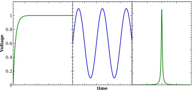
2.3.1 Typical parameters, voltage profiles and systems . . . 35
2.3.2 The outer density matrix blocks in the WBL . . . 38
3 Dynamic admittance 42 3.1 Introduction . . . 42
3.2 Connection of admittance and dc transmission . . . 43
3.3 Influence of the contacts . . . 49
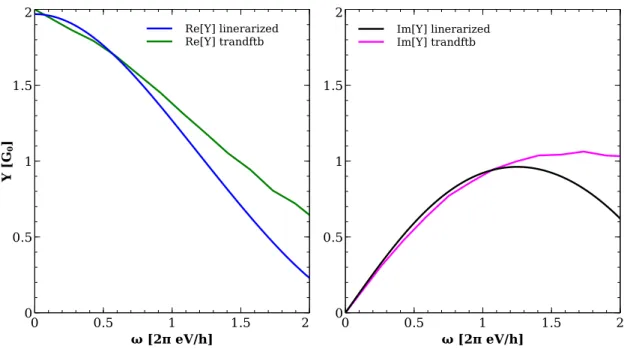
3.4 Comparison with other approaches . . . 51
3.5 Capacitance and induced charges . . . 61
3.6 Negative capacitance . . . 65
3.7 Short summary . . . 66
4 Photon-assisted tunneling and higher harmonics 68
4.1 Introduction . . . 68
4.2 Basics, Tien-Gordon approach . . . 69
4.3 PAT in symmetric junctions . . . 72
4.4 Asymmetric junctions and photocurrent . . . 80
4.5 Higher harmonics and the quasi-static current approximation . . 82
4.6 Short summary . . . 88
5 Time-independent transport through flexible adsorbed molecules 90 5.1 Introduction . . . 90
5.2 The initial geometry . . . 92
5.3 Conformational Changes during retraction . . . 94
5.4 Binding energy and forces . . . 96
5.5 Short summary . . . 97
6 Results and conclusions 99
Introduction
Molecular electronics is the bottom-up approach to the ultimate miniaturiza- tion of circuits, using individual molecules as the basic building blocks [1, 2].
While the idea itself is many decades old, only recently we have gained the experimental and theoretical capabilities necessary to do basic research in this field. Compared to silicon-based electronics, the long term goal is to provide a smaller, faster, cheaper and more flexible alternative. Even if it eventually turns out that conventional architectures cannot be efficiently replaced, a lot of valuable insight into novel quantum transport phenomena will have been gained. Today, an interdisciplinary field has emerged, combining efforts of mesoscopic physics, chemistry, material science and electrical engineering among others.
Modern molecular electronics were arguably born by the work of Aviram and Ratner [3] showing how single molecules can act as rectifiers. Due to the lack of fitting experimental techniques, a dry spell followed, which recently made way for tremendous progress: on the experimental side, the invention of the scanning tunneling microscope provided the tool to measure the conductance of single molecules. Although still a big challenge due to the large fluctuations in the acquired data, these measurements were carried out successfully, also using techniques like mechanically controlled or electrochemical break junctions. Early attempts of describing the new phenomena theoretically were succeeded by the development of the non-equilibrium Green’s function formalism. Its application to quantum transport through molecules was predominantly pioneered by Landauer, Büttiker, Meir and Wingreen. Espe- cially when combined with sophisticated electronic structure descriptions like density functional theory, the resulting ab-initio predictions are reasonably close to experiment and became today’s standard.
Within molecular electronics, time-dependent phenomena are an appealing topic due to the possibility of manipulating the current in a junction, i.e.
enhancing or decreasing the conductance by an external electromagnetic field [4, 5]. It may be possible to create optoelectronic elements like photoswitches and contacted molecules can be identified by their optical properties when emitting [6]. Below the respective plasma frequency, the laser induces an oscillating voltage of unknown amplitude in the leads and can therefore be modelled by an ac voltage under the assumption that only the leads are absorbing. This makes it possible to investigate interesting questions regarding rectification processes (also called photon-assisted tunneling), the formation of higher harmonics in the current trace or the dependence of the ac current on the incident frequency. Radiation-induced dc currents have been observed in molecular junctions by STM experiments, predominantly in the microwave regime [7], but also for optical frequencies [8], and confirmed to at least partially originate from rectification processes. For the theoretical interpretation of these experiments, the heuristic approach of Tien and Gordon is largely still in use [9], combined with a dc transmission usually calculated within density functional theory. Due to the limited accessibility, experimental data on admittance properties is much more scarce and detailed theoretical discussions are ahead of their validation.
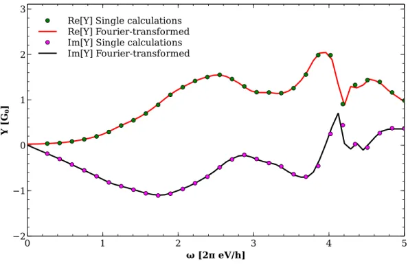
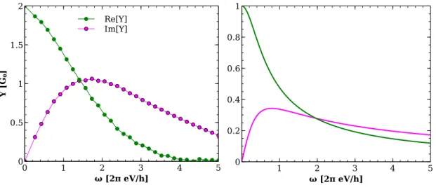
In order to describe quantum transport with harmonic oscillations in the bias theoretically, one can choose between frequency domain and time domain approaches. Using suitable approximations and for small voltages and bias amplitudes, it is possible to write down compact equations in frequency space similar to the standard time-independent Landauer formalism [10].
On the other hand, time-resolved approaches are much more flexible:
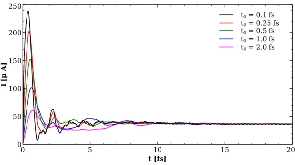
their time-dependent bias profile is not limited to harmonic oscillations, the respective amplitude can be far away from linear response, and in the case of ac transport, the frequency may be chosen in otherwise inaccessibly high regimes. Also, additional information like transients induced by switching on the bias is included. The approaches to transport may then be combined with first-principles electronic structure theory. Especially, time-dependent density functional theory (TD-DFT) has become very popular in recent years due to its efficiency that allows for realistic lead-molecule-lead systems to be calculated [11, 12, 13]. Again, there are numerous ways to describe dynamical transport using TD-DFT. One idea is to treat the whole system as a finite cluster and propagate the Kohn-Sham states through time [14, 15].
However, there are disadvantages: unphysical current oscillations persist even for large evolution times and a steady state is only transiently reached.
The approach we choose is partitioning the whole system into semi-infinite leads and a device region including layers of lead material, very similar to standard time-independent DFT-NEGF Landauer calculations. Using TD-DFT,
numerous efforts in this direction have been made before [16, 17, 18]. Since any calculation resolving the electron dynamics in a realistic system is very time-consuming, instead of DFT we use its tight-binding approximation TD- DFTB [19] to be able to calculate current traces of large systems efficiently. [20]
In Chapter 1, the necessary theoretical background will be reviewed. This in- cludes the tight-binding approximation to density functional theory, which is later combined with an equation of motion approach for the device density matrix, derived in the framework of the non-equilibrium Green’s function for- malism. In order to treat time-dependent systems, some modifications to the ground state approach have to be made, especially the solution of the Poisson equation in each time step to obtain a time-dependent potential profile. These modifications along with notes about the implementation in our code including example calculations are the topic of Chapter 2. The first of the time-dependent phenomena, the dependence of the current response amplitude on the incident frequency, is discussed in Chapter 3. Interesting questions include the informa- tion on admittance properties provided by the dc transmission, the distinction of capacitive versus inductive systems, the influence of the device potential profile and the application of the model on quantum capacitors. In Chapter 4, we investigate photon-assisted tunneling, improving on many limitations of the standard Tien-Gordon approach. The occurrence of higher harmonics and the validity of quasi-static approximations to the current response are briefly touched. Finally, Chapter 5 is reporting on a joint experimental and theoreti- cal project in which a large, flexible molecule is lifted off a copper surface and experiences characteristic jumps in its conductance.
Chapter 1
Theoretical foundation
1.1. Electronic structure theory 1.1.1. Density functional theory
Since one of the projects discussed below uses density functional theory (DFT) directly and it is also the basis of the electronic structure method we are employing in our code, this section will contain a brief review. For further details, please turn to one of the many comprehensive reviews published by the community, for example ref. [21]. and especially [22]. For DFT in the larger context of computational chemistry, see ref. [23].
Although earlier theories using density functionals exist, the main achievement lay in the two Hohenberg-Kohn theorems [24] and the Kohn-Sham equations [25] which made them a proper tool for electronic structure calculations.
Hohenberg-Kohn theorems
In many-body quantum theory, the whole information about a quantum- mechanical system is embedded in the many body wave function Ψtot(r
1, ...,rN,R
1, ...,RM), which depends on the coordinates of all the electrons riand nucleiRα. In the (usually very good) Born-Oppenheimer-approximation, one only has to solve for the electronic wave function Ψ, which is assumed to only depend on the coordinates of the electrons.
In principle, the exact Ψ for a molecule or solid could be calculated for an arbitrary non-relativistic Hamiltonian out of the time-independent Schrödinger
equation
1
X
i
−∇2i 2
−X
α
Zα
|ri−Rα|
! +
X
i<j
1
|ri−rj|
Ψ(r1, ...,rN) =EΨ(r1, ...,rN) (1.1)
where Zα is the atomic number of the respective element with core α. For a non-relativistic Coulomb-interacting system, the characterizing part is the external potential Vext =
P
ivext(ri) = −P
iα Zα
|ri−Rα|. The various possible systems only differ by this part of the Schrödinger equation if N is given.
Now, DFT states that you can use the ground-state electron density ρG(r) - which is an observable - as the system-determining quantity instead of the ex- ternal potential, and all the other ground state quantities (including Ψ) become functionals of the electronic density. This is a non-trivial suggestion since the electronic density is a function of only one vectorial variable, while Ψ de- pends on N vectorial variables. The many-body problem is formally reduced to a one-particle problem depending onρ implicitly including the information of the many-body problem. Besides its versatility, the main reason for the success of DFT stems from the fact that the transition to densities hides information which is usually not relevant, but still gives access to good approximations to quantities which are, like the total energy and as a consequence, geometries, spectra etc., resulting in an excellent ratio of practical usefulness to computa- tional cost.
The constrained search [26] algorithm is looking for the ground state wave function ΨG, which - according to the variational principle - minimizes the energy in potential vext, Evext,G, and at the same time yields the ground state electronic density ρG, which is stated as an additional condition in the mini- mization:
Evext,G = min
ΨGÏρG
hΨ|T+U+Vext|Ψi= min
ΨGÏρG
hΨ|T+U|Ψi+ Z
d3rρG(r)vext(r) (1.2) T = T[ρ] and U = U[ρ] are so-called universal functionals, since they are independent of the external potential. Due to the conceptual equality of the information included in ΨG andρG, the usual variational principle also extends to the energies calculated out of the electronic densities. This fact is usually called the second HK-theorem.
E[ρ]≥ E[ρG] (1.3)
1
Throughout this thesis, atomic units will be used.
In order to find the variational minimum of E[ρ], one needs reasonable ap- proximations to the explicit form ofT[ρ] andU[ρ], which is a highly non-trivial issue.
Kohn-Sham DFT
Kohn and Sham addressed the first challenge of finding a suitable T[ρ] [25]
and also gave the whole theory the form of single-particle equations. In the general case, the electronic density corresponds to an interacting system with a kinetic energy of Tf ull. In Kohn Sham theory, this quantity is approximated by the kinetic energyTKS which would emerge from a non-interacting system which yields the same density as the interacting one. This hypothetical non- interacting system has - apart from Koopman’s theorem [27] for exact DFT - no apparent physical meaning. In this approach, the kinetic energy is simply the sum of the kinetic energies of non-interacting particles in an effective potential specified by the interacting system to be modeled. Note that TKS becomes an implicit functional ofρ and direct minimization isn’t possible anymore.
TKS(ψ[ρ]) =−1 2
N
X
i
Z
ψi∗(r)[ρ]∇2ψi(r)[ρ]d3r (1.4)
As pointed out in [22], there are various ways to understand the approximation made here. Perhaps the most plastic one is that a wave function being a single slater determinant built out of single particle orbitals ψ[ρ] cannot represent a full many body wave function, since it ignores the effect that electrons strive to avoid each other. If the many-body wave function is a product of single particle orbitals, this simple probability superposition implies that the orbitals are independent of each other - in other words: it ignores electron correlation.
The correlation part of the kinetic energy,Tcorr =Tf ull− TKS, is put into a term called the exchange-correlation energyEXC together with all interaction effects going beyond the Hartree term UH:
UH[ρ] = 1 2
Z d3r
Z
d3r0ρ(r)ρ(r0)
|r−r0| (1.5)
EXC = (Tf ull− TKS) + (U − UH) (1.6) Every information lost by approximating exact DFT resides in approximations to this term. If it was known exactly, one could in principle calculate the full many body wave function out of the electronic density. It may be assumed that this is equally next-to-impossible as solving the Schrödinger equation itself.
However, the great advantage of DFT is that EXC is small and even rough approximations work with very good efficiency. One can also tailor the vari- ous approximations in a way suitable for the systems and quantities under study.
EXC may be decomposed in an exchange and correlation part, but as described in [23], one cannot calculate the exchange part from wave mechanic methods and use it in DFT, since its definition is different. In DFT, the definitions of ex- change and correlation are short-range only - they depend on the given point in space and the immediate vicinity around it. In wave mechanics however, both exchange and correlation have a long-range part (also called "‘static"’ correla- tion) which cancels out. Calculating exchange with wave mechanic methods and correlation with DFT, this cancellation does not longer work and leads to poor results [28].
Kohn-Sham equations
The non-interacting auxiliary system consists of single-particle equations using an effective potential:
−1 2
∇2+vKS(r)
ψi(r) =εiψi(r) (1.7) vKS =vext+vH+vXC (1.8) where vext is the potential one would like to solve the many-body system for, vH is the Hartree potential and vXC =
δEXC[ρ]
δρ . Note that the symbol δ means a functional derivative. The density solving this set of single-particle Schrödinger equations is equal to the density minimizing the energy functional, thus all that is left to be done is solving these Kohn-Sham equations. Since the electronic density is calculated from the occupied orbitals (the lowest N spin-eigenfunctions are filled),
ρ(r) =
occ
X
i
|ψi(r)|2 (1.9)
while the effective potential and thus the orbitals are modified by the electronic density via:
δ(Vext[ρ] +UH[ρ] +EXC[ρ])
δρ =vKS(r) (1.10)
These equations have to be solved self-consistently. Once convergence has been reached, all relevant observables can be calculated from the obtained
approximate ground state electronic density. With EKS =TKS+
R d3rvKS(r) = PN
i εi (note that the total energy of the KS-system is not the total energy of the interacting system), one can easily derive a good-to-handle formula for the ground state energy EG:
EG =
N
X
i
εi−1 2
Z Z
d3rd3r0ρG(r)ρG(r0)
|r−r0|
| {z }
UH[ρG]
− Z
d3rvXC(r)ρG(r) +EXC[ρG] (1.11)
General DFT performance and used XC functionals
One of the main reasons DFT performs very well even for quantities which scale at tiny fractions of the total energy (like cohesive energies) is that most of the error the standard XC functionals make is systematic and benefits from error correction. One has to be careful comparing properties in reactions involving phase transitions or other significant system changes, though. Ob- viously, since DFT is formally exact, the key quantity for the accuracy - apart from numerical limitations - is the XC functional one decides to use.
Local density approximation
The LDA is a very crude, simple approximation and still works surprisingly well. It assumes that the density varies slowly and the resulting exchange energy EXLDA can be described as the one of an uniform electron gas [26] [29]:
EXLDA[ρ] =−const· Z
d3rρ(r)
4
3 (1.12)
The correlation part ECLDA of the LDA is added from quantum monte carlo simulations, and the available methods [30] [31] yield very similar results. It systematically (!) underestimates EX by about 10% [23], yet overestimates EC, and therefore benefits from error correction in most systems.
Important for later discussions is the characteristic of LDA to overbind molecules and solids. Binding energies are generally too large, leading to lattice constants and molecular binding distances about 1-3 % too small. But since these deviations are systematic, comparisons between similar systems can still be very good. Since LDA is local, it fails to describe Van-der-Waals interactions which leads to error correction with the general overbinding.
Generalized gradient approximations
As mentioned, LDA takes the density to be constant in the vicinity of the space point it is evaluated at. GGAs include information about the change in density close to the evaluation point. These functionals are often called semi-local, but since they mathematically only depend on one space-point, it makes more sense to also call them local. The general form of these functionals is:
EXCGGA[ρ] = Z
d3rf(ρ(r), ∇ρ(r)) (1.13)
While it could be stated there is only ”one“ LDA, this is entirely untrue for GGAs. They differ in the amount of empirical parameters, assumptions and their entire functional form within the general concept. GGAs yield binding energies closer to the experimental results, but their error is less systematic: although they usually under-bind, they can also overbind. This leads to problems when comparing systems in which the functional behaves differently. In our code for time-dependent calculations, we choose to build our DFTB Hamiltonian using the GGA functional PBE [32] for its overall good performance.
1.1.2. Density functional tight-binding
Although DFT is fast compared to wave function methods, the quantum me- chanical treatment of larger systems is still a tedious business, and especially time-dependent approaches can become very expensive. There is room for another (reasonable) approximation, and despite its crude appearance, DFTB is a sophisticated approach towards a quantum mechanical description narrowing the gap in computational cost between DFT and force field methods.
Tight-binding
Tight-binding approaches became common due to Slater and Koster in 1954 [33] who approximated the full LCAO (linear combination of atomic orbitals) method for solids. The exact many-body Hamiltonian is approximated by parametrized matrix elements. The wave function is expanded into atomic-like orbitalsφν located at center αwhich are not necessarily solutions to the atomic problem, but share the same symmetries. Since they are non-orthogonal in the general case, they have to be transformed to an orthogonal basis by a Löwdin
transformation using their overlap matrix S: ψαν =
X
α0ν0
Sαα−1/20νν0φα0ν0 (1.14)
For a solid, the Hamiltonian is now written in Bloch sums over the atomic orbitals as
Hνα,µβ = X
Rβ
eik(Rβ−Rα) Z
drψνα∗ (r−Rα)Hψµβ(r−Rβ) (1.15)
The various different tight-binding models have in common that the integral in the above equation is replaced by a parameter which only depends on the distance |Rα−Rβ| between two centers and the symmetry of the respective orbitals [34]. The first assumption implies the two center approximation, which states that all matrix elements connecting three or more centers are neglected.
If the method is to be used on a finite system, a total energy expression is needed. In addition to the bandstructure termEBS, a repulsive energy resulting from a sum of pair terms is used to approximate the terms not included in the bandstructure energy, yielding a tight-binding total energy ETB as [35].
ETB =
N
X
i=1
εi
| {z }
EBS
+ 1 2
X
α
X
α6=β
Erep(|Rα−Rβ|) (1.16)
where the first term is the sum of the occupied single electron energy eigenvalues of the above Hamiltonian and the second term is the repulsive correction which also depends only on the distance between two centers.
All terms which do not fit in this form are neglected. Most tight-binding approaches and especially the classical ones are semi-empirical, they use a set of parameters given by experiment to build up the necessary terms for calculating the total energy, leading to limited transferability. However, the scheme is very fast since there are few things to calculate at runtime.
DFTB
The idea is now to find transferable parameter sets from DFT with ab-initio functionals, making the whole TB-approach completely free of experimental data, while keeping the advantage of in this case pre-calculated look-up tables
to considerably speed up the calculations.
It is not straightforward why casting DFT into the tight-binding form and drop- ping all self-consistency should be a reasonable approximation, for a justifica- tion see [36]. In short, DFTB can be seen as a stationary approximation to DFT.
At the core of DFTB is an expansion of the total energy expression around a reference density ρ0, which takes the following form [36] [37]:
EDF TB =
occ
X
i
hψi|H
0|ψii − 1 2
Z Z 0
d3rd3r0 ρ0
0ρ0
|r−r0|+EXC[ρ
0]− Z
d3rvXC[ρ
0]ρ
0
(1.17) +
1 2
M
X
α,β
ZαZβ
|Rα−Rβ|+ 1 2
Z Z 0 1
|r−r0| +
δ2EXC δρδρ0 ρ
0
δρδρ0... (1.18)
where H0 is a non-self-consistent DFT Hamiltonian evaluated at the reference density. The last term is the second order contribution and constitutes second order DFTB or self consistent charge (SCC) DFTB. Even without this term, the method performs quite well - however, in order to describe systems with large charge transfers, one has to self-consistently reposition the partial charges using this second order term [37]. For now, we concentrate on the zeroth order (there are no linear terms).
Applying the LCAO method on DFT, ψi(r) =
X
ν
Cνiφν(r−Rα) (1.19)
one has to solve the set of single particle Kohn Sham equations X
ν
Cνi(hφµ|H|φνi
| {z }
Hµν
−εihφµ|φνi
| {z }
Sµν
) = 0 (1.20)
with the mentioned (two-center) approximations to the Hamiltonian matrix, defining an effective potential Vef f(r) =Vext(r) +VH[ρ(r)] +VXCLDA[ρ(r)]:
Hµν=
εµAtom if µ=ν
hφµ|T+Vef f[ρα
0 +ρβ
0]|φνi if µ ∈ α, ν ∈ β
0 otherwise
(1.21)
In the two-center term, one can either choose a density superposition (Vef f[ρα
0 +ρβ
0]) or a potential superposition (Vef f[ρα
0] +Vef f[ρβ
0]). In the case of our calculations, a density superposition is chosen.
If the expansion around ρ
0 is to be accurate, it has to be a good approxima- tion to the density DFT calculations would yield. Therefore, ρ
0 is assumed to be a superposition of compressed atomic densities calculated within DFT. In molecules and solids, the electrons have less space to move, and therefore a compression term adds to a better description of the superposed densities.
Furthermore, the atomic DFT calculations yield wavefunctions that can be used as a minimal set of basis functions which perform very well, since they in turn consist of multiple basis functions. The modified single-electron Kohn-Sham equations to calculate the pseudo-atomic orbitals read [19]:
"
T+Vef f(r) + r
r0 2
#
φν(r) =ενpsatφν(r) (1.22)
with a compression radius r
0. The atomic-like orbitals are hereby written in terms of Slater-type orbitals (STOs) and spherical harmonics Ωlm as [19]
φν(r) = X
n,β,lν,mν
rlν+ne−βrΩlνmν
r r
(1.23)
with the quantum numbers n, l, m and β being a parameter of which five different values have been shown to be a sufficient description for elements within the first three rows. [38]
Once the band structure energy has been calculated, the repulsive part can be fitted with a spline to self-consistent DFT calculations. The reference system used for the fit depends on the systems one would like to calculate with the DFTB approach. Generally, one can use diatomic molecules as a reference, but the closer the reference system of the fit is to the properties of the system DFTB is used for, the more accurate the repulsive part of the total energy will be. However, one can in principle access the full information contained in the self-consistent calculation.
Erep(|Rα−Rβ|) = (EDF T− EBS)|
reference system (1.24)
Together with the spline, the Hamiltonian and Overlap (Sµν) matrices are stored for finite step sizes in the interatomic distance. Implementations of DFTB look up these tables - called Slater Koster (SK) files - and can
immediately write down and diagonalize the matrices out of information about the system geometry.
SCC-DFTB
SCC-DFTB takes the next step towards a better description - especially of highly inhomogeneous systems - but reintroduces the need of a self-consistent cycle at runtime. The key arguments of Elstner et al. [37] will be restated here.
First, one divides the density fluctuations into atom-centered partsδρα and δρβ, writes down a multipole expansion into radial (Fml) and angular (Ωlm) parts, cutting after the monopole term:
δρα(r) = X
l,m
KmlFmlα (|r−Rα|)Ωlm
r−Rα
|r−Rα|
(1.25)
≈∆qαFα
00(|r−Rα|)Ω00 (1.26)
Here, ∆qα is the net charge on the respective atom and Fα
00 the normalized spherical density fluctuation. Inserting this expansion into the 2nd order term yields the following form:
E2nd = 1 2
N
X
α,β
∆qα∆qβγαβ (1.27)
γαβ contains all quantities of the expansions excluding the net charges ∆qα,β. According to [39], the on-site terms γαα can be approximated by the difference between the atomic ionization potentialIα and electron affinity Aα of the atom centered atα, which again can be well approximated by the so-called Hubbard parameter Uα. This quantity can be calculated within DFT as follows:
Uα =
∂2Eα
∂n2HOAO ≈ Iα− Aα (1.28)
wherenHOAO is the occupation number of the highest occupied atomic orbital and Eα the total energy of the neutral atom at α. In the limit of large dis- tances, γαβ shows a
1
|Rα−Rβ| behavior, the interaction is thus decaying into a purely Coulomb-like one with vanishing XC contributions. Ref. [37] describes the derivation of an analytical expression for γαβ with the correct long range
behavior. The authors assume an exponential decay of the density and deter- mine the decay constant through the Hubbard parameters. The total energy expression now reads to second order of DFTB:
E2nd(Uα, Uβ, |Rα− Rβ|) =
occ
X
i
hφi|H0|φii+ 1 2
N
X
α,β
γαβ∆qα∆qβ+Erep (1.29)
In order to get the net charges ∆q, one calculates the Mulliken charges as an approximation to the atomic charge and subtracts the charge of the neutral atom.
∆qα = 1 2
occ
X
i
ni
X
µ∈α N
X
ν
(Cµi∗ CνiSµν+C∗νiCµiSνµ)− qα0 (1.30)
with Cµi, Cνi being the expansion coefficients of the LCAO. The Kohn-Sham equations look the same as before, with an additional term in the Hamiltonian matrix.
Hµν =hφµ|H
0|φνi+ 1 2
Sµν
N
X
ξ
(γαξ +γβξ)∆qξ (1.31)
1.2. Transport using many-body perturbation theory 1.2.1. Green’s functions
The goal of this section is to review the non-equilibrium Green’s function (NEGF) formalism [40, 41] which is able to tackle a variety of even time- dependent transport scenarios. These include also interacting electrons in the device region (not within the leads) to all orders of perturbation theory and far away from equilibrium. The application of this NEGF (or Keldysh) formalism to static transport using a mean-field approximation like in the Landauer [42,43]
context is only a small part of what it is capable of and does not use its full potential. However, a combination of NEGF with DFT became a very popular approach also to static time-independent transport [44, 45] as explained below.
Please note that in the whole theoretical introduction, we assume the overlap matrix Sµν = hφµ|φνi of the atomic orbitals to be equal to the identity matrix for simplicity. The results must therefore be straightforwardly generalized to fit to the non-orthogonal basis sets in use by our DFTB implementation. The first part of this introduction roughly follows Ref. [46].
Basics
One first needs to introduce the simplest kind of Green’s Functions for non- interacting single particles. In the mathematical sense, a Green’s Function is a way to solve a linear differential equation and its usefulness is therefore not limited to the Schrödinger equation. However, in its context, the Green’s Function operatorG solves
i d
dt − H
Gr/a(t) =1δ(t) (1.32)
where 1 is the identity matrix and the r/a subscript indicates two solutions:
The retarded Green’s Function Gr(t − t0) propagates the state vector forward in time from t
0 to t. It includes information about the history of the entire system. Its counterpart, the advanced Green’s Function Ga(t − t
0), propagates the state backwards in time from t0 to a t with t < t0. It includes information about the future state of a system.
Formally, the solutions to the equations of motion for these Green’s Functions look very much alike the time propagation operator for a time-independent Hamiltonian:
Gr(t − t
0) =
−ie−iH(t−t0) t > t
0
0 t < t
0
(1.33) Ga(t − t
0) =
0 t > t0 +ie−iH(t−t0) t < t
0
(1.34) (1.35) Both solutions are connected via
[Gr(t)]
†
=Ga(−t) (1.36)
In the following, Gr/a(t) will refer to the Green’s Functions defined by a Schrödinger equation with the full Hamiltonian of a system consisting of the kinetic term and a scattering potential V(r):
Htot =−1 2
∇2+V(r) (1.37)
whereasGr/a
0 (t) are solutions to the "‘free"’ Hamiltonian without any scattering potential. Note that this kind of Green’s Functions does only depend on the
time difference (t − t
0) and it is therefore possible to Fourier transform them into energy space. However, in order to converge the integration, one has to add an exponential term e±ηt with an infinitesimal η >0 as shown below. The sign in front of this parameter is also the distinction between retarded and advanced Green’s Functions in energy space.
Gr(E) = Z +∞
−∞
dt eiEte−ηtGr(t) (1.38)
One then easily obtains
Gr(E) = [E1− H+iη]
−1
(1.39) Ga(E) = [E1− H − iη]
−1
(1.40) (1.41) showing that these functions have poles at the energy eigenvalues of the re- spective Hamiltonian.
Self-Energy and the Dyson equation
In general, the self-energy Σ describes the effects of an interaction with its environment on the energy of a single particle. Treating the interactions as a perturbation series, one can visualize them as Feynman diagrams as known from quantum field theory. What exactly the self-energy is describing depends on what is defined as the environment. It could only include the effects of leads on a nanodevice with non-interacting electrons like in the Landauer approach, or it could additionally include the effects of electron-electron and/or electron-phonon interactions on the single particles subjected to them.
If the perturbative series is converging, there is a finite self-energy one can - in principle - calculate and modify the single particle energies so they contain all the respective interactions.
In the context of Green’s Functions, one can easily calculate Gr/a
0 for an un- perturbed Hamiltonian, but needs Gr/a for the description of the system. The relation between the two depends on the interactions added by the perturbation and thus on the self-energy. The important Dyson equation
2
is stating exactly this:
2
Which equations are called "Dyson equation" is not uniform in the literature. The true, most general Dyson equation looks very similar to the equation given here but contains operators defined by many-body perturbation theory, unlike the simple Green’s Functions in this section.
It is able to describe interacting systems out of equilibrium as stated in the NEGF sections.
Gr/a(t − t
0) =Gr/a
0 (t − t
0) + Z t
t0
dt0 Z t0
t0
dt00Gr/a
0 (t − t0)Σ
r/a
(t0− t00)Gr/a(t00− t
0) (1.42)
=Gr/a
0 (t − t0) + Z t
t0
dt0 Z t0
t0
dt00Gr/a(t − t0)Σ
r/a
(t0− t00)Gr/a
0 (t00− t0) (1.43) The integration sums up interactions for an ingoing propagator at t
0 which is affected by interactions at the intermediate times and becomes the outgoing propagator at time t. One can extract the orders of the perturbation by attempting an iterative solution: set Gr/a = Gr/a
0 (Born approximation) and keep re-inserting the so-calculated approximative full Green’s Function into the Dyson equation. This way the equation is transformed into an infinite series.
In the case of the mean-field approximation employed in the Landauer formal- ism, the self-energy is simply the scattering potential:
Σ(t0− t00) =V δ(t0− t00) (1.44) and the Dyson equation reduces to the Lippmann-Schwinger equation in the scattering context:
Gr/a(t − t
0) =Gr/a
0 (t − t
0) + Z t
t0
dt0Gr/a
0 (t − t0)V Gr/a(t0− t
0) (1.45)
=Gr/a
0 (t − t
0) + Z t
t0
dt0Gr/a(t − t0)V Gr/a
0 (t0− t
0) (1.46) Generally, if the Green’s functions only depend on time differences, the Dyson equation can be transformed into energy space, where it looks more conve- nient.
Gr/a(E) =Gr/a
0 (E) +Gr/a(E)Σ
r/a
(E)Gr/a
0 (E) (1.47)
More importantly, there is an alternative form of the Dyson equation often encountered,
Gr/a(E) =
E1− H −Σ
r/a
(E)∓ iη−1
(1.48) which nicely shows how the self-energy affects (renormalizes) the single- particle energies at the poles of the Green’s function defined by the Hamiltonian
eigenvalues. The real part adds a shift to the energy levels and the imaginary part adds a lifetime for these states to which it is inversely proportional. In the above case of a full unpartitioned mean-field system Hamiltonian, the imaginary part of the self-energy is zero and consequently, the lifetime of the states is infinite. The real part here adds a rigid shift which is not energy dependent.
However, it is important to realize here that this shape of the self-energy only applies to a scattering system which is described as a whole by a full Hamiltonian and not partitioned into leads and device region. For all practical purposes we only want to describe a device region artificially coupled to semi- infinite leads, as described in the next section. In this case, the self-energy looks different even in a Landauer scattering approach using the mean-field approximation, since now it describes the effect of the interaction with the leads on the energies of single electrons within the device only.
Standard partitioning
As mentioned in the last section, the two-probe systems we would like to in- vestigate are usually partitioned into a device region (D) and two semi-infinite leads, left (L) and right (R). The device region itself consists of a molecule or an atomic chain which will be called inner device (ID) and a few layers of lead material (see Fig. 1.1). Adding lead material provides screening at the in- terfaces and a smoother potential transition to the semi-infinite leads that are assumed to be uniform. The coupling between leads and device is mediated by short-ranged off-diagonal blocks of the system Hamiltonian, TLD and TRD.
Figure 1.1: Schematic of the setup. The device region is connected to the left and right semi-infinite lead by open boundary conditions. The device contains lead material, the current is measured at the interfaces SL, SR.
The Hamiltonian may then be partitioned (in matrix notation) as
HL TLD 0 TLD† HD TRD†
0 TRD HR
|φLi
|φDi
|φRi
=E
|φLi
|φDi
|φRi
(1.49)
and inserting the Green’s Functions of the lead regions as GL,Rr/a =
E1− HL,R± iη−1
(1.50) leaves us, after solving the system of equations, with an expression for |φDi:
[E1− HD− TLD† GLr/a(E)TLD
| {z }
Σ
r/a L (E)
− TLR† GRr/a(E)TRD
| {z }
Σ
r/a R (E)
]|φDi= 0 (1.51)
Comparing with the definition of the non-interacting single-particle Green’s function and the alternative form of the Dyson equation leads to an identifica- tion of the self energy terms as shown in the curly brackets above.
Gr/a(E) =
E1− HD−Σ
r/a
L (E)−Σ
r/a R (E)
−1
(1.52) Please note the difference between the Green’s function of the isolated device region GCr/a and the Green’s function of the device region in the presence of the leads Gr/a, the one we are looking for.
So, in order to obtain Gr/a, we need the coupling terms of the Hamilto- nian and the Green’s functions of the leads. Since the leads are assumed semi-infinite, this is not straightforward. However, there are methods to calculate a so-called surface Green’s function which uses the periodicity of the leads to obtain a finite function. It can then be used to calculate the self-energy and thus the device Green’s function which contains all the information about the transport properties. Along the transport direction, the leads are divided up in identical principal layers which only interact with their nearest neighbor layer. Since there is also one principal layer of lead material in the device region, the coupling block between device and lead is restricted to one lead principal layer and almost identical to the repeating coupling between two lead layers. Therefore, only the surface block of the lead Green’s functions is needed to obtain the self-energy. How exactly the surface Green’s functions are being calculated will be explained in section 3.2.2.
For now, let us review the consequences of the system partitioning on the shape of the self-energy and the implications of that. The real part of Σ
r/a L/R and therefore the energy shift is generally energy-dependent. More importantly, the self energy will acquire an imaginary part adding a finite lifetime to the states in the device, describing a scattering from the device into the leads. We define the energy-dependent scattering rates
ΓL,R(E) =−2Im{Σ
r
L,R(E)} (1.53)
This is equivalent to a broadening of the level in energy space, which is why the Γ = ΓR+ ΓR will frequently be called linewidth or broadening (matrix).
Note that the partitioning does not add any new physics at all, and the different shape of the self-energy is only due to the fact that we are looking at a part of the system only. Of course, the same energy level shift and broadening would also be there if one looks at the full unpartitioned Hamiltonian - but it would be well hidden in a massive Green’s function for the whole system and not be describable by self-energies.
Landauer transmission using Green’s functions
At this point it is possible to derive an explicit Landauer transmission using the Green’s functions we introduced. In the literature, this expression is frequently derived employing the NEGF formalism, but employing the same approxima- tions as the derivation via the scattering approach. Especially this means that we are looking at a time-independent steady state, interactions are only treated at mean-field level and we have no electron-electron interactions explicitly in- cluded. An equation for the current I through the the junction from left to right of the form
I = 1 π
Z +∞
−∞
dE [fL(E)− fR(E)]T(E) (1.54)
is called "‘Landauer formula"’ when the transmission function T(E) can be written in this simple form only dependent on energy. fL and fR denote the Fermi functions of the respective lead subjected to a voltage V. At zero temperature, they are equal to one at EF ± eV
2 , respectively, and equal to zero above the respective energies, defining a bias window. The NEGF formalism is able to additionally derive an equation that also describes a scattering approach, but with interacting electrons in the device region (not in the leads though). The resulting equation is often referred to as Meir-Wingreen
formula or extended Landauer formula [47].
Without introducing NEGF and employing many-body perturbation theory, it is still possible to derive the following Landauer-type expression by the use of the Fisher-Lee-relations [48] which create a connection between the Green’s functions and the scattering matrix of the usual wave-function-based scattering approach.
I = 1 π
Z +∞
−∞
dE[fL(E)− fR(E)] Tr[ΓRGrΓLGa] (1.55)
Comparison with1.54identifies the transmission function. The current is deter- mined by the trace over a matrix with the dimension of the number of orbitals in the device region. Using NEGF in the time-independent non-interacting limit will yield the same expression. It is the main equation for static single-electron Landauer transport.
1.2.2. Keldysh formalism
Preparation: equilibrium
In order to use Green’s functions to go beyond static non-interacting trans- port, one has to employ many-body perturbation techniques. The resulting propagators are not simply a solution to a linear differential equation as the functions introduced before, but are nevertheless called by the same name.
Specifically, they may contain averages over four or more field operators and there exists no corresponding closed differential equation that the respective Green’s function can solve [49]. One should therefore view many-body Green’s functions as a different object which still share many of the features of their non-interacting single-particle version.
NEGF is exact for time-dependent closed systems (which may have open boundary conditions, but they must not be "open" in the sense that Hamiltonian dynamics are not valid anymore) and far away of equilibrium. It uses all orders of perturbation theory, but obviously the description breaks down once used in cases where many-body perturbation theory isn’t applicable at all, like the Kondo effect. Since the Keldysh formalism is a natural extension to equilibrium many body techniques, the latter are introduced here before- hand. The following review will be based on the book by Cuevas and Scheer [1].
The time-evolution operator in the interaction picture as a perturbation expan-